Application of a Model that Combines the YOLOv3 Object Detection Algorithm and Canny Edge Detection Algorithm to Detect Highway Accidents

Abstract

This study proposed a model for highway accident detection that combines the You Only Look Once v3 (YOLOv3) object detection algorithm and Canny edge detection algorithm. It not only detects whether an accident has occurred in front of a vehicle, but further performs a preliminary classification of the accident to determine its severity. First, this study established a dataset consisting of around 4500 images mainly taken from the angle of view of dashcams from an open-source online platform. The dataset was named the Highway Dashcam Car Accident for Classification System (HDCA-CS) and was developed with the aim of conforming to the setting of this study. The HDCA-CS not only considers weather conditions (rainy days, foggy days, nighttime settings, and other low-visibility conditions), but also various types of accidents, thus increasing the diversity of the dataset. In addition, we proposed two types of accidents—accidents involving damaged cars and accidents involving overturned cars—and developed three different design methods for comparing vehicles involved in accidents involving damaged cars. Canny edge detection algorithm processed single high-resolution images of accidents were also added to compensate for the low volume of accident data, thereby addressing the problem of data imbalance for training purposes. Lastly, the results showed that the proposed model achieved a mean average precision (mAP) of 62.60% when applied to the HDCA-CS testing dataset. When comparing the proposed model with a benchmark model, two abovementioned accident types were combined to allow the proposed model to produce binary classification outputs (i.e., non-occurrence and occurrence of an accident). The HDCA-CS was then applied to the two models, and testing was conducted using single high-resolution images. At 76.42%, the mAP of the proposed model outperformed the benchmark model’s 75.18%; and if we were to apply the proposed model to only test scenarios in which an accident has occurred, its performance would be even better relative to the benchmark. Therefore, our findings demonstrate that our proposed model is superior to other existing models.

1. Introduction

1.1. Background

The rapidly developing technology of deep learning has been widely applied in recent years. As a novel field of study, deep learning seeks to analyze and interpret data by mimicking and simulating the way in which the human brain operates. The core aspect of deep learning is to train multilayer neural network models using large volumes of data to determine input-output relationships. The number of layers in a model, the number of neurons in each layer, how the neurons are connected, and how the functions are simulated and determined based on the problem at hand. The weights and biases of each layer are updated using large volumes of data. Deep learning has been extensively applied and has contributed to the development of image recognition and object detection technologies, which utilize convolutional neural networks (CNNs) as a basis for extracting the features of an image [1]. The objective of image recognition is to acquire information from an image (the information of the object with the most prominent features); the objective of object detection is to acquire more information from multiple objects in an image, such as acquiring the precise position and attributes of each target object in an image. While the history of object detection dates back 20 years, major breakthroughs were only achieved in 2014, during which enhancements in the computational capability of a graphics processing unit (GPU), as well as advancements in deep learning-based image recognition techniques, were attained. For this reason, the year 2014 is considered a watershed moment in the field of object detection, marking the shift from traditional methods to deep learning-based methods. 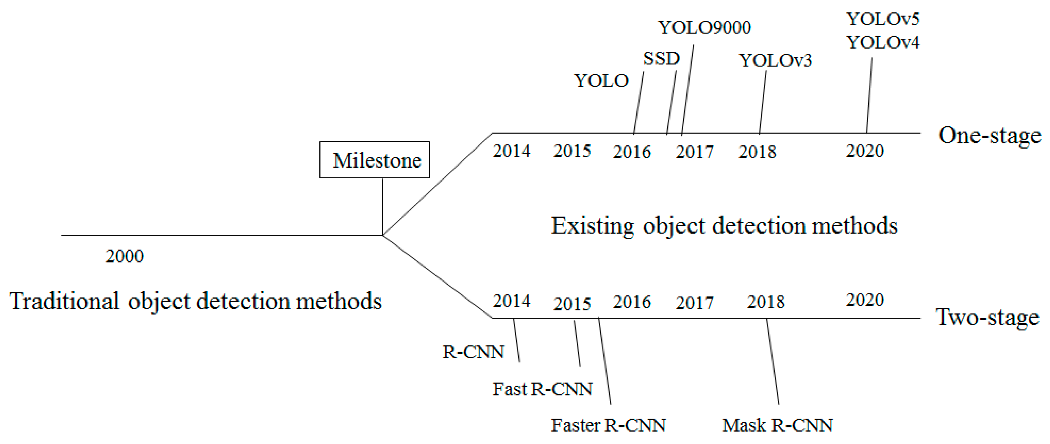Figure 1 depicts the developmental history of object detection algorithms.

There have been notable developments in object detection techniques. A two-stage approach-based Region-CNN (R-CNN) [2], which was developed in 2014 and works by separating an image into different regions of interest, is representative of these developments. Subsequently, Fast R-CNN [3] and Faster R-CNN [4] were developed following optimizations made to R-CNN, which enhanced the accuracy and speed of detection. Most recently, the development of Mask R-CNN [5] is considered revolutionary as it not only detects the position and type of a target object, but also extends into the field of semantic segmentation, which means that Mask R-CNN is able to illustrate the contours of a target position. The aforementioned algorithm models separate an image into many regions during detection and are characterized by higher accuracy, but longer computational times, which hinder their use in real-time applications. Therefore, one-stage approach models based on regression algorithms have been proposed. These models perform regression analyses of targets of detection and directly predict the locations of the targets. While it offers faster compute speeds, this method has a lower accuracy relative to the aforementioned methods as it utilizes single-shot detection to process an image. Nevertheless, it is able to perform real-time calculations, while maintaining accuracy within an acceptable range, making it less time-consuming. Representative one-stage object detection models include Single-Shot Detectors (SSD) [6] and the You Only Look Once (YOLO) series (such as YOLO [7], YOLO9000 [8], YOLOv3 [9], YOLOv4 [10], YOLOv5 [11]). The development of these models can help address the need for real-time object recognition. The newly released YOLOv4 and YOLOv5 have a detection speed that exceeds that of the two-stage approach and is more accurate than many two-stage and one-stage approaches. Even though YOLOv4 or YOLOv5 should have been used in this study by virtue of its real-time capabilities and better accuracy, we also had to consider that fact that this study was focused on practical applications, and that the YOLOv4 and YOLOv5 were only launched at the end of April 2020 and at the early of June 2020, respectively, and have yet to be subjected to extensive and robust testing. Despite the model’s significant improvements in accuracy and real-time capabilities, we also had to take into account that an accident detection method should be stable and well-developed. Moreover, the complex network structure of YOLOv4 and YOLOv5 requires higher computational volumes, and consequently, relies on high-level (and costlier) graphics cards, such as the RTX 2080Ti, to attain a better learning performance. With suitability for the practical application being a primary consideration, YOLOv3 was chosen as the object detection algorithm for this study as it offered better operational timeliness, detection accuracy, and stability, while also being better suited for use with cheaper mid-to-high-end GPUs, i.e., even though YOLOv4 or YOLOv5 is newer and more advanced, its performance requirements are also higher and cheaper GPUs are not as capable of handling it.

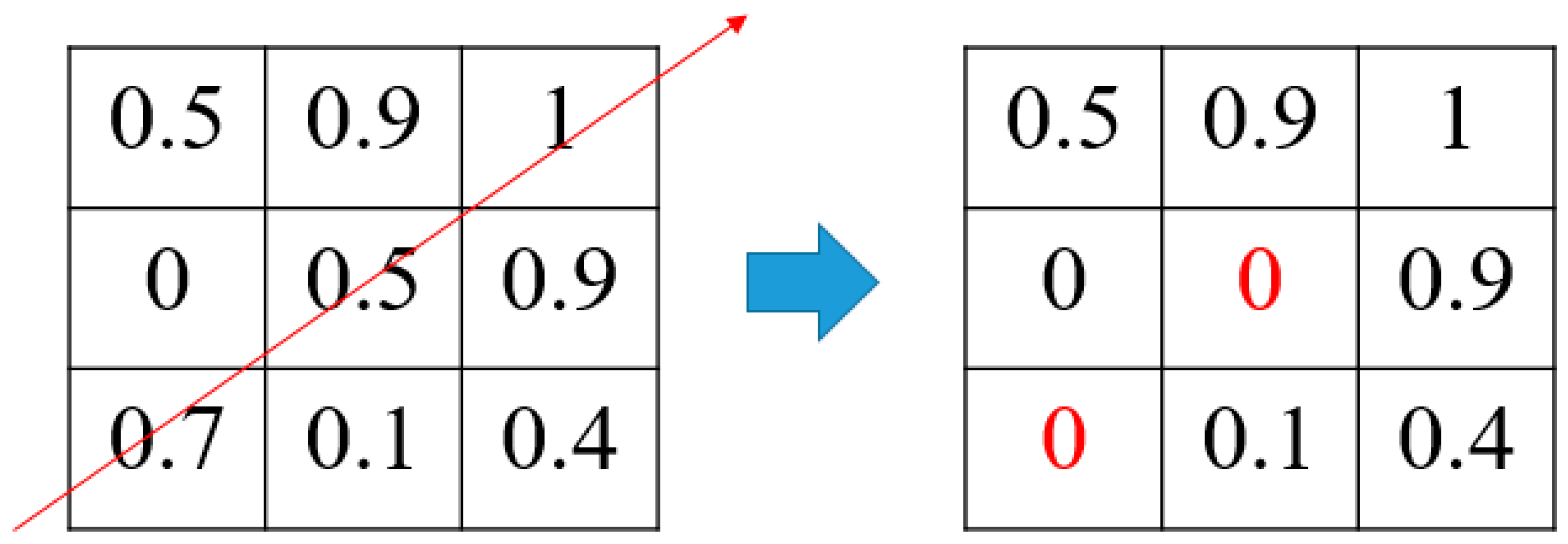
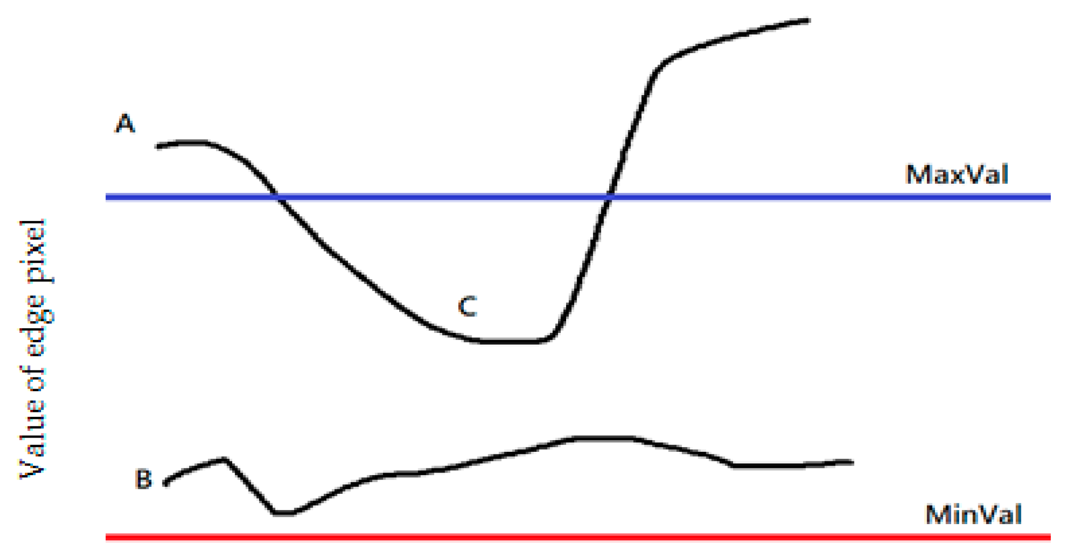
Meanwhile, image processing plays a salient role in object detection technology. Its function is to help acquire a higher volume of more usable information, in addition to achieving more reliable detections, analyses, learning outcomes, and applications. A color image consists of three superimposing layers of red, blue, and green (RGB) images, and is formed by different pixels with distinct positions and grayscale values. Images are often filtered to achieve noise removal and image enhancement. Furthermore, image segmentation is an important step in image processing. In image segmentation, an image is partitioned into different components or objects. Thresholding is the most common form of image processing and involves turning the pixels of an image into binary values. Specifically, pixels with pixel values that do not attain a threshold value are defined as 0 (all-black), while pixels with pixel values that are equal to or exceed the threshold value are defined as 1 (all-white). The most common application of thresholding is edge detection, such as the Canny edge detection algorithm [12]. The advantage of image processing is the salient role it plays in smart vehicles, especially at night, when the low visibility and brightness result in grainy images. Therefore, adjusting the brightness and contrast or enhancing the details during image processing can increase driver safety.

1.2. Motivation

According to World Health Organization statistics [13], vehicular accidents result in about 1.35 million deaths and 20 to 50 million people becoming injured annually. Two factors that contribute to the high number of deaths are delays in seeking medical treatment and secondary accidents (multiple-vehicle accidents). Delays in seeking medical attention refer to the time taken to send an injured victim to the emergency room being too long, due to problems including delayed accident reporting, erroneously-reported accident locations, and misjudgment of accident severity. Secondary accidents mainly occur when a driver behind an accident scene is unable to react in a timely manner. Traffic accidents in Taiwan are classified as Type A1, Type A2, and Type A3 [14]. Type A1 accidents are those that result in death on the spot or within 24 h (as shown in

Table 1. Statistics relating to A1 accidents [15] (as published by the National Police Agency, Ministry of the Interior).

	Number of Accidents	Number of Deaths
2011	61	71
2012	57	67
2013	65	70
2014	59	72
2015	77	89
2016	66	69
2017	70	120
2018	63	73
2019	73	80

); Type A2 accidents are those that result in injuries, or death after 24 h; Type A3 accidents are those that result in property damage, but no injuries. Driver safety has always been an important issue.

Traffic accidents not only lead to traffic congestion, but also the loss of lives and property. Due to higher car speeds, highway accidents, in particular, differ significantly from those occurring on other road types in terms of driver characteristics and accident types, as well as the creation of more serious impacts. In the event of a serious accident, the driver is unable to call for help on his or her own, and passersby pay no attention to the accident, especially on highways where other drivers will not stop to call for help. This could regrettably result in delays in victims’ medical treatment. The implementation of a robust accident detection system will alleviate the aforementioned problems.

1.3. Goal

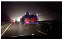
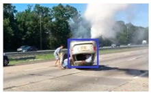
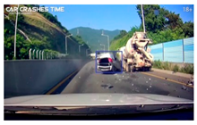
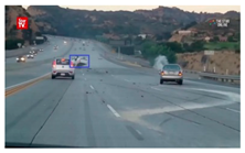
In this study, the severity of an accident was determined by classifying accidents based on whether a car is damaged or has overturned. Accidents involving overturned cars, in which a large impact upon collision causes a car to destabilize and overturn, are more likely to become fatal and lead to higher death rates as the driver may be flung out of the car or become stuck inside. This study on accident detection was conducted in the context of highways. Due to higher car speeds on highways relative to other road types, there are stricter requirements with regard to the timeliness of object detection.

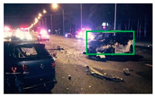
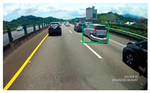
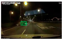
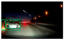
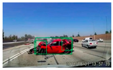
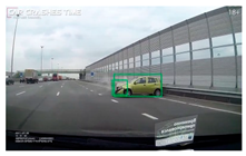
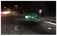
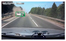
With the abovementioned objectives in mind, dashcam images were primarily used in this study for training and testing datasets. An accident recognition and classification system based on the YOLOv3 algorithm was used to classify serious highway accidents, thus enhancing the objectivity of accident severity classification. In addition, the Canny edge detection algorithm was used to elicit the boundary of an object in an image. By delineating the boundary of a car, the neural network learning process becomes easier to perform. The results demonstrated that the mean average precision (mAP) of the proposed model, following tests based on dashcam images, was 62.60%; and when single high-resolution images were used, the model’s mAP reached up to 72.08%. When comparing the proposed model with a benchmark model, two abovementioned accident types were combined to allow the proposed model to produce binary classification outputs (i.e., non-occurrence and occurrence of an accident). The HDCA-CS was then applied to the two models, and testing was conducted using single high-resolution images. At 76.42%, the mAP of the proposed model outperformed the benchmark model’s 75.18%; and if we were to apply the proposed model to only test scenarios in which an accident has occurred, its performance would be even better relative to the benchmark. These results show the superiority of the proposed model compared to other existing models.

1.4. Contributions

The contributions of this study are as follows:

• Classification of accidents:

The two objectives of detecting and classifying highway accidents are to preliminarily assess the severity of an accident and to facilitate preparations for subsequent rescue operations. Lives may be lost if an accident remains unclassified at the time of the report or if the severity of an accident was misreported, resulting in rescue workers arriving at the scene without the appropriate equipment for the rescue operation.

• Increasing data volume through Canny:

The most important aspect of the training process has a balanced dataset. As there is a lack of accident-related data, which are often maintained as criminal records, and it is difficult to purchase data in the same way that large companies do, the data used in this study was only obtained from online platforms. To make up for the gap between datasets, the Canny algorithm was introduced into the training set along with images of cars with drawn boundaries, thus adding more diversity to the learning process. Meanwhile, the Canny algorithm was used to delineate the boundary of a car in an image, and thereby, facilitate the neural network learning process.

• Realistic simulation:

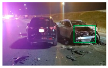
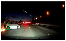
In comparison with other studies that input high-resolution images of accidents into their models for training, this study directly used segmented images from dashcam videos for training. This increases the model’s sense of realism as an actual accident is usually accompanied by smoke and dust, and recorded as blurry and shaky footage. Weather conditions are also reflected in the model by including road conditions, such as rain and fog.

• HDCA-CS (Highway Dashcam Car Accident for Classification System) dataset:

This study mainly obtained dashcam videos from online platforms, appropriately segmented the videos into images, and extracted the accident-relevant segments. The dataset was named Highway Dashcam Car Accident for Classification System (HDCA-CS). This dataset is a requisite for simulation and was developed to enhance model learning.

1.5. Organization

The subsequent sections of this study are structured as follows: Section 2 is a review of the relevant literature. Section 3 describes the research methods, model design, anticipated sequences of an accident, training approaches, utilization of the Canny algorithm, and model classification. Section 4 presents the test results of the model, as well as a discussion and analysis of the results. Section 5 presents the conclusions and potential research directions.

2. Related Work

In this section, we shall conduct a more in-depth review of accident detection-related studies, including studies that performed conceptual comparisons of accidents [16,17]; a study that utilized the Histogram of Oriented Gradient (HOG) feature and the Support Vector Machine (SVM) as learning approaches for accident detection [18]; studies that applied YOLO-based models as a learning method for accident detection [19,20,21,22]; a study that combined SVM and YOLO for accident detection [23]; a study that investigated the prediction of accidents [24]; studies that utilized the accelerometer and gyroscope inside a smartphone in combination with other factors to determine whether an accident would occur [25,26]; studies that compared and studied image processing techniques [27,28]; and studies about the application of the Canny edge detection algorithm [29,30].

Sonal and Suman [16] adopted data mining and machine learning approaches to consolidate accident-related data. The authors incorporated a linear regression into their algorithm and compared the occurrences of accidents by examining details, such as location, time, age, gender, and even impact speed. Hence, the authors provided diverse perspectives on the factors that contribute to accidents. Naqvi and Tiwari [17] explored accidents involving two-wheel heavy motorcycles that occurred on highways in India. The aim of that study was to determine the type of crash, vehicles involved, number of lanes affected, and the time of the accident; and the results were simulated using binary logistic regression. The study mostly focused on heavy motorcycles and did not elaborate on four-wheel passenger cars.

In a study on automatic road accident detection systems conducted by Ravindran et al. [18], a supervised learning approach that combined the HOG feature with SVM classifiers was proposed. It focused on two types of cars—cars that were involved in an accident and cars that were not involved in an accident. The detection system comprised of three stages. In the first stage, a median filter was used for image noise reduction, and the HOG feature was used for feature extraction, followed by training with an SVM. Next, the local binary pattern and grey level co-occurrence matrix features were used to enhance the performance of the system. Finally, to identify damaged cars more accurately, a three-level SVM classifier was employed to detect three types of car parts (wheels, headlights, and hoods). Gour and Kanskar [19] employed an optimized-YOLO algorithm to detect road accidents. Relative to YOLOv3, the optimized-YOLO algorithm only has 24 convolutional layers, which is easier to train. In terms of data collection, the algorithm was trained using 500 images of accidents with only a single class, i.e., damaged cars. In 2020, Wang et al. [20] proposed the Retinex algorithm for enhancing the quality of images taken under low-visibility conditions (e.g., rain, nighttime, and fog). The environments examined were diverse and complex road sections. The YOLO v3 algorithm was used for accident detection training with respect to road accidents that involve pedestrians, cyclists, motorcyclists, and car drivers. Lastly, the algorithm was tested by using roadside closed-circuit television (CCTV) footage. Tian et al. [21] developed a dataset named Car Accident Detection for Cooperative Vehicle Infrastructure System dataset (CAD-CVIS) to train a YOLO deep learning model named YOLO-CA. The dataset mainly consisted of images from roadside CVIS-based CCTV footage, and was designed with the aim of enhancing the accuracy of accident detection. Furthermore, in congested urban areas, traffic flow monitoring is a salient indicator. Babu et al. [22] developed a detection framework that consists of three components: data collection, object detection, and result generation. During data collection, roadside CCTV footages were segmented into images, and YOLO was used as a tool for traffic flow detection. Finally, during result generation, Opencv+TensorFlow API was utilized to detect the speed, color, and type of the car that appears in an image. Arceda et al. [23] studied high-speed car crashes by employing the YOLO algorithm as a detection tool and utilizing the algorithm proposed in another study [31] to track down each car in an image. In the final step, an accident was validated using a Violent Flow descriptor and SVM, and the dataset comprised CCTV footage.

Chan et al. [24] conducted a study on accident anticipation that took into consideration the wide use of dashcams in our daily lives and potential application as a rational means of anticipating whether an accident will occur in front of a driver. The authors in that study proposed the dynamic-spatial-attention recurrent neural network for anticipating accidents using dashcam videos. Furthermore, several recent studies have used smartphones for real-time accident analysis and reporting. Smartphones are a necessity nowadays, and it is extremely common to see people carrying smartphones. If smartphones can be used to identify accidents, equipment costs can be reduced. Sharma et al. [25] advocated the use of smartphones for automatic accident detection, to reduce delays in accident reporting. In the proposed method, accidents were identified by utilizing special circumstances related to the time of the accident. As accidents are usually accompanied by high acceleration and loud crashes, the authors of that study adopted acceleration and the sound of crashes as a basis of accident determination and used them to develop the collision index (CI). Then, the CI intervals were used as an indirect means of assessing the severity of an accident. In a similar vein, Yee and Lau [26] also used smartphones for accident detection. These researchers used the global positioning system (GPS) and accelerometer in a smartphone for simulations and developed the vehicle collision detection framework. GPS was used to measure car speed, while the accelerometer was used to calculate the acceleration force.

In the field of image processing, edge detection algorithms are an important technique. Acharjya et al. [27] compared many edge detection algorithms (Sobel, Roberts, Prewitt, Laplacian of Gaussian, and Canny) and revealed that Canny performed the best, as validated through the peak signal-to-noise ratio and the mean squared error results. S. Singh and R. Singh [28] applied various methods to compare the Sobel and Canny algorithms, which are both commonly-used edge detection algorithms. They clarified that neither algorithm was superior to the other and differed in terms of their scopes of application, that is, both algorithms have their distinct advantages when they are used in different situations. The Canny algorithm has been applied in the field of image recognition. With regard to traffic congestion in urban areas, Tahmid and Hossain [29] proposed a smart traffic control system and used the Canny algorithm for image segmentation during image processing. Thereafter, methods from other studies were added to that system to detect vehicles on the road. Low et al. [30] employed the Canny algorithm for road lane detection, contributing toward efforts to implement self-driving cars in the future.

Consolidating the aforementioned literature, we can observe that the models and systematic theories proposed were mainly used for research on accident detection, and that there is a dearth of research on accident classification. Furthermore, the datasets in most of the studies were built using CCTV footage instead of dashcam footage.

Table 2. Comparison of angles of view.

	Method	Dashcam (Used in This Study)	CCTV (Used in Many Studies)
Comparison
Benefits		Positioned close to a driver and assists in driver safety Records views from various angles; more data can be stored Affordable and can be acquired by anyone	Takes high-angle footage and has a wide field of vision Higher accuracy of data transfer as data transmission between cars is not required
Drawbacks		Lacks a wide field of vision; detections cannot be made if the view of an accident ahead is blocked by other vehicles Data transfer is harder to achieve, due to more factors that require consideration	Blind spots arise from the gaps between areas covered by different CCTVs Costlier and more difficult to install Limited to a single field of view, which lowers the volume of data collected
Suitable applications		Highways	County and city roads

presents the advantages and disadvantages of these two approaches and their applicable settings. In this study, the HDCA-CS dataset consisted mostly of dashcam images.

3. Model Design

3.1. Description of Scenarios

As shown in Figure 2, as Car A moves along a highway, the smart detector on the dashcam onboard detects an overturned car in front and labels it in the video (see the inlet picture titled Car A Dashcam video scene). Then, Car A would intelligently assist the driver to brake in time instead of performing sudden braking, which could lead to skidding and secondary accidents. At the same time, the accident is relayed to other cars behind (Cars B and C) using wireless messaging. Lastly, it is recommended that the accident message is sent through 5th generation mobile network (5G) Internet of Vehicles (IoV) [32] to a base station nearby, which in turn consolidates the data and sends it to the cloud platform of the police and hospitals, allowing them to deploy rescue teams. This study focuses on the detection and classification of accidents, and as for the other topics that were brought up (e.g., base station transmission [33]), they could be further explored in future studies.

In Taiwan, there is no defined standard for classifying car accidents, while the American government has stipulated regulations governing the legal responsibilities associated with different types of accidents [34]. A rollover, which is a serious type of accident, happens when the impact of the collision is great enough to overturn a car. Rollovers account for more fatalities (35%) than any other type of accident. In this study, rollovers are defined as accidents involving overturned cars. While there are many other types of accidents, such as head-on collisions, lane crossovers, multi-vehicle crashes, for the sake of simplicity, this study summarized these accidents as accidents involving damaged cars. Therefore, based on the statements above, accidents are categorized into two types in this study, to serve as a standard for the preliminary classification of the severity of an accident. More specifically, the condition of a car can be categorized into one of the following three types:

• Class A: vehicle
  A car without any damage is defined as a vehicle.
• Class B: damaged car
  A car with its hood, bumper, headlights, and other front or back parts damaged, due to an accident to the point of deformity and becomes different from a normal car, is defined as a damaged car. Accidents that cause defects in the cars involved are minor and have a lower injury rate.
• Class C: overturned car
  A car that overturns, due to a serious accident involving only itself (single-vehicle collision) or a collision with another car, is defined as an overturned car. In either case, the high speed of the car upon impact is great enough to structurally destabilize and overturn the car. Consequently, drivers become stuck inside, and this type of accident has a high death rate.

Based on the classification above, priorities in subsequent data treatment can be defined based on the concept of 5G IoV. If the base station receives a Class B and a Class C accident at the same time, it will determine that the Class C accident is more severe than the Class B accident, and would send a message regarding the Class C accident to rescue workers first, followed by the Class B accident.

3.2. Design of the Overall Process Framework

As shown in Figure 3, the overall process of the model consists of three steps: Data preparation, model training, and model mAP testing. The test procedures and relevant theories will be described later. The data preparation step further consists of a training set and a test set. The benefits and drawbacks of different methods of collecting data for the training set are listed in

Table 3. Comparison of data collection methods.

	Method	Video-Segmented Single Images (The Main Data Collection Method Proposed in this Study; Some Original Single High-Resolution Images Were Included as Well)	Single High-Resolution Images (Data Collection Method Used in Most Studies)
Comparison
Benefits		When an accident occurs, the angles at which the car becomes damaged or overturned over time can be accurately identified. Allows the model to learn about an accident from various angles, thus increasing the diversity of accident types. There are often clues that lead to an accident, such as a skidding car. Video segmentation enables one to screen the features of many accidents before they occur, thus enabling the model to learn how to predict an accident.	Models are easy to train, due to the high quality of the images. Focuses on the distinct external features of a car, enabling a model to learn the changes in a car’s exterior before and after an accident. No further screening of details is required after images have been collected.
Drawbacks		Videos downloaded from a free online platform have lower qualities, which increases the difficulty of model training. Segmenting images of accidents from a video requires screening, which consumes human resources and time.	A single accident image does not contain much information on an accident and lacks many accident features. Data collection is more difficult and lacks diversity. Real-time accident features cannot be presented
Suitable applications		Acquires real-time information at the moment when an accident occurs. Applicable for real-time dynamic recognitions.	Detection of roadside accidents that have already occurred. Applicable for static recognition.

.

3.2.1. Data Preparation

As the name suggests, the aim of this step is to prepare the data for model learning and training. To facilitate future studies, three smaller components are further defined: (1) A training set consisting of dashcam images; (2) A training set consisting of single high-resolution images of accidents; and (3) A test set used for model testing.

(1)

Training set consisting of dashcam images

The data here consists of sets of images segmented from a dashcam video at 0.5-s time intervals. The data were mainly obtained from two sources: (a) Relevant images were downloaded from Google Images by inputting keywords; (b) Videos were downloaded from YouTube and then segmented into images. All the images were in JPG format.

(2)

Training set consisting of single high-resolution images of accidents

With different model designs in mind, this training set aimed to elicit the boundary of a car involved in an accident. The dataset consists of single high-resolution images of accidents that have been processed by the Canny edge detection algorithm.

(3)

Test set for model testing

The set of images used for testing the mAP of the model was the same as that of the training set.

3.2.2. Model Training

In model training, four different types of the model designs (M1, M2, M3, and M4) were established. More details will be provided in the subsequent text. The number of epochs for model training was 500 in all model designs. After 500 rounds of training, the weights and biases of the neurons will be produced.

3.2.3. Model mAP Testing

In model mAP testing, the weights and biases produced in the preceding step are introduced into the model for testing.

3.3. Principles of mAP Testing

In model testing, an indicator that evaluates the learning outcomes of a model is required to determine whether the model is good or bad. The mAP is an indicator commonly used to evaluate how good a model is. Meanwhile, it is noted that True Positive (TP) indicates that the model correctly identified an actual target, and False Positive (FP) indicates that the model identified an actual non-target instead of an actual target. In target detection, the Intersection-over-Union (IoU) value of the predicted Bbox and the ground truth box is calculated. If the IoU exceeds a certain predefined value, the detection is a TP, and FP if otherwise. Here, precision is defined as

$$\mathrm{Precision} =\frac{\mathrm{TP}}{\mathrm{TP}+\mathrm{FP}}$$

(1)

Precision, in terms of single predictions, is the ratio of correctly predicted targets to the total number of predictions. In this study, there were 340 images in the test set, and hence, the AP of a model can be derived after 340 tests have been performed

$$\mathrm{AP}=\frac{{\displaystyle \sum \mathrm{Precision}}}{340}$$

(2)

Furthermore, given that three types of accidents were taken into account in this study, then the mAP of the three types of accidents can be written as

$$\mathrm{mAP}=\frac{{\displaystyle \sum \mathrm{AP}}}{3}$$

(3)

In terms of calculations based on each type of accident, i.e., calculations on Class B and Class C accidents, then the accident mAP can be written as

$$\mathrm{Accident} \mathrm{mAP}=\frac{{\displaystyle \sum \mathrm{AP}} \mathrm{of} \mathrm{Class} \mathrm{B} \mathrm{accidents}+{\displaystyle \sum \mathrm{AP}} \mathrm{of} \mathrm{Class} \mathrm{C} \mathrm{accidents}}{2}$$

(4)

3.4. Labeling of Car Types and Design of Subtypes

The LabelImg tool was used to label images in this study. LabelImg outputs the car types in each frame according to their labels, as well as the coordinates of the four corners of the frame, which are then converted to VOC format. The YOLOv3 algorithm begins to learn according to the pixels in the frame.

3.4.1. Labeling Class A Scenarios

As shown in the images in

Table 4. Labeling Class A scenarios. (Original images taken from Car Crashes Time [35]).

, red frames are used to label normal cars.

3.4.2. Labeling Class B Scenarios

Green frames are used to label damaged cars, which are further divided into three subclasses.

Class B1: Car Parts Frame

As shown in the images in

Table 5. Labeling Class B1 scenarios. (original images taken from Car Crashes Time [35]).

, only damaged car parts, such as the front, rear, sides, or other accessories, are labeled. This method is similar to that of the aforementioned study [18], which describes a detection method based on damaged car parts.

Class B2: Car Body Frame

As shown in the images in

Table 6. Labeling Class B2 scenarios. (original images taken from Car Crashes Time [35]).

, entire damaged cars are labeled. This method is a more common approach in accident detection [23].

Class B3: Composite Frame

Class B3 is defined as the union of Class B1 and Class B2 labels (B1$\cup$B2), as shown in the images in

Table 7. Labeling Class B3 scenarios. (original images taken from Car Crashes Time [35]).

. This method is an original approach.

3.4.3. Labeling Class C Scenarios

As shown in the images in

Table 8. Labeling Class C scenarios. (original images taken from Car Crashes Time [35]).

, blue frames are used to label overturned cars.

3.5. Incorporating the Canny Edge Detection Algorithm

As mentioned in Section 1, image processing plays a salient role in object detection. Compared to many other edge detection algorithms, the Canny edge detection algorithm has a remarkably good edge detection ability in the field of image processing. Therefore, in this section, we used the Canny edge detection algorithm to process single high-resolution images of accidents. On the one hand, this removes unnecessary non-accident backgrounds and extracts the features of an accident from a single image; on the other hand, it overcomes the problem of an insufficient dataset volume. Prior to performing Canny edge detection, the position of targets in the original set of single high-resolution images of accidents was labeled via LabelImg. The process of the Canny edge detection algorithm consists of gray image scaling, Gaussian blurring, calculating the gradient intensity and direction, edge thinning, and determining the double threshold values.

The first step is to convert the image into a gray level image via the formula below:

$$\mathrm{Gray} =\frac{\mathrm{R} + \mathrm{G} + \mathrm{B}}{3}$$

(5)

However, as humans, our color vision acuity differ from one another, weights were allocated based on acuity, and the formula was modified as

$$\mathrm{Gray}\_\mathrm{modified} = 0.299\mathrm{R} + 0.587\mathrm{G} + 0.114\mathrm{B}$$

(6)

Gaussian blurring utilizes kernels with Gaussian features to convolve an image. Therefore, the intention of utilizing Gaussian blurring is because Gaussian functions have rotational symmetry. When Gaussian functions are used to smoothen an image, the results will show that the smoothing level is equal in all directions, and hence, in subsequent edge detection operations, smoothing is not biased toward the edges of an image in a certain direction. Moreover, the weight of a pixel decreases when its distance from the Gaussian center point increases. The kernel size of a Gaussian filter also influences the results of the Canny algorithm. A smaller filter produces less blurring effects, which enables the detection of lines that are finer and have more obvious changes, while a larger filter produces more blurring effects. Based on various considerations, this study applied a Gaussian filter with a kernel size of 5 to reduce the noise of an image and decrease the layers of details, thereby filtering the unnecessary details out and outlining the target object.

We define I as the pixel matrix of an image and $\otimes$ as the convolution symbol. Then, convolution was performed on an image using the Sobel operator. The first derivatives in the horizontal ($G_x$) and the vertical ($G_y$) directions were derived, followed by the gradient angle $\theta$. $G_x$, $G_y$, and $\theta$ are represented, respectively, as follows:

$$G_x=\left[\begin{array}{ccc}-1& 0& +1\\ -2& 0& +2\\ -1& 0& +1\end{array}\right]\otimes I,$$

(7)

$$G_y=\left[\begin{array}{ccc}-1& -2& -1\\ 0& 0& 0\\ +1& +2& +1\end{array}\right]\otimes I,$$

(8)

$$\theta ={\tan }^{-1}\left(\frac{G_y}{G_x}\right),$$

(9)

Then, non-maximum suppression (NMS) was used to compare each pixel along the derived direction of $\theta$, to check whether a pixel value was the maximum along the gradient direction. Such a pixel has a higher retained intensity than those of its neighboring pixels. This process is known as edge thinning (as depicted in Figure 4).

Lastly, the double thresholds minVal (T1) and maxVal (T2) were used to screen for actual edges. Figure 5 shows an image with edges. Point A has a value higher than T2 and is a point on an actual edge. Even though the value of Point C is between the two thresholds, it is connected to Point A, and is also regarded as a point on edge. The value of Point B is lower than T2, is not connected to any point, and is regarded as a non-edge point. Points smaller than T1 are omitted. This was done to connect different edges, as using a single threshold could result in an image with many intermittent edge lines.

If T2 is set too high, important information in an image may be left out; if T1 is set too low, the edges of details may be drawn. This study used the Canny algorithm because the desired boundary of a car in an image can be retained, and other details in the background can be omitted. Therefore, selecting the suitable thresholds prior to applying the Canny edge detection algorithm to an image is important for obtaining desired results. This study employed the averaging method, in which optimum adjustments were conducted based on 20 images with high resolutions selected from the dataset. The reason for using these higher resolution images is because the features of an accident can be fully presented after performing the Canny edge detection algorithm. If low-resolution images were used instead, the features cannot be presented effectively after edge thinning, and adjusting T1 and T2 would become meaningless. The adjusted values of T1 and T2 based on the 20 test images are listed in

Table 9. Adjusted thresholds in the Canny dataset.

No.	T1 (pixel value)	T2 (pixel value)	No.	T1 (pixel value)	T2 (pixel value)
1	10	98	11	128	250
2	17	140	12	116	220
3	51	106	13	170	250
4	139	255	14	21	213
5	62	229	15	43	156
6	31	106	16	55	191
7	82	191	17	32	238
8	120	210	18	68	242
9	60	196	19	40	166
10	48	163	20	65	104

. The optimum values were derived from the mean of the sum of the 20 adjustments, which was 60 and 164 for T1 and T2, respectively. The optimum values were then substituted into the other images in the dataset for Canny edge detection. To comply with the concept of data cleaning, we selected images from the dataset that were suitably-adjusted. After the Class B and Class C scenarios had undergone Canny edge detection algorithm processing, 402 images were added into the model, which corresponded to a 33% increase in the initial number of images (796) in the dataset. Further details will be provided in Section 4.

3.6. Model Classification

As mentioned in Section 3.4.2, Class B consisted of three different design methods (i.e., B1, B2, and B3). We selected the design method with the best mAP after comparing the three design methods (which was Class B2; the data is presented in Section 4) and then added it to the single high-resolution images dataset that were processed through Canny. As a result, four types of models were designed, namely, Models M1, M2, M3, and M4. Model M1 contained a dataset that consisted of Classes A, B1, and C data; Model M2 contained a dataset that consisted of Classes A, B2, and C data; Model M3 contained a dataset that consisted of Classes A, B3, and C data; Model M4 contained a dataset that consisted of Classes A, B2, C data, as well as Canny-processed single high-resolution images. These models are summarized in

Table 10. Model classification.

Model	M1	M2	M3	M4
Dataset	A + B1 + C	A + B2 + C	A + B3 + C	A + B2 + C + Canny

.

4. Results and Discussion

4.1. Software and Hardware Preparation and Consolidation of Training Data

4.1.1. Software and Hardware Preparation

This study employed the Keras version of the YOLOv3 algorithm [36]. The computer hardware and device configuration are shown in

Table 11. Hardware configuration.

Processor	Intel® Core™ i5-8500CPU @ 3.00GHZ *6
Display card	NVIDIA GeForce GTX 1060 6GB
Operating system	Windows 10
Memory	8GB (RAM)

.

4.1.2. Consolidation of Training Sets

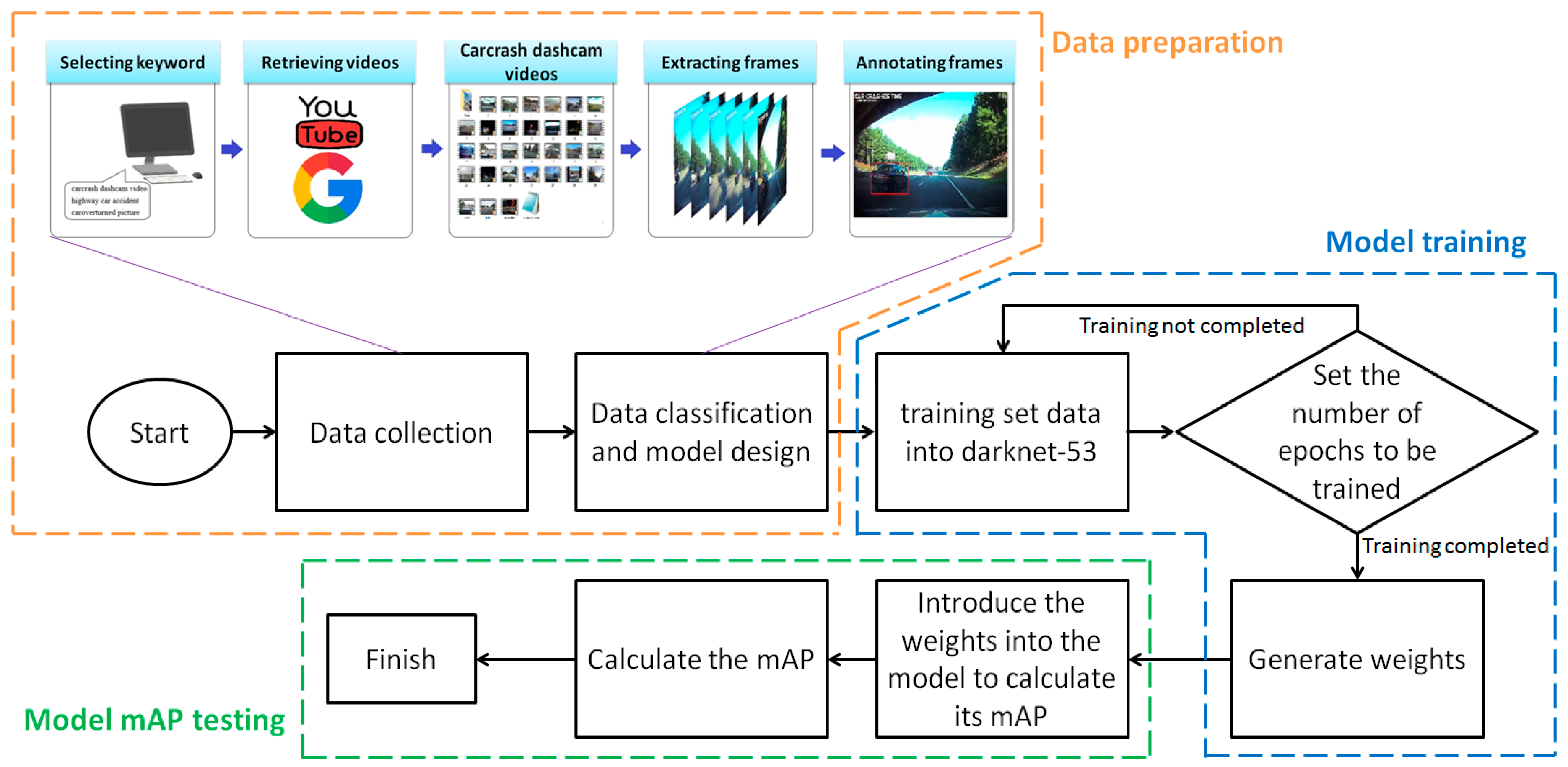
The Classes A, B, and C datasets were sourced from the same “Car” category in the PASCAL VOC dataset. Here, during model learning, the emphasis was placed on the changes in the exterior features of a car. Due to the difficulty of obtaining first-hand accident information, the labeling method in the text refers to the labeling of all the possible samples (this approach is more feasible and effective given that it is difficult to obtain first-hand accident information). Therefore, the sample size of the Class A set was naturally larger than those of the Class B and Class C sets. Under these conditions, even though the model had more learning opportunities with respect to the Class A set, the likelihood of misrecognizing a Class A scenario as a Class B or Class C scenario can be reduced to a certain extent. This also indirectly increases the accuracy of the model to correctly recognize Class B or Class C scenarios. Lastly, to increase the features and volume of the accident dataset, the original single high-resolution images of accidents were first labeled via LabelImg and then subjected to Canny edge detection. The number of images in each class of the dataset is summarized in

Table 12. The number of images in each training set and the total number of images.

	Images that Do Not Contain an Accident	Images that Contain an Accident		Total Number of Images
Category	Class A	Class B	Class C	Total dataset
Original number of images	3141	796		3997
Number of images added after Canny detection (Labeling followed by Canny detection)	0	402		402
Total number of images	3141	1198		4339

. It should be pointed out that YOLOv3 will enhance the training set during the training process, making adjustments with respect to saturation, exposure, and hue, which were set to 1.5, 1.5, and 0.1, respectively. To determine how the use of Canny detection benefits Model M4, we incorporated another model (i.e., a Model M4 without Canny detection) and compared it to Model M4. The Model M4 without Canny detection was trained using the training set consisting of dashcam images and the training set consisting of single high-resolution images of accidents (i.e., not subjected to Canny detection).

4.2. Statistics of Test Results

Firstly, the LabelImg tool was used to label the ground truths of an additional 340 untrained images (not included in Table 12). The dataset also took into account various weather conditions and environmental factors, to increase the diversity of testing instead of merely doing so for the sake of data acquisition. Then the weights derived from training were introduced into the model for testing. The IoU threshold was defined as 0.5 in this study. A detection was considered as a true detection if the IoU exceeded 0.5, and a false detection if otherwise. The cutoff point of 0.5 was established based on the findings of the aforementioned study [9], which revealed that humans are unable to discern the differences between IoUs ranging from 0.3 to 0.5.

The statistics of the test results are presented in

Table 13. Statistics of the test results of each model.

Overall Detection Results for Model M1	Ground Truth Statistics for Model M1
Overall detection results for Model M2	Ground truth statistics for Model M2
Overall detection results for Model M3	Ground truth statistics for Model M3
Overall detection results for Model M4	Ground truth statistics for Model M4
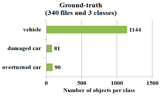
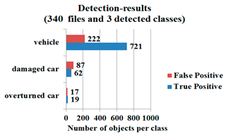
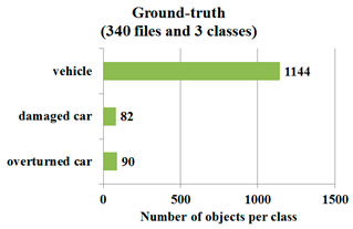
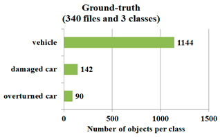
Overall detection results for Model M4 without Canny detection	Ground truth statistics for Model M4 without Canny detection

. With regard to the number of ground truths, Class A and Class C scenarios had 1144 and 90 ground truths, respectively. In other words, the 340 test images contained 1144 normal cars and 90 overturned cars. Since Class B was divided into three subclasses (with different design methods), naturally, there were differences between the three sub-methods in terms of quantity.

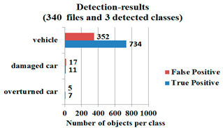
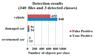
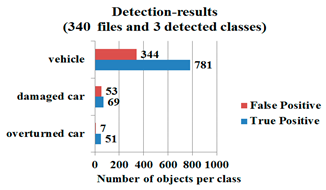
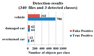
The statistical results presented here are mainly used to examine the effectiveness of the models in terms of the rate of target detection. In the case of Model M1, only 734 cars were detected, and the IoU of the remaining 352 detection results was smaller than 0.5. Based on the experimental results, the FP of a model in relation to detecting Class A scenarios refers to the outcome in which the model had failed to detect an actual accident. On practical terms, the model is regarded as having neglected an accident and was unable to report the actual situation; the FP of a model in detecting Classes B and C scenarios refers to the outcome in which the model had detected an accident that had not to occur in reality. On practical terms, the model is regarded as having misreported an accident or made an error in accident classification. The FPs of Models M1 and M2 in detecting Classes B and C scenarios were greater than their TPs. In other words, these two models had a higher error rate. Conversely, the FPs of Models M3, M4, and M4 without Canny detection in relation to detecting Classes B and C scenarios were smaller than the TPs, which means that these two models had a lower error rate relative to Models M1 and M2. This also means that Models M3 and M4 had higher stabilities.

Of all the models, Model M2 had the lowest number of FPs in detecting Class A scenarios. This shows that Model M2 was superior to the other models in terms of detecting Class A scenarios. With regard to Models M1, M2, and M3, which had similar datasets, but differed in terms of the Class B design methods, the results indicated that Model M2 had a higher ability to detect a higher number of actual accidents. Since Models M4 and M4 without Canny detection were based on the design method of Model M2 in which the Canny-processed single high-resolution images were added into the dataset, it had better test results in terms of detecting Classes B and C scenarios compared to Model M2. In other words, it had a higher number of TPs and less FPs. Therefore, it is evident that using the dataset containing Canny-processed single high-resolution images was extremely beneficial for model training.

The detection results indicated that Model M4 performed better than the Model M4 without Canny detection. Specifically, the two models’ performance was virtually identical when detecting Class A scenarios, but differed when detecting Class B and Class C scenarios. Compared to the Model M4 without Canny detection, Model M4 produced more TP results and fewer FP results when detecting Class B and Class C scenarios. This indicates that the addition of Canny detection can effectively enhance single high-resolution image datasets for model training, and thereby, improve a model’s performance.

4.3. mAP Results

Table 14. Mean average precision (mAP) results of various models.

M1 mAP: 24.89%	M2 mAP: 44.60%
M3 mAP: 36.16%	M4 mAP: 62.60%
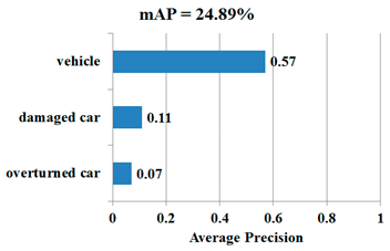
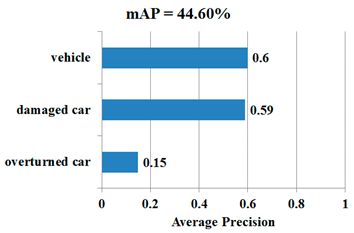
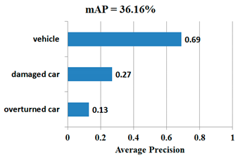
M4 without Canny detection mAP: 56.67%

presents the mAP results of each model derived from tests based on dashcam images. The mAP test results revealed that Model M4 had the best mAP among all models at 62.60%, while Model M1 had the lowest mAP at 24.89%, which was far lower than the other models. In other terms, Model M1 was less superior than the other models in terms of model design method.

With regard to detecting Class A scenarios, all four models had produced decent results. With regard to detecting Class B scenarios, the AP of Model M2 (in which a damaged car is labeled in its entirety) was up to 59%. M2 also had the best mAP test result out of Models M1, M2, and M3. Even though the functionality of Model M3, which combines the designs of Models M1 and M2, cannot be presented completely in the results, Model M3 was able to label the cars that were involved in an accident along with the damaged car parts and the moment of impact. In other words, even though Model M3 did not perform better than the other models in terms of the design methods of detecting Class B scenarios, it was able to show more detailed information about damaged cars.

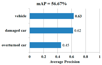
Moreover, when processing the original number of datasets, Models M1, M2, and M3 had marginal differences in detecting Class C scenarios. The Model M4 without Canny detection was created by additionally training Model M2 (its mAP is 44.60%) using single high-resolution images of accidents. The mAP of this model was 56.67%, representing an increase of about 12%. It is clear that the Model M4 without Canny detection is better than Model M2 at identifying different types of scenarios, particularly Class C scenarios (i.e., overturned car) for which the improvement was significant. With the inclusion of Canny detection for enhanced model training, Model M4 was able to outperform the Model M4 without Canny detection, achieving an mAP that was about 6% higher and demonstrating the benefits of effective Canny detection integration. Following the additional use of Canny-processed single high-resolution images of accidents, Model M4 showed a significant improvement in detecting Class B and Class C scenarios. In addition, the model’s AP of detecting Class B scenarios was up to 73%, which exceeded that of detecting Class A scenarios. Model M4 can represent the novel design method proposed in this study, as the results demonstrate that adding the Canny algorithm into image processing had effectively increased the mAP of the model.

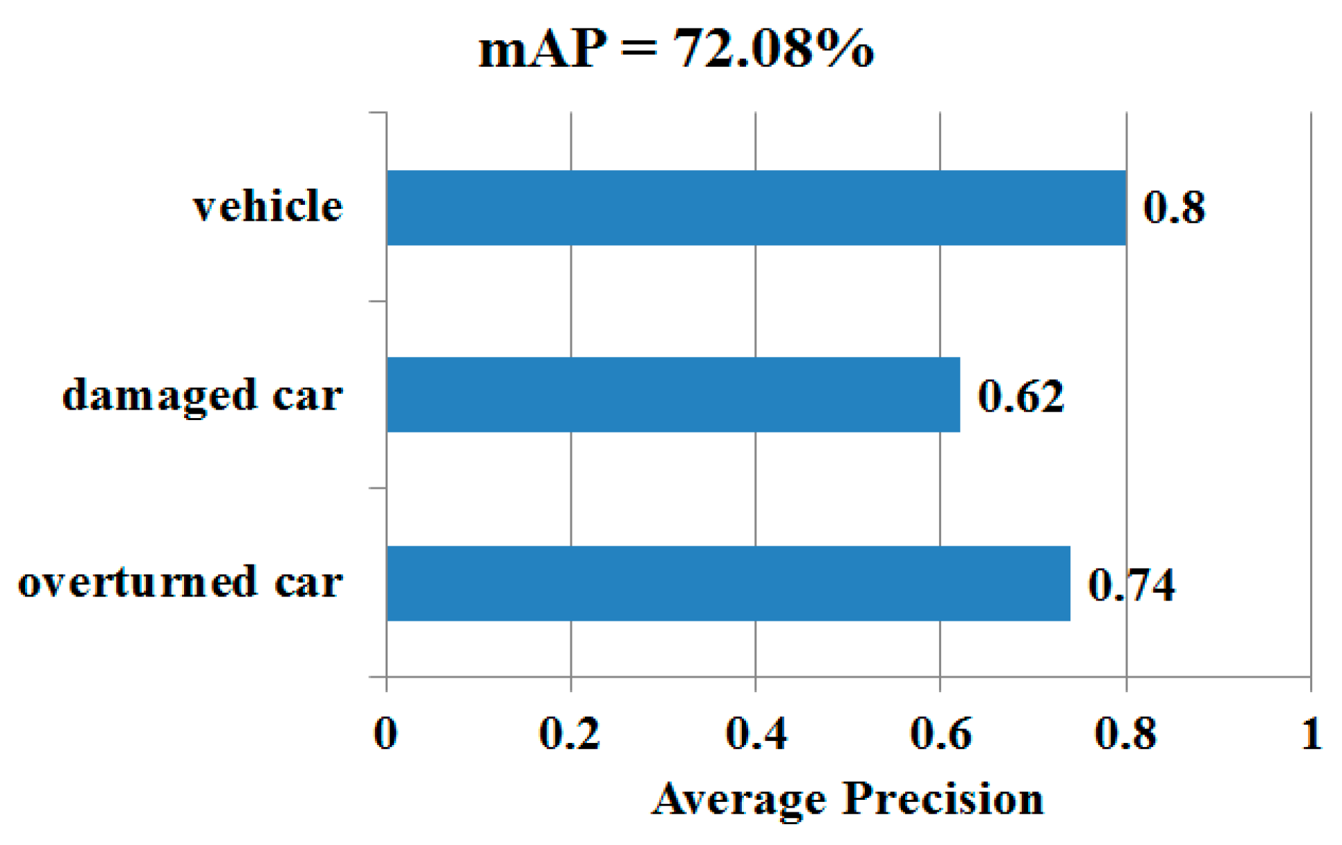
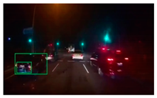
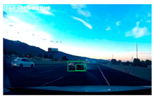
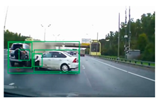
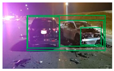
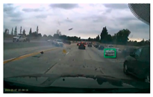
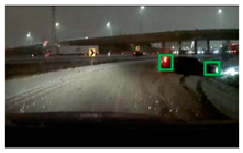
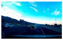
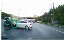
This study also performed tests using single high-resolution images. As shown in Figure 6, using the best-performing model (M4) yielded an mAP of up to 72.08%. Even though this study was mainly based on the angle of view of dashcams, however, for the sake of increasing the diversity of the dataset, single high-resolution images were also used as a supplementary, which was proven to be effective.

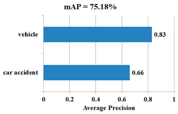
To demonstrate the superiority of Model M4, we compared its mAP performance to that of the model (i.e., YOLO-CA) used in an aforementioned study [21]. The YOLO-CA model was trained using the HDCA-CS dataset during the training phase, and later tested using single high-resolution images. In that study, binary classification was applied to YOLO-CA’s outputs (i.e., non-occurrence and occurrence of an accident). For the purpose of performing comparisons with YOLO-CA, we converted Model M4′s ternary category classification framework into a binary one to match the binary outputs produced by YOLO-CA. Specifically, we kept the “vehicle” category unchanged since it corresponded to YOLO-CA’s “no accident” category; but merged the “damaged car” and “overturned car” categories and labeled the merged category as “car accident,” such that it corresponded to YOLO-CA’s approach of using one category to cover all scenarios in which an accident has occurred. The test results (

Table 15. YOLO-CA [21] and Model M4 mAP results.

YOLO-CA [21] mAP: 75.18%	M4 mAP: 76.42%

) indicated that Model M4 performed better with an mAP of 76.42% relative to YOLO-CA’s mAP of 75.18%. A closer look at the results revealed that Model M4 and YOLO-CA’s APs for the “vehicle” category were 81% and 83%, respectively. This finding could be attributed to the fact that the HDCA-CS training set consisted primarily of dashcam data. This is because most cars are treated as small objects from the dashcam perspective, and YOLO-CA is a model designed to enhance the detection of small target objects and achieve better performance in terms of small object detection. However, from the dashcam perspective, it is difficult in practice to detect an accident that has occurred far in the distance, and even a driver would find it challenging to determine whether a car is overturned or merely damaged in this situation. In other words, the human eyes are often only able to accurately identify car accident scenarios when the accident occurs at a location closer to the dashcam. Therefore, car accidents (involving damaged or overturned cars) in the collected dataset comprised mostly medium-sized objects. While YOLO-CA does not enhance the detection of medium-sized objects, the Canny edge detection algorithm used in our study enables data enhancement; that is, training is carried out to achieve enhanced identification with respect to the relevant objects found in single high-resolution images of car accidents. Judging by the car accident scenario test results, Model M4 performed better with an AP of 71% as opposed to YOLO-CA’s AP of 66%, and based on the above observations and reasons, Model M4 is superior to existing methods in detecting car accident scenarios.

4.4. Discussion of Results

Based on the results of the four models in this study, all models had a qualified AP in terms of Class A scenario detection, and the models for M1, M2, and M3 had higher Class A APs compared to the models used for detecting Classes B and C scenarios. This result was expected, due to the sufficient data volume, which allowed the model to study a diverse range of data. Adding images processed by the Canny edge detection algorithm into the dataset of Model M4 allowed it to perform better than the other models in terms of Class B and Class C scenario detection; therefore, the inclusion of images processed by the Canny edge detection algorithm had increased the accuracy of the model in detecting Class B and Class C scenarios.

Based on the results, and owing to the design method used for detecting Class B scenarios (only damaged car parts were framed), Model M1 had a remarkably poorer performance than the other models. Therefore, it can be deduced that this model was unable to allow a machine to learn the actual meaning of a damaged car part. This is because the model only labels damaged car parts in an image, and there is no defined standard for assessing the severity of car damage. If we are unable to establish standards for determining damage severity (e.g., whether the damage is severe or light), the machine would also not be able to learn and define damage severity.

Even though it might seem that this study only modified the design methods of Class B scenarios, in reality, the design methods of Class B scenarios are associated with the overall accident classification to a certain extent. In other words, the design of the methods for classifying Class B scenarios can influence the model’s performance with respect to all classes. If the model is able to fully learn the differences between Class B and other scenarios, then it would be able to minimize the likelihood of misclassifications. As stated by the aforementioned study [18], when an accident occurs, there might be marginal differences in the exterior features of a Class A or Class B car.

To apply the results in a practical context, Models M1 to M4 were all based on the angle of view of dashcams. The purpose of doing so is to use videos in which accidents had occurred (which evoke the feeling of continuity) for model testing. However, to quantify the data, the videos were segmented into discrete shapes for testing. If the video has a high frame rate (frames per second), the human eye would not be able to discern the intermittence of each image, which is why this study segmented a series of discrete images of accidents for every 0.5-s interval. Lastly, the test results showed that Model M4 had an mAP of 62.60% and an accident mAP of 63.08%. Both values demonstrate the decent performance of the model. A comparison of Model M4 with the Model M4 without Canny detection also highlighted how the model benefits from the integration of Canny detection, which effectively enhanced the model’s detection of Class B and Class C scenarios. When the same HDCA-CS was used for training, Model M4 achieved a better mAP than the benchmark model YOLO-CA [21]; and if we considered only car accident scenarios, Model M4′s performance would be even better relative to the benchmark.

In addition to using images based on the angle of view of dashcams, this study also performed tests on the models’ accident detection ability by using single high-resolution images, which is a common approach employed in many studies. Having attained an mAP of 72.08%, and as indicated by the experimental results discussed above, the proposed model was able to achieve a level of detection precision that is considered acceptable for existing image recognition techniques.

5. Conclusions and Directions for Future Research

In this study, we proposed an efficient deep learning model for highway accident detection and classification that combines the YOLOv3 object detection algorithm and Canny edge detection algorithm. This model is not only able to detect accidents, but is also able to perform a simple classification of accidents, as well as a preliminary determination of accident severity in an objective manner. Meanwhile, the Canny edge detection algorithm can be used to adjust the ratio of different classes in the overall database, thus achieving the objective of establishing a more balanced dataset. Moreover, the Canny edge detection algorithm is able to elicit the boundaries of a car, thereby significantly enhancing the accuracy of classification. In addition, this model was designed based on the most important starting point in the overall setting, which is training the model by using images taken from the angle of view of dashcams. By segmenting a series of discrete images of accidents for every 0.5-s interval, the model is able to directly learn how an accident occurs from start to finish. Based on the test results, the mAP of the proposed model reached up to 62.60%. We also compared the proposed model with a benchmark model (YOLO-CA [21]). To this end, we used only two categories (“vehicle” and “car accident”) for the proposed model to match the binary classification design of YOLO-CA. The primarily dashcam-based HDCA-CS was applied to these two models, which were subsequently tested using single high-resolution images. The results revealed a higher mAP for the proposed model at 76.42% relative to YOLO-CA’s mAP of 75.18%, demonstrating the superiority of the former compared to other existing models.

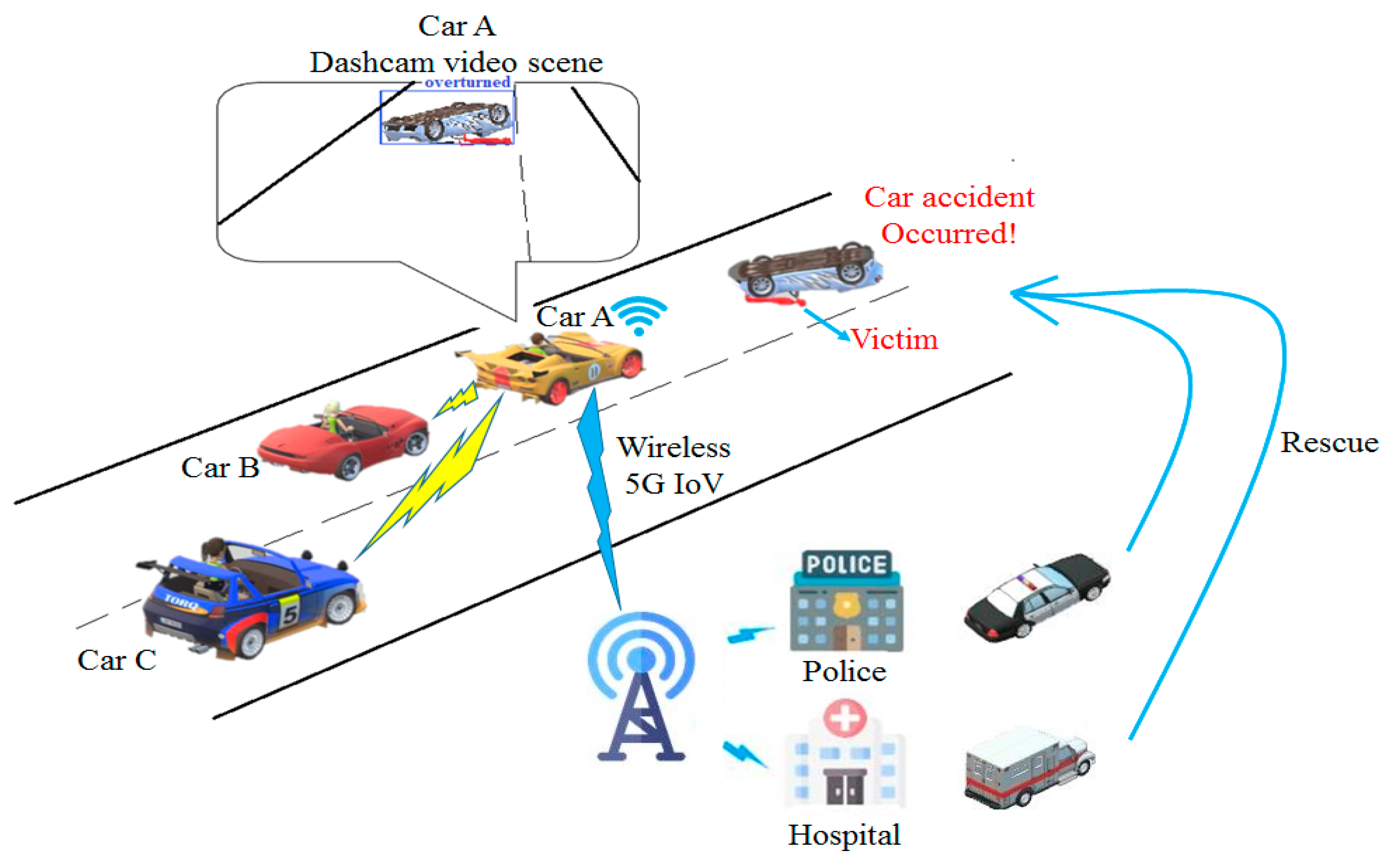
Once a large enough data volume is achieved in the future, the model could even be used to further classify accidents into single-vehicle collisions, rear-end collisions, etc. Moreover, before an accident occurs, some cars may skid or tilt unnaturally. If the detection model can be further developed with these factors in mind, it would have a better predictive ability of accidents before they occur. The accident detection and classification model proposed in this study was developed around the YOLOv3 algorithm. In the future, it is expected that the hardware used in this study can be integrated into the dashcams of self-driving cars. Yet, accident detection is only the first half of the overall scope of application. Generally speaking, in an accident, every aspect is connected-from the moment it happens, to the transmission of information, and to the arrival of rescue teams. The second half will require information connection using 5G IoV, which covers the allocation of 5G resources, and the timeliness and accuracy of information packages. Subsequently, the methods for handling information must be able to minimize the delays that could occur in every aspect, to shorten overall delay and achieve the expectations of this study; that is, reducing delays in receiving medical attention. At present, artificial intelligence (AI) technology is being developed around the world, and communication methods are gradually improving every day. As we usher in the upcoming 5G communication era, the combination of AI and 5G communication is indeed an important development trend. Self-driving car systems should also emphasize driver safety. Therefore, conducting further in-depth research in this aspect would allow us to make contributions in this field.