Robust Filtering for Discrete-Time Linear Parameter-Varying Descriptor Systems

Abstract

This paper deals with robust state estimation for discrete-time, linear parameter varying (LPV) descriptor systems. It is assumed that all the system state-space matrices are affine functions of the uncertain parameters and both the parameters and their variations are bounded functions of time with known minimum and maximum values. First, necessary and sufficient conditions are proposed for admissibility and bounded realness for discrete linear time-varying (DLTV) descriptor systems. Next, two convex optimisation based methods are proposed for designing admissible stationary linear descriptor filters for LPV descriptor systems which ensure a prescribed upper bound on the ${\ell }_2$-induced gain from the noise signal to the estimation error regardless of model uncertainties. The proposed filter design results were based on parameter-dependent generalised Lyapunov functions, and full-order, augmented-order and reduced-order filters were considered. Numerical examples are presented to show the effectiveness of the proposed filtering scheme. In particular, the proposed approach was used to estimate the state variables of a controlled horizontal 2-DOF robotic manipulator based on noisy measurements.

1. Introduction

Nowadays, with the growing use of modern technologies, the dynamics of engineering systems are becoming more complex, and it is of interest to consider more general mathematical representations to cope with advanced real-life systems. In this scenario, descriptor state-space models have attracted the attention of control practitioners, since dynamical and algebraic equations can be embedded into the state-space framework, allowing one to naturally represent more complex systems, such as the ones consisting of subsystems in an interconnected network; see [1,2] and references therein.

Since state estimation is an important issue in analysis, control, monitoring and fault detection of dynamical processes, the problem of state estimation/filtering for descriptor systems has been attracting the attention of researchers in the control community. In the context of ${\mathcal{H}}_{\infty }$ filtering, the design of filters for uncertainty-free, continuous, linear, time-invariant descriptor systems has been addressed in several works (see, e.g., [3,4,5] and references therein), whereas the case of uncertain systems with either norm-bounded or polytopic uncertainties has been studied in, for instance, references [6,7,8] under the assumption that the matrix coefficient E of the state time-derivative is uncertainty-free. On the other hand, the discrete-time counterpart has been the focus of several works. For instance, a method of ${\mathcal{H}}_{\infty }$ filter design for uncertainty-free descriptor systems was proposed in [4] and the problem of robust ${\mathcal{H}}_{\infty }$ filtering was addressed in [9,10,11,12] considering either norm-bounded or polytopic parameter uncertainties.

A common feature of the referred to above works is that they have considered an uncertainty-free matrix E. Recently, a method has been proposed in [13] to design a robust ${\mathcal{H}}_{\infty }$ filter for continuous-time linear descriptor systems with the state time-derivative matrix coefficient E subject to norm-bounded parameter uncertainties. However, it is not possible to extend the result in [13] to discrete-time descriptor systems with all the state-space model matrices (including the E matrix) subject to time-varying uncertain parameters whose values and variations are limited to known intervals. To the authors’ knowledge, the problem of robust ${\mathcal{H}}_{\infty }$ filtering for the latter class of systems has not yet been addressed in specialised literature and it will be investigated in this paper. A motivation for this study is the fact that this class of systems appears in many applications and the problem of state estimation for such systems is of relevance. Specifically, the above referred to descriptor systems can be found in several areas, such as economics and population dynamics—for instance, the singular Leontief dynamic model of a multi-sector economy and the Leslie population model with uncertain parameters; see, e.g., [14,15] and references therein. These models also appear when discretising continuous time-varying descriptor systems arising in power system networks whose circuit elements (e.g., transmission lines and load impedances) may vary within known intervals (see, e.g., [16]) and in mechanical systems, such as robotic manipulators [17], dynamic models of parallel robots [18,19] and uncertain two-mass systems with flexible shafts [20]. However, despite the practical interest, few references deal with control and estimation problems related to LPV discrete-time descriptor systems—see [21] which proposed a gain scheduled approach to the admissibilisation of LPV descriptor systems.

This paper addresses the design of robust ${\mathcal{H}}_{\infty }$ filters for discrete-time linear descriptor systems subject to bounded, time-varying, uncertain parameters whose values are limited to known intervals. In contrast with existing works, uncertain parameters can appear affinely in all the matrices of the system state-space model, including in the one-step-ahead state matrix E, and it is also considered that their variations are constrained to given intervals. The focus of this paper is on developing linear matrix inequality (LMI) based methods to design filters for the latter class of systems which ensure the admissibility (i.e., regularity, causality and exponential stability) of the descriptor estimation error system and a prescribed or optimised upper bound on the ${\ell }_2$-induced gain from the noise signal to the estimation error, irrespective of the uncertain parameters. The main contributions of this paper are as follows:

• Sufficient and a necessary conditions for admissibility and bounded realness for discrete linear time-varying (DLTV) descriptor systems.
• A new dilated bounded real lemma based on the inclusion of slack variables for discrete, linear, parameter-dependent descriptor systems which is tailored for filter design when the descriptor system E matrix is subject to polytopic-type parameter uncertainties.
• Two LMI methods based on novel, parameter-dependent generalised Lyapunov functions to design full-order, augmented-order and reduced order robust ${\mathcal{H}}_{\infty }$ filters for discrete-time linear descriptor systems with uncertain parameters in all the state-space matrices. One of the methods employs a Lyapunov matrix function which depends affinely on the uncertain parameters, whereas for the other one a quadratic parameter-dependence is considered.
• The proposed filtering methods permit one to incorporate in the filter design prior information on known bounds on the variation of the uncertain parameters, which allows one to achieve improved performance when such information is available.

This paper is organised as follows. Section 2 introduces the class of descriptor systems and the admissible filters considered in this paper, and presents the formulation of the robust ${\mathcal{H}}_{\infty }$ filtering problem to be tackled. Section 3 develops conditions for joint admissibility and bounded realness for discrete linear time-varying descriptor systems and results on robust ${\mathcal{H}}_{\infty }$ performance analysis for discrete-time, linear, parameter-dependent descriptor systems. Two design methods of robust ${\mathcal{H}}_{\infty }$ filters are proposed in Section 4 and numerical examples are provided in Section 5 to show the effectiveness of the proposed filtering methods, including a more realistic example which consists of estimating state variables of a controlled horizontal 2-DOF robotic manipulator based on noisy measurements. Section 6 provides some concluding remarks.

Notation.   ${\mathbb{Z}}_i$ is the set of integers equal to or larger than i; $\mathbb{C}$ is the set of complex numbers; ${\mathbb{R}}^{+}$ is the set of positive real numbers; ${\mathbb{R}}^n$ is the n-dimensional Euclidean space; ${\mathbb{R}}^{m\times n}$ is the set of $m\times n$ real matrices; $I_n$ is the $n\times n$ identity matrix; $0_n$ and $0_{m\times n}$ are the $n\times n$ and $m\times n$ matrices of zeros, respectively; and $\mathrm{diag}\{\cdots \}$ stands for a block-diagonal matrix. For a real matrix S, $S^T$ denotes its transpose, $He\left\{S\right\}$ stands for $S+S^T$, $\mathrm{rank}\left\{S\right\}$ is the rank of S and $S>0$ means that S is symmetric and positive-definite. For a symmetric block matrix, the symbol $\star$ denotes the transpose of the blocks outside the main diagonal block. ${\ell }_2$ denotes the space of square summable vector sequences over $[0,\infty )$ with norm ${\parallel ·\parallel }_2$. For a given convex bounded polyhedral domain $\mathcal{X}$, $\mathcal{V}\left(\mathcal{X}\right)$ denotes the set of all the vertices of $\mathcal{X}$.

2. Problem Formulation

Consider the following uncertain discrete-time descriptor system:

$$\left\{\begin{array}{cc}\hfill E\left(\theta \right(k\left)\right)x(k+1)& =A\left(\theta \right(k\left)\right)x\left(k\right)+B\left(\theta \right(k\left)\right)w\left(k\right),\hfill \\ \hfill E\left(\theta \right(0\left)\right)x\left(0\right)& =E\left(\theta \left(0\right)\right)x_0,\hfill \\ \hfill y\left(k\right)& =C_y\left(\theta \left(k\right)\right)x\left(k\right)+D_y\left(\theta \left(k\right)\right)w\left(k\right),\hfill \\ \hfill s\left(k\right)& =C_s\left(\theta \left(k\right)\right)x\left(k\right)+D_s\left(\theta \left(k\right)\right)w\left(k\right),\hfill \end{array}\right.$$

(1)

where $x\left(k\right)\in {\mathbb{R}}^n$ is the state, $w\left(k\right)\in {\mathbb{R}}^{n_w}$ is the disturbance input signal which is assumed to belong to ${\ell }_2$, $y\left(k\right)\in {\mathbb{R}}^{n_y}$ is the measurement, $s\in {\mathbb{R}}^{n_s}$ is the signal to be estimated, $x_0\in {\mathbb{R}}^n$ is the initial state and $\theta \left(k\right)\in {\mathbb{R}}^p$ is a vector of time-varying uncertain parameters. The matrices $E\left(\theta \left(k\right)\right)\in {\mathbb{R}}^{n\times n}$, $A\left(\theta \left(k\right)\right)\in {\mathbb{R}}^{n\times n}$, $B\left(\theta \left(k\right)\right)\in {\mathbb{R}}^{n\times n_w}$, $C_y\left(\theta \left(k\right)\right)\in {\mathbb{R}}^{n_y\times n}$, $D_y\left(\theta \left(k\right)\right)\in {\mathbb{R}}^{n_y\times n_w}$, $C_s\left(\theta \left(k\right)\right)\in {\mathbb{R}}^{n_s\times n}$ and $D_s\left(\theta \left(k\right)\right)\in {\mathbb{R}}^{n_s\times n_w}$ are bounded affine functions of $\theta \left(k\right)$, where $E\left(\theta \right(k\left)\right)$ is allowed to be singular. Due to the fact that the filtering methods to be developed in this paper require system (1) to be regular (see Definition 1 hereafter), it is assumed that $\mathrm{rank}\left\{E\right(\theta \left(k\right)\}=r\le n$ for all admissible $\theta \left(k\right)$. The motivation for this assumption is the fact that for DLTV descriptor systems, oscillatory changes in the rank of the matrix $E\left(k\right)$ cause the system to be non-regular [22]. More specifically, if $\mathrm{rank}\left\{E\right(k\left)\right\}>\mathrm{rank}\left\{E\right(k-1\left)\right\}$ for some integer $k\ge 1$ then the number of algebraic state variables at the instant k becomes larger than the number of algebraic equalities, which implies that either it does not exist a solution for the algebraic state variables at the instant k or there exist several solutions, and thus this system is non-regular. Let ${\theta }_i\left(k\right)\in \mathbb{R}$ be the i-th element of $\theta \left(k\right)$, i.e.,

$$\theta \left(k\right):={\left[\begin{array}{ccc}{\theta }_1\left(k\right)& \cdots & {\theta }_p\left(k\right)\end{array}\right]}^T,$$

and

$$\Delta {\theta }_i\left(k\right):={\theta }_i\left(k\right)-{\theta }_i(k-1)$$

be its backward variation. In this paper, it is assumed that ${\theta }_i\left(k\right)$ and $\Delta {\theta }_i\left(k\right)$, for $i=1,\dots ,p$, are bounded functions of time with known minimum and maximum values. Furthermore, define

$$\Delta \theta \left(k\right):={\left[\begin{array}{ccc}\Delta {\theta }_1\left(k\right)& \cdots & \Delta {\theta }_p\left(k\right)\end{array}\right]}^T=\theta \left(k\right)-\theta (k-1),$$

and let ${\mathcal{X}}_0$ and $\mathcal{X}$ be polytopic sets representing the admissible values of $\theta$ and $(\theta ,\Delta \theta )$, respectively. Moreover, assume that $\mathcal{X}$ is a consistent polytope, as defined in [23], in the sense that if $\left(\theta \right(k),\Delta \theta (k\left)\right)\in \mathcal{X}$, then $\theta (k-1)=\theta \left(k\right)-\Delta \theta \left(k\right)$ belongs to ${\mathcal{X}}_0$. Notice that $\Delta \theta =0$ is an admissible value of $\Delta \theta \left(k\right)$. It is well known that the analysis of descriptor systems is more involved when compared to standard dynamical systems due to the fact that the existence and uniqueness of solution as well as the system causality have to be ascertained. To handle these issues, the following definitions which have been borrowed from [24] (and [25] in the case of exponential stability) will be considered throughout this paper.

Definition 1.

[24,25]  Consider the system in (1). Then:

1. 

 The system is said to be regular if for any consistent $x_0\in {\mathbb{R}}^n$ and $w\left(k\right)\in {\mathbb{R}}^{n_w}$, there exists a solution $x\left(k\right)$ for all $k\in {\mathbb{Z}}_0$ and it is unique.

2. 

 The system is said to be causal if it is regular and the solution $x\left(k\right)$, for any consistent $x_0\in {\mathbb{R}}^n$ and $w\left(k\right)\in {\mathbb{R}}^{n_w}$, is a function of $x_0$ and $w\left(0\right),\dots ,w\left(k\right)$, for all $k\in {\mathbb{Z}}_0$.

3. 

 The system is said to be exponentially stable if it is regular and for any consistent $x_0\in {\mathbb{R}}^n$ and $w\left(k\right)\equiv 0$ there exist real scalars $\alpha >0$ and $\beta \in (0,1)$ such that

$$\parallel x\left(k\right)\parallel \le \alpha {\beta }^k\parallel x_0\parallel ,\forall k\in {\mathbb{Z}}_1.$$

4. 

 The system is said to be admissible if it is causal and exponentially stable.

Remark 1.

The concepts of regularity, causality and exponential stability in Definition 1 are the conceptual definitions of those concepts and they apply to linear and nonlinear (time-invariant and time-varying) descriptor systems. Note that the definitions of regularity, causality and exponential stability used in many works dealing with linear discrete time-invariant descriptor systems are in terms of structural properties of the pair $(E,A)$ (see, e.g., [3,11,12]), and they are in fact criteria for those properties to hold.

In Appendix A.1 we recall a result from [24] which establishes a necessary and sufficient condition of causality for DLTV descriptor systems. From Definition 1, the notion of robust admissibility to be considered from now on will be introduced.

Definition 2.

System (1) is said to be robustly admissible if it is admissible for all $(\theta ,\Delta \theta )\in \mathcal{X}$.

The problem of concern in this paper consists of designing a stationary filter to obtain an estimate $s_f\left(k\right)$ of $s\left(k\right)$ which ensures a uniformly small (in the ${\ell }_2$-norm sense) estimation error $e\left(k\right)$ for any $w\in {\ell }_2$ and $\left(\theta \right(k),\Delta \theta (k\left)\right)\in \mathcal{X}$, where

$$e\left(k\right):=s\left(k\right)-s_f\left(k\right).$$

(2)

To this end, consider the following filter:

$$\left\{\begin{array}{cc}\hfill E_f{x}_f(k+1)& =A_f{x}_f\left(k\right)+B_{f}y\left(k\right),E_f{x}_f\left(0\right)=E_f{x}_{f0},\hfill \\ \hfill s_f\left(k\right)& =C_f{x}_f\left(k\right)+D_{f}y\left(k\right),\hfill \end{array}\right.$$

(3)

where $x_f\left(k\right)\in {\mathbb{R}}^n$ is the filter state, $x_{f0}\in {\mathbb{R}}^n$ is the initial filter state (assumed to be consistent), $E_f\in {\mathbb{R}}^{n\times n}$, $A_f\in {\mathbb{R}}^{n\times n}$, $B_f\in {\mathbb{R}}^{n\times n_y}$, $C_f\in {\mathbb{R}}^{n_s\times n}$ and $D_f\in {\mathbb{R}}^{n_s\times n_y}$ are constant matrices to be determined. Moreover, it is assumed that $\mathrm{rank}\left\{E_f\right\}=r_f$, for a given $r_f\le n$, and $E_f$ is as follows:

$$E_f=\left[\begin{array}{cc}{I}_{r_f}& 0\\ 0& 0_{n-r_f}\end{array}\right].$$

(4)

Observe that the filter is allowed to be a descriptor system and the rank $r_f$ of the filter matrix $E_f$ coincides with the degree of the filter characteristic polynomial, i.e., $\mathrm{deg}\left\{\det (z{E}_f-A_f)\right\}$, $\forall z\in \mathbb{C}$. The following structures for the matrix $E_f$ will be considered depending on the choice of $r_f$, which is also the number of dynamic state variables of the filter:

I) 

Full-order filter: $r_f=r$,  with

$$E_f=\left[\begin{array}{cc}{I}_r& 0\\ 0& 0_{n-r}\end{array}\right].$$

II) 

Augmented-order filter: $r_f=n$,  with

$$E_f=I_n.$$

III) 

Reduced-order filter: $r_f<r$,  with

$$E_f=\left[\begin{array}{cc}{I}_{r_f}& 0\\ 0& 0_{n-r_f}\end{array}\right].$$

It should be noted that, as in the context of standard state-space models, the relation between the number of dynamic state variables of the filter (i.e., $r_f$) and of the descriptor system (i.e., r) was chosen to characterise the notions of full-order, augmented-order and reduced-order filters. For instance, a full-order filter is the one whose number of dynamic state variables is the same as for the system. Hereafter, the rank, $r_f$, of the filter matrix $E_f$ will be referred to as the filter order. In view of (1) and (3), the estimation error dynamics can be described by the following descriptor system, which will be referred to as the estimation error system:

$$\{\begin{array}{cc}\hfill E_a\left(\theta \left(k\right)\right)\xi (k+1)& =A_a\left(\theta \left(k\right)\right)\xi \left(k\right)+B_a\left(\theta \left(k\right)\right)w\left(k\right),\hfill \\ \hfill E_a\left(\theta \left(0\right)\right)\xi \left(0\right)& ={\left[\begin{array}{cc}{\left(E\left(\theta \left(0\right)\right)x_0\right)}^T& {\left(E_f{x}_{f0}\right)}^T\end{array}\right]}^T,\hfill \\ \hfill e\left(k\right)& =C_a\left(\theta \left(k\right)\right)\xi \left(k\right)+D_a\left(\theta \left(k\right)\right)w\left(k\right),\hfill \end{array}$$

(5)

where

$$\begin{array}{cc}\hfill \xi \left(k\right)& =\left[\begin{array}{c}x\left(k\right)\\ x_f\left(k\right)\end{array}\right],E_a\left(\theta \left(k\right)\right)=\left[\begin{array}{cc}E\left(\theta \right(k\left)\right)& 0\\ 0& E_f\end{array}\right],\hfill \\ \hfill A_a\left(\theta \left(k\right)\right)& =\left[\begin{array}{cc}A\left(\theta \right(k\left)\right)& 0\\ B_f{C}_y\left(\theta \left(k\right)\right)& A_f\end{array}\right],\hfill \\ \hfill B_a\left(\theta \left(k\right)\right)& =\left[\begin{array}{c}B\left(\theta \right(k\left)\right)\\ B_f{D}_y\left(\theta \left(k\right)\right)\end{array}\right],\hfill \\ \hfill C_a\left(\theta \left(k\right)\right)& =\left[\begin{array}{cc}{C}_s\left(\theta \left(k\right)\right)-D_f{C}_y\left(\theta \left(k\right)\right)& -C_f\end{array}\right],\hfill \\ \hfill D_a\left(\theta \left(k\right)\right)& =D_s\left(\theta \left(k\right)\right)-D_f{D}_y\left(\theta \left(k\right)\right).\hfill \\ \hfill & \hfill \end{array}$$

(6)

Observe that $\mathrm{rank}\left\{E_a\left(\theta \right)\right\}=r+r_f\le 2n$ for all $\theta \in {\mathcal{X}}_0$. In the above context, the filtering problem to be addressed in this paper consists of finding a filter given by (3) and (4) (either full-order, augmented-order or reduced-order), guaranteeing the robust admissibility of the estimation error system (5) while ensuring a prescribed or optimised upper bound on the ${\ell }_2$-induced gain from w to e of the estimation error system (5), which is defined as follows:

$$\parallel {\mathcal{G}}_{we}{\parallel }_{\infty }=\underset{w\in {\ell }_2}{sup}\left\{\frac{{\parallel e\left(k\right)\parallel }_2}{{\parallel w\left(k\right)\parallel }_2}:w\left(k\right)\not\equiv 0,E_a\left(\theta \left(0\right)\right)\xi \left(0\right)=0\right\}.$$

3. ${\mathcal{H}}_{\infty }$ Performance for Descriptor Systems

This section presents results on robust ${\mathcal{H}}_{\infty }$ performance analysis of descriptor systems. These results will be used for deriving the robust ${\mathcal{H}}_{\infty }$ filters of this paper. Firstly, we address the issues of admissibility and bounded realness of DLTV descriptor systems, which will be instrumental to obtain the robust ${\mathcal{H}}_{\infty }$ performance analysis results presented in the following. To this end, consider the DLTV descriptor system:

$$\left\{\begin{array}{cc}\hfill E\left(k\right)x(k+1)& =A\left(k\right)x\left(k\right)+B\left(k\right)w\left(k\right),\hfill \\ \hfill E\left(0\right)x\left(0\right)& =E\left(0\right)x_0,\hfill \\ \hfill s\left(k\right)& =C\left(k\right)x\left(k\right)+D\left(k\right)w\left(k\right),\hfill \end{array}\right.$$

(7)

where $x\left(k\right)\in {\mathbb{R}}^n$ is the state; $w\left(k\right)\in {\mathbb{R}}^{n_w}$ is a disturbance input belonging to ${\ell }_2$; $s\left(k\right)\in {\mathbb{R}}^{n_s}$ is the performance output; $x_0\in {\mathbb{R}}^n$ is the initial state; and $A\left(k\right)\in {\mathbb{R}}^{n\times n}$, $B\left(k\right)\in {\mathbb{R}}^{n\times n_w}$, $C\left(k\right)\in {\mathbb{R}}^{n_s\times n}$, $D\left(k\right)\in {\mathbb{R}}^{n_s\times n_w}$ and $E\left(k\right)\in {\mathbb{R}}^{n\times n}$ are bounded time-varying matrices, subject to the assumption $\mathrm{rank}\left\{E\left(k\right)\right\}=r\le n$ for all $k\in {\mathbb{Z}}_0$; the reader is referred to Section 2 for the motivation of the latter assumption. The following lemma proposed in [24] provides a necessary and sufficient condition for the admissibility of system (7).

Lemma 1.

[24] Consider the descriptor system of (7) with $w\left(k\right)\equiv 0$. Let $S\left(k\right)\in {\mathbb{R}}^{n\times (n-r)}$ be a bounded time-varying matrix such that $E^T\left(k\right)S\left(k\right)=0$, with $\mathrm{rank}\left\{S\right(k\left)\right\}=n-r$ for all $k\in {\mathbb{Z}}_0$. Then, system (7) is admissible if and only if there exist bounded time-varying matrices $Q\left(k\right)$ and $X(k-1)>0,\forall k\in {\mathbb{Z}}_0$, satisfying the following matrix inequality:

$$A^T\left(k\right)X\left(k\right)A\left(k\right)+\mathrm{He}\left\{A^T\left(k\right)S\left(k\right)Q\left(k\right)\right\}-E^T(k-1)X(k-1)E(k-1)<0,\forall k\in {\mathbb{Z}}_0,$$

(8)

with $E(-1):=E\left(0\right)$.

Note that, inspired by the notion of generalised Lyapunov functions introduced in [26], the function

$$V(x\left(k\right),k):=x^T\left(k\right)E^T(k-1)X(k-1)E(k-1)x\left(k\right)$$

(9)

can be viewed as a generalised Lyapunov function for the unforced system of (7).

The next result, which is based on the authors’ conference paper [27], presents a bounded real lemma for the time-varying descriptor system in (7).

Lemma 2.

Consider the descriptor system in (7) and let $\gamma >0$ be a given scalar and $S\left(k\right)\in {\mathbb{R}}^{n\times (n-r)}$ a bounded time-varying matrix such that $E^T\left(k\right)S\left(k\right)=0$, with $\mathrm{rank}\left\{S\right(k\left)\right\}=n-r$ for all $k\in {\mathbb{Z}}_0$. Then, the following conditions hold:

(i) 

System (7) is admissible and $\parallel {\mathcal{G}}_{ws}{\parallel }_{\infty }<\gamma$ if there exist bounded time-varying matrices $Q\left(k\right)$ and $X(k-1)>0$, $\forall k\in {\mathbb{Z}}_0$, satisfying the following matrix inequality:

$$\left[\begin{array}{ccc}{\mathrm{Y}}_1\left(k\right)& \star & \star \\ {\mathrm{Y}}_2\left(k\right)& B^T\left(k\right)X\left(k\right)B\left(k\right)-\gamma I& \star \\ C\left(k\right)& D\left(k\right)& -\gamma I\end{array}\right]<0,\forall k\in {\mathbb{Z}}_0,$$

(10)

where $E(-1):=E\left(0\right)$ and

$$\begin{array}{cc}\hfill {\mathrm{Y}}_1\left(k\right)& =A^T\left(k\right)X\left(k\right)A\left(k\right)+\mathrm{He}\left\{A^T\left(k\right)S\left(k\right)Q\left(k\right)\right\}-E^T(k-1)X(k-1)E(k-1),\hfill \end{array}$$

(11)

$$\begin{array}{cc}\hfill {\mathrm{Y}}_2\left(k\right)& =B^T\left(k\right)X\left(k\right)A\left(k\right)+B^T\left(k\right)S\left(k\right)Q\left(k\right).\hfill \end{array}$$

(12)

(ii) 

Subject to either the assumption $Ker\left\{E^T\left(k\right)\right\}\subseteq Ker\left\{B^T\left(k\right)\right\}$ for all $k\in {\mathbb{Z}}_0$ or $Ker\left\{E\right(k\left)\right\}\subseteq Ker\left\{C\right(k+1\left)\right\}$ for all $k\in {\mathbb{Z}}_{-1}$, if system (7) is admissible and $\parallel {\mathcal{G}}_{ws}{\parallel }_{\infty }<\gamma$, then there exist bounded time-varying matrices $Q\left(k\right)$ and $X(k-1)>0$, $\forall k\in {\mathbb{Z}}_0$, satisfying the matrix inequality (10).

Proof. 

  See Appendix A.1. □

Lemma 2 presents, for the first time, necessary and sufficient conditions for the solvability of the ${\mathcal{H}}_{\infty }$ performance analysis problem for discrete-time linear descriptor systems with all the state-space model matrices being bounded time-varying functions. The assumption $\mathrm{Ker}\left\{E^T\left(k\right)\right\}\subseteq \mathrm{Ker}\left\{B^T\left(k\right)\right\}$, $\forall k\in {\mathbb{Z}}_0$, which appears in the necessary condition $\left(ii\right)$ of Lemma 2, implies that the system algebraic constraints do not depend on the disturbance $w\left(k\right)$. On the other hand, $\mathrm{Ker}\left\{E\left(k\right)\right\}\subseteq \mathrm{Ker}\left\{C\left(k+1\right)\right\},\forall k\in {\mathbb{Z}}_{-1}$, means that the system performance output $s\left(k\right)$ depends only on the dynamic state variables of the system. In the following a direct extension of Lemma 2 to cope with time-varying parameter-dependent matrices is introduced. Firstly, take the following linear parameter-dependent descriptor system:

$$\left\{\begin{array}{cc}\hfill E\left(\theta \right(k\left)\right)x(k+1)& =A\left(\theta \right(k\left)\right)x\left(k\right)+B\left(\theta \right(k\left)\right)w\left(k\right),\hfill \\ \hfill E\left(\theta \right(0\left)\right)x\left(0\right)& =E\left(\theta \left(0\right)\right)x_0,\hfill \\ \hfill s\left(k\right)& =C_s\left(\theta \left(k\right)\right)x\left(k\right)+D_s\left(\theta \left(k\right)\right)w\left(k\right),\hfill \end{array}\right.$$

(13)

where the matrices and vectors are as defined in Section 2. To ease the notation, the dependence of $\theta \left(k\right)$ and $\Delta \theta \left(k\right)$ on k will be hereafter often omitted.

Lemma 3.

Consider the uncertain descriptor system as in (13). Let ${\mathcal{X}}_0$ and $\mathcal{X}$ be given polytopes of admissible θ and $(\theta ,\Delta \theta )$, respectively, and $\gamma >0$ a given scalar. Assume that there exists a bounded matrix function $S\left(\theta \right)\in {\mathbb{R}}^{n\times (n-r)}$ such that $\mathrm{rank}\left\{S\right(\theta \left)\right\}=n-r$ and $E^T\left(\theta \right)S\left(\theta \right)=0,\forall \theta \in {\mathcal{X}}_0$. Then, system (13) is robustly admissible and $\parallel {\mathcal{G}}_{ws}{\parallel }_{\infty }<\gamma$, for all $(\theta ,\Delta \theta )\in \mathcal{X}$, if any of the following equivalent conditions holds:

(i) 

There exist bounded matrix functions $Q\left(\theta \right)$ and $X\left(\theta \right)>0$, $\forall \theta \in {\mathcal{X}}_0$, with appropriate dimensions satisfying the following matrix inequality:

$$\left[\begin{array}{ccc}{\tilde{\mathrm{Y}}}_1(\theta ,\Delta \theta )& \star & \star \\ {\tilde{\mathrm{Y}}}_2\left(\theta \right)& B^T\left(\theta \right)X\left(\theta \right)B\left(\theta \right)-\gamma I& \star \\ C_s\left(\theta \right)& D_s\left(\theta \right)& -\gamma I\end{array}\right]<0,\forall (\theta ,\Delta \theta )\in \mathcal{X},$$

(14)

where

$$\begin{array}{cc}\hfill {\tilde{\mathrm{Y}}}_1(\theta ,\Delta \theta )& =A^T\left(\theta \right)X\left(\theta \right)A\left(\theta \right)+\mathrm{He}\left\{A^T\left(\theta \right)S\left(\theta \right)Q\left(\theta \right)\right\}-E^T(\theta -\Delta \theta )X(\theta -\Delta \theta )E(\theta -\Delta \theta ),\hfill \end{array}$$

(15)

$$\begin{array}{cc}\hfill {\tilde{\mathrm{Y}}}_2\left(\theta \right)& =B^T\left(\theta \right)X\left(\theta \right)A\left(\theta \right)+B^T\left(\theta \right)S\left(\theta \right)Q\left(\theta \right).\hfill \end{array}$$

(16)

(ii) 

There exist bounded matrix functions $F\left(\theta \right)$, $G\left(\theta \right)$, $H\left(\theta \right)$, $R\left(\theta \right)$ and $P\left(\theta \right)>0,\forall \theta \in {\mathcal{X}}_0$, with appropriate dimensions satisfying the following matrix inequality:

$$\left[\begin{array}{ccccc}{\mathsf{\Omega }}_1(\theta ,\Delta \theta )& \star & \star & \star & \star \\ B^T\left(\theta \right)F^T\left(\theta \right)& -\gamma I& \star & \star & \star \\ {\mathsf{\Omega }}_2\left(\theta \right)& G\left(\theta \right)B\left(\theta \right)& {\mathsf{\Omega }}_3\left(\theta \right)& \star & \star \\ -H^T\left(\theta \right)& 0& 0& -P(\theta -\Delta \theta )& \star \\ C_s\left(\theta \right)& D_s\left(\theta \right)& 0& 0& -\gamma I\end{array}\right]<0,\forall (\theta ,\Delta \theta )\in \mathcal{X},$$

(17)

where

$$\begin{array}{cc}\hfill {\mathsf{\Omega }}_1(\theta ,\Delta \theta )& =\mathrm{He}\left\{F\right(\theta \left)A\right(\theta )+H(\theta \left)E\right(\theta -\Delta \theta \left)\right\},\hfill \end{array}$$

(18)

$$\begin{array}{cc}\hfill {\mathsf{\Omega }}_2\left(\theta \right)& =S\left(\theta \right)R\left(\theta \right)+G\left(\theta \right)A\left(\theta \right)-F^T\left(\theta \right),\hfill \end{array}$$

(19)

$$\begin{array}{cc}\hfill {\mathsf{\Omega }}_3\left(\theta \right)& =P\left(\theta \right)-G\left(\theta \right)-G^T\left(\theta \right).\hfill \\ \hfill \end{array}$$

(20)

Proof.  

(i) 

 It will be shown that statement $\left(i\right)$ of Lemma 3 is equivalent to Lemma 2 $\left(i\right)$. To this end, noting that $\theta \left(k\right)-\Delta \theta \left(k\right)=\theta (k-1)$ and considering that (14) holds for any $\theta \left(k\right)\in {\mathcal{X}}_0$ and $\left(\theta \right(k),\Delta \theta (k\left)\right)\in \mathcal{X}$, then statement $\left(i\right)$ of Lemma 3 coincides with Lemma 2 $\left(i\right)$ with $A\left(k\right)=A\left(\theta \left(k\right)\right),B\left(k\right)=B\left(\theta \left(k\right)\right),C\left(k\right)=C_s\left(\theta \left(k\right)\right),D\left(k\right)=D_s\left(\theta \left(k\right)\right),E\left(k\right)=E\left(\theta \left(k\right)\right)$, $S\left(k\right)=S\left(\theta \right(k\left)\right)$, $X\left(k\right)=X\left(\theta \right(k\left)\right)$ and $Q\left(k\right)=Q\left(\theta \right(k\left)\right)$.

(i) 

⇒ (ii) Suppose there exist bounded matrix functions $Q\left(\theta \right)$ and $X\left(\theta \right)>0,\forall \theta \in {\mathcal{X}}_0$, satisfying (14). Applying Schur complements, it follows that (14) is equivalent to

$$\left[\begin{array}{ccccc}{Y}_1\left(\theta \right)& \star & \star & \star & \star \\ Y_2\left(\theta \right)& -\gamma I& \star & \star & \star \\ X\left(\theta \right)A\left(\theta \right)& X\left(\theta \right)B\left(\theta \right)& -X\left(\theta \right)& \star & \star \\ X\left({\theta }_{-}\right)E\left({\theta }_{-}\right)& 0& 0& -X\left({\theta }_{-}\right)& \star \\ C_s\left(\theta \right)& D_s\left(\theta \right)& 0& 0& -\gamma I\end{array}\right]<0,$$

(21)

where

$$\begin{array}{cc}\hfill & E\left({\theta }_{-}\right):=E(\theta -\Delta \theta ),X\left({\theta }_{-}\right):=X(\theta -\Delta \theta ),\hfill \\ \hfill & Y_1\left(\theta \right)=\mathrm{He}\left\{A^T\left(\theta \right)S\left(\theta \right)Q\left(\theta \right)\right\}-E^T\left({\theta }_{-}\right)X\left({\theta }_{-}\right)E\left({\theta }_{-}\right),\hfill \\ \hfill & Y_2\left(\theta \right)=B^T\left(\theta \right)S\left(\theta \right)Q\left(\theta \right).\hfill \\ \hfill & \hfill \end{array}$$

It can then be readily verified that (21) ensures that (17) is satisfied with $F^T\left(\theta \right)=S\left(\theta \right)Q\left(\theta \right),G\left(\theta \right)=P\left(\theta \right)=X\left(\theta \right)$, $H\left(\theta \right)=-E^T(\theta -\Delta \theta )X(\theta -\Delta \theta )$ and $R\left(\theta \right)=Q\left(\theta \right)$.

(ii) 

⇒ (i) Suppose that statement $\left(ii\right)$ of Lemma 3 is fulfilled. Pre- and post-multiplying (17) by

$$\left[\begin{array}{ccccc}{I}_n& 0_{n\times n_w}& A^T\left(\theta \right)& E^T(\theta -\Delta \theta )& 0_{n\times n_s}\\ 0_{n_w\times n}& I_{n_w}& B^T\left(\theta \right)& 0_{n_w\times n}& 0_{n_w\times n_s}\\ 0_{n_s\times n}& 0_{n_s\times n_w}& 0_{n_s\times n}& 0_{n_s\times n}& I_{n_s}\end{array}\right]$$

and its transpose, respectively, leads to the inequality (14) with $Q\left(\theta \right)$ and $X\left(\theta \right)$ replaced by $R\left(\theta \right)$ and $P\left(\theta \right)$, respectively. This implies that statement $\left(i\right)$ of Lemma 3 is satisfied with $Q\left(\theta \right)=R\left(\theta \right)$ and $X\left(\theta \right)=P\left(\theta \right)$. □

For robust filter design, it turns out that condition (17) of Lemma 3 is potentially less conservative than that in (14). This follows from the fact that, due to the presence of the auxiliary matrices $F\left(\theta \right)$, $G\left(\theta \right)$ and $H\left(\theta \right)$ in (17), it is not necessary to parameterise the filter matrices in terms of the Lyapunov matrix $P\left(\theta \right)$, as is shown in the next section.

4. Robust ${\mathcal{H}}_{\infty }$ Filter Design

This section deals with the robust ${\mathcal{H}}_{\infty }$ filtering problem for the uncertain descriptor system (1). In particular, a filter as in (3) is designed such that the estimation error system (5) satisfies Lemma 3 $\left(ii\right)$. The straightforward application of this lemma leads to a nonlinear matrix inequality, namely, there exist matrices $A_f,B_f,C_f$ and $D_f$, and matrix functions $F\left(\theta \right),G\left(\theta \right),H\left(\theta \right),R\left(\theta \right)$ and $P\left(\theta \right)>0,\forall \theta \in {\mathcal{X}}_0,$ satisfying:

$$\left[\begin{array}{ccccc}{\widehat{\mathsf{\Omega }}}_1(\theta ,\Delta \theta )& \star & \star & \star & \star \\ B_a^T\left(\theta \right)F^T\left(\theta \right)& -\gamma I& \star & \star & \star \\ {\widehat{\mathsf{\Omega }}}_2\left(\theta \right)& G\left(\theta \right)B_a\left(\theta \right)& {\widehat{\mathsf{\Omega }}}_3\left(\theta \right)& \star & \star \\ -H^T\left(\theta \right)& 0& 0& -P(\theta -\Delta \theta )& \star \\ C_a\left(\theta \right)& D_a\left(\theta \right)& 0& 0& -\gamma I\end{array}\right]<0,\forall (\theta ,\Delta \theta )\in \mathcal{X},$$

(22)

where

$$\left\{\begin{array}{c}{\widehat{\mathsf{\Omega }}}_1(\theta ,\Delta \theta )=\mathrm{He}\left\{F\left(\theta \right)A_a\left(\theta \right)+H\left(\theta \right)E_a(\theta -\Delta \theta )\right\},\hfill \\ {\widehat{\mathsf{\Omega }}}_2\left(\theta \right)=S_a\left(\theta \right)R\left(\theta \right)+G\left(\theta \right)A_a\left(\theta \right)-F^T\left(\theta \right),\hfill \\ {\widehat{\mathsf{\Omega }}}_3\left(\theta \right)=P\left(\theta \right)-G\left(\theta \right)-G^T\left(\theta \right).\hfill \end{array}\right.$$

(23)

and $S_a\left(\theta \right)\in {\mathbb{R}}^{2n\times (2n-r-r_f)}$ is a bounded matrix function of $\theta$ such that $\mathrm{rank}\left\{S_a\left(\theta \right)\right\}=2n-r-r_f$ and $E_a^T\left(\theta \right)S_a\left(\theta \right)=0$ for all $\theta \in {\mathcal{X}}_0$. Observe that in view of the structure of the matrix $E_a\left(\theta \right)$, a suitable matrix $S_a\left(\theta \right)$ when $r_f<n$ is as follows:

$$S_a\left(\theta \right)=\left[\begin{array}{cc}S\left(\theta \right)& 0_{n\times (n-r_f)}\\ 0_{r_f\times (n-r)}& 0_{r_f\times (n-r_f)}\\ 0_{(n-r_f)\times (n-r)}& I_{n-r_f}\end{array}\right],$$

(24)

where $S\left(\theta \right)\in {\mathbb{R}}^{n\times (n-r)}$ is a bounded matrix function of $\theta$ such that $\mathrm{rank}\left\{S\right(\theta \left)\right\}=n-r$ and $E^T\left(\theta \right)S\left(\theta \right)=0$ for all $\theta \in {\mathcal{X}}_0$. On the other hand, in the case of an augmented-order filter design (i.e., $E_f=I_n$), the matrix $S_a\left(\theta \right)$ reduces to the following:

$$S_a\left(\theta \right)={\left[\begin{array}{cc}{S}^T\left(\theta \right)& 0_{n\times (n-r)}^T\end{array}\right]}^T.$$

(25)

Note that

$$V(x,k)=x^T\left(k\right)E^T\left(\theta (k-1)\right)P\left(\theta (k-1)\right)E\left(\theta (k-1)\right)x\left(k\right),$$

with $P\left(\theta \right)>0,\forall \theta \in {\mathcal{X}}_0$ and satisfying (22) is a generalised Lyapunov function for the estimation error system (5).

Note that (22) is nonlinear with respect to $\theta$ and decision variables (there are products involving affine dependent matrices and between filter matrices and blocks of the matrices $F\left(\theta \right)$ and $G\left(\theta \right)$). Hence, (22) should be satisfied over the entire polytope $\mathcal{X}$ leading to an infinite-dimensional problem, which in general, is very hard to be numerically solved. In order to overcome this difficulty, in the following, we constrain the matrix $S\left(\theta \right)$ to be an affine matrix function of $\theta$, impose some constraints to the matrices $F\left(\theta \right),G\left(\theta \right),H\left(\theta \right)$ and $R\left(\theta \right)$ and propose two relaxation techniques. The following assumption will be hereafter adopted:

Assumption 1.

There exists an affine matrix function $S\left(\theta \right)\in {\mathbb{R}}^{n\times (n-r)}$ such that $\mathrm{rank}\left\{S\right(\theta \left)\right\}=n-r$ and $E^T\left(\theta \right)S\left(\theta \right)=0$, for all $\theta \in {\mathcal{X}}_0$.

Remark 2.

The above assumption is considered in order to derive numerically tractable filter design conditions in terms of a finite number of LMIs later in this paper. It should be pointed out that Assumption 1 does not introduce any conservatism to the filter design methods proposed in the paper. Observe that this assumption may only limit the applicability of the design methods because there may exist descriptor systems with $n\times n$ one-step-ahead state matrix $E\left(\theta \right)$ satisfying $\mathrm{rank}\left\{E\right(\theta \left)\right\}=r<n$, for all admissible parameters θ, which does not satisfy Assumption 1. Note that, following similar arguments as in [28], an affine matrix function $E\left(\theta \right)$ can be described as: $\left(i\right)$ $E\left(\theta \right)$ = $J_{\ell }[I_n+D_{\ell }\left(\theta \right)]$, or $\left(ii\right)$ $E\left(\theta \right)=[I_n+D_r\left(\theta \right)]J_r$, where $J_{\ell }$ and $J_r$ are constant matrices with rank r; and $D_{\ell }$ and $D_r$ are affine matrix functions of θ such that $[I_n+D_{\ell }\left(\theta \right)]$ and $[I_n+D_r\left(\theta \right)]$ are nonsingular matrices. Thus, it follows that Assumption 1 is always satisfied in case $\left(i\right)$ with a constant matrix S, whereas in case $\left(ii\right)$ it may or not be satisfied.

Remark 3.

It should be remarked that in the case wherein the attention is focused on designing an augmented-order filter (i.e, $E_f=I_n$), and (22) holds with a matrix $G\left(\theta \right)$ as follows:

$$G\left(\theta \right)=\left[\begin{array}{cc}{G}_1\left(\theta \right)& G_3\\ G_2\left(\theta \right)& G_4\end{array}\right],G_1\left(\theta \right),G_2\left(\theta \right),G_3,G_4\in {\mathbb{R}}^{n\times n},$$

(26)

where the matrices $G_3$ and $G_4$ are independent of θ, as will be shown in the next lemma, it turns out that, without loss of generality, it can be assumed that $G_3=G_4$.

Lemma 4.

Consider the estimation error system in (5) with $E_f=I_n$ and suppose there exist matrices $A_f$, $B_f$, $C_f$, $D_f$, $F\left(\theta \right)$, $H\left(\theta \right)$, $R\left(\theta \right)$, $P\left(\theta \right)>0,\forall \theta \in {\mathcal{X}}_0$, and $G\left(\theta \right)$ as in (26) such that (22) holds. Then, there exist matrices ${\breve{A}}_f,{\breve{B}}_f,{\breve{C}}_f,{\breve{D}}_f,\breve{F}\left(\theta \right),\breve{H}\left(\theta \right)$, $\breve{R}\left(\theta \right),\breve{P}\left(\theta \right)>0,\forall \theta \in {\mathcal{X}}_0$ and $\breve{G}\left(\theta \right)$ as given below.

$$\breve{G}\left(\theta \right)=\left[\begin{array}{cc}{\breve{G}}_1\left(\theta \right)& {\breve{G}}_3\\ {\breve{G}}_2\left(\theta \right)& {\breve{G}}_3\end{array}\right],{\breve{G}}_1\left(\theta \right),{\breve{G}}_2\left(\theta \right),{\breve{G}}_3\in {\mathbb{R}}^{n\times n},$$

(27)

where ${\breve{G}}_3$ is independent of θ, such that (22) is satisfied with $A_f$, $B_f$, $C_f,D_f,F\left(\theta \right),H\left(\theta \right),R\left(\theta \right),P\left(\theta \right)$ and $G\left(\theta \right)$ replaced by ${\breve{A}}_f,{\breve{B}}_f,{\breve{C}}_f,{\breve{D}}_f,\breve{F}\left(\theta \right),\breve{H}\left(\theta \right)$, $\breve{R}\left(\theta \right),\breve{P}\left(\theta \right)$ and $\breve{G}\left(\theta \right)$, respectively.

Proof. 

See Appendix A.2. □

Next, two computable approaches to the filter design are proposed. For the first relaxation technique, it is considered that the matrices $F\left(\theta \right),G\left(\theta \right),H\left(\theta \right)$ and $R\left(\theta \right)$ are independent of $\theta$, whereas the Lyapunov matrix $P\left(\theta \right)$ is an affine function of $\theta$ as follows:

$$P\left(\theta \right)=P_0+{\theta }_1{P}_1+\cdots +{\theta }_p{P}_p,$$

(28)

where $P_i=P_i^T\in {\mathbb{R}}^{2n\times 2n},i=0,\dots ,p$, are matrices to be determined. Moreover, since in (22) the filter matrices $A_f$ and $B_f$ appear, multiplying simultaneously blocks of the matrices F and G, in order to obtain a filter design in terms of LMIs, structure constraints will be imposed to the matrices F and G leading to the following result.

Theorem 1.

Consider the uncertain descriptor system as in (1) with Assumption 1, and let ${\mathcal{X}}_0$ and $\mathcal{X}$ be given polytopes of admissible θ and $(\theta ,\Delta \theta )$, respectively. A given order $r_f$ of the filter is to be designed, with $r_f\le n$ and $\gamma >0$ a given scalar. Suppose that for given scalars ϵ and μ there exist matrices $\widehat{F}\in {\mathbb{R}}^{2n\times n}$, $\widehat{G}\in {\mathbb{R}}^{2n\times n}$, $H\in {\mathbb{R}}^{2n\times 2n},$  $K\in {\mathbb{R}}^{n\times n}$, ${\Pi }_a\in {\mathbb{R}}^{n\times n}$, ${\Pi }_b\in {\mathbb{R}}^{n\times n_y}$, ${\Pi }_c\in {\mathbb{R}}^{n_s\times n}$, ${\Pi }_d\in {\mathbb{R}}^{n_s\times n_w}$, $R\in {\mathbb{R}}^{(2n-r-r_f)\times 2n}$ and $P_i=P_i^T\in {\mathbb{R}}^{2n\times 2n},i=0,1,\cdots ,p$, satisfying the following LMIs:

$$\begin{array}{cc}\hfill P\left(\theta \right)& >0,\forall \theta \in \mathcal{V}\left({\mathcal{X}}_0\right),\hfill \end{array}$$

(29)

$$\begin{array}{cc}\hfill \left[\begin{array}{ccccc}{\Sigma }_1\left(\theta \right)& \star & \star & \star & \star \\ {\Sigma }_2\left(\theta \right)& -\gamma I& \star & \star & \star \\ {\Sigma }_3\left(\theta \right)& {\Sigma }_4\left(\theta \right)& {\Sigma }_5\left(\theta \right)& \star & \star \\ -H^T& 0& 0& -P(\theta -\Delta \theta )& \star \\ {\Sigma }_6\left(\theta \right)& {\Sigma }_7\left(\theta \right)& 0& 0& -\gamma I\end{array}\right]& <0,\forall (\theta ,\Delta \theta )\in \mathcal{V}\left(\mathcal{X}\right),\hfill \end{array}$$

(30)

where $P\left(\theta \right)$ is given in (28) and

$$\begin{array}{cc}\hfill & {\Sigma }_1\left(\theta \right)=\mathrm{He}\left\{\left[\begin{array}{cc}\widehat{F}A\left(\theta \right)+{\mathcal{I}}_f{\Pi }_b{C}_y\left(\theta \right)& {\mathcal{I}}_f{\Pi }_a\end{array}\right]+H{E}_a(\theta -\Delta \theta )\right\},\hfill \\ \hfill & {\Sigma }_2\left(\theta \right)=B^T\left(\theta \right){\widehat{F}}^T+D_y^T\left(\theta \right){\Pi }_b^T{\mathcal{I}}_f^T,\hfill \\ \hfill & {\Sigma }_3\left(\theta \right)=S_a\left(\theta \right)R+\left[\begin{array}{cc}\widehat{G}A\left(\theta \right)+{\mathcal{I}}_g{\Pi }_b{C}_y\left(\theta \right)& {\mathcal{I}}_g{\Pi }_a\end{array}\right]-{\left[\begin{array}{cc}\widehat{F}& {\mathcal{I}}_{f}K\end{array}\right]}^T,\hfill \\ \hfill & {\Sigma }_4\left(\theta \right)=\widehat{G}B\left(\theta \right)+{\mathcal{I}}_g{\Pi }_b{D}_y\left(\theta \right),\hfill \end{array}$$

(31)

$$\begin{array}{cc}\hfill {\Sigma }_5\left(\theta \right)=& P\left(\theta \right)-\mathrm{He}\left\{\left[\begin{array}{cc}\widehat{G}& {\mathcal{I}}_{g}K\end{array}\right]\right\},\hfill \\ \hfill {\Sigma }_6\left(\theta \right)=& \left[\begin{array}{cc}{C}_s\left(\theta \right)-{\Pi }_d{C}_y\left(\theta \right)& -{\Pi }_c\end{array}\right],\hfill \\ \hfill {\Sigma }_7\left(\theta \right)=& D_s\left(\theta \right)-{\Pi }_d{D}_y\left(\theta \right),\hfill \end{array}$$

(32)

with $E_a\left(\theta \right)$ as in (6), $S_a\left(\theta \right)$ as given by either (24) or (25), and

$${\mathcal{I}}_f=\left[\begin{array}{c}ϵI_n\\ \mu I_n\end{array}\right],{\mathcal{I}}_g=\left[\begin{array}{c}{I}_n\\ I_n\end{array}\right].$$

(33)

Then, the descriptor filter in (3) with the matrix $E_f$ given in (4) and the matrices $A_f,B_f,C_f$ and $D_f$ as follows:

$$A_f=K^{-1}{\Pi }_a,B_f=K^{-1}{\Pi }_b,C_f={\Pi }_c,D_f={\Pi }_d,$$

(34)

ensures that the estimation error system (5) is robustly admissible and $\parallel {\mathcal{G}}_{we}{\parallel }_{\infty }<\gamma$  for all $(\theta ,\Delta \theta )\in \mathcal{X}$.

Proof. 

 Firstly, since the inequalities in (29) and (30) are affine in $\theta$, by convexity arguments it follows that $P\left(\theta \right)>0,\forall \theta \in {\mathcal{X}}_0$ and (30) are satisfied for all $(\theta ,\Delta \theta )\in \mathcal{X}$. Moreover, as (30) ensures that ${\Sigma }_5\left(\theta \right)<0,\forall \theta \in {\mathcal{X}}_0$ and $P\left(\theta \right)>0$ over ${\mathcal{X}}_0$, it can be shown that the former inequality implies that the matrix K is nonsingular. Thus, the filter matrices $A_f$ and $B_f$ in (34) are well defined.

It will be shown that (30) ensures that (22) is satisfied with $P\left(\theta \right)$ as in (28), $H\left(\theta \right)=H,R\left(\theta \right)=R$, the filter matrices in (34) together with $E_f$ given in (4), $F\left(\theta \right)=F$ and $G\left(\theta \right)=G$, with F and G as follows:

$$F=\left[\begin{array}{cc}\widehat{F}& {\mathcal{I}}_{f}K\end{array}\right],G=\left[\begin{array}{cc}\widehat{G}& {\mathcal{I}}_{g}K\end{array}\right],$$

(35)

where ${\mathcal{I}}_f$ and ${\mathcal{I}}_g$ are given in (33) and the matrices $\widehat{F},\widehat{G},H,K,R$ and $P\left(\theta \right)$ satisfyg (29) and (30).

Considering that the first two equalities of (34) are equivalent to

$${\Pi }_a=K{A}_f,{\Pi }_b=K{B}_f,$$

and in view of (35) and the structure of the matrices $A_a\left(\theta \right)$ and $B_a\left(\theta \right)$ in (6), it can be readily verified that

$$\begin{array}{c}\left[\begin{array}{cc}\widehat{F}A\left(\theta \right)+{\mathcal{I}}_f{\Pi }_b{C}_y\left(\theta \right)& {\mathcal{I}}_f{\Pi }_a\end{array}\right]=F{A}_a\left(\theta \right),\\ \left[\begin{array}{cc}\widehat{G}A\left(\theta \right)+{\mathcal{I}}_g{\Pi }_b{C}_y\left(\theta \right)& {\mathcal{I}}_g{\Pi }_a\end{array}\right]=G{A}_a\left(\theta \right),\\ \widehat{F}B\left(\theta \right)+{\mathcal{I}}_f{\Pi }_b{D}_y\left(\theta \right)=F{B}_a\left(\theta \right),\\ \widehat{G}B\left(\theta \right)+{\mathcal{I}}_g{\Pi }_b{D}_y\left(\theta \right)=G{B}_a\left(\theta \right),\end{array}$$

which implies that (30) guarantees that (22) holds. Therefore, the estimation error system in (5) with the filter matrices in (34) and $E_f$, as defined in (4), is robustly admissible and $\parallel {\mathcal{G}}_{we}{\parallel }_{\infty }<\gamma$ for all $(\theta ,\Delta \theta )\in \mathcal{X}$. □

Notice to derive the convex result given in Theorem 1 that the Lyapunov matrix $P\left(\theta \right)$ is constrained to be an affine function of $\theta$, whereas the matrices $F,G,H$ and R are restricted to be parameter independent, which is likely to be conservative. In order to obtain a less conservative convex characterisation of (22), in the following we will present a robust filtering method based on a matrix $P\left(\theta \right)$ quadratic in $\theta$. Initially, without loss of generality, take the following representations of the system matrices in (1) and $S\left(\theta \right)$:

$$\begin{array}{c}A\left(\theta \right)=\mathcal{A}\mathsf{\Omega }\left(\theta \right),B\left(\theta \right)=\mathcal{B}{\mathsf{\Omega }}_w\left(\theta \right),C_y\left(\theta \right)={\mathcal{C}}_y\mathsf{\Omega }\left(\theta \right),\\ C_s\left(\theta \right)={\mathcal{C}}_s\mathsf{\Omega }\left(\theta \right),D_y\left(\theta \right)={\mathcal{D}}_y{\mathsf{\Omega }}_w\left(\theta \right),\\ D_s\left(\theta \right)={\mathcal{D}}_s{\mathsf{\Omega }}_w\left(\theta \right),S\left(\theta \right)={\mathsf{\Omega }}^T\left(\theta \right)\mathcal{S},\end{array}$$

(36)

where

$$\begin{array}{c}\mathsf{\Omega }\left(\theta \right)={\left[\begin{array}{cc}{I}_n& {\Theta }^T\left(\theta \right)\end{array}\right]}^T,\Theta \left(\theta \right)=\theta \otimes I_n,\\ {\mathsf{\Omega }}_w\left(\theta \right)={\left[\begin{array}{cc}{I}_{n_w}& {\Theta }_w^T\left(\theta \right)\end{array}\right]}^T,{\Theta }_w\left(\theta \right)=\theta \otimes I_{n_w},\end{array}$$

(37)

with ⊗ denoting the Kronecker product and $\mathcal{A}\in {\mathbb{R}}^{n\times (p+1)n}$, $\mathcal{B}\in {\mathbb{R}}^{n\times (p+1)n_w}$, ${\mathcal{C}}_y\in {\mathbb{R}}^{n_y\times (p+1)n}$, ${\mathcal{C}}_s\in {\mathbb{R}}^{n_s\times (p+1)n}$, ${\mathcal{D}}_y\in {\mathbb{R}}^{n_y\times (p+1)n_w}$, ${\mathcal{D}}_s\in {\mathbb{R}}^{n_s\times (p+1)n_w}$ and $\mathcal{S}\in {\mathbb{R}}^{(p+1)n\times (n-r)}$ being known constant matrices. It will be considered that the matrices $P\left(\theta \right)$ and $R\left(\theta \right)$ in (22), are quadratic functions of $\theta$, whereas $H\left(\theta \right)$ is affine in $\theta$, which without loss of generality can be parameterised as follows:

$$\begin{array}{c}P\left(\theta \right)={\tilde{\mathsf{\Omega }}}^T\left(\theta \right)\mathcal{P}\tilde{\mathsf{\Omega }}\left(\theta \right),R\left(\theta \right)={\mathsf{\Omega }}_a^T\left(\theta \right)\mathcal{R}\tilde{\mathsf{\Omega }}\left(\theta \right),\\ H\left(\theta \right)={\tilde{\mathsf{\Omega }}}^T\left(\theta \right)\mathcal{H},\end{array}$$

(38)

where $\mathcal{P}={\mathcal{P}}^T\in {\mathbb{R}}^{2n(p+1)\times 2n(p+1)}$, $\mathcal{R}\in {\mathbb{R}}^{(p+1)n_a\times 2n(p+1)}$, and $\mathcal{H}\in {\mathbb{R}}^{2n(p+1)\times 2n}$ are constant matrices to be determined and

$$\begin{array}{c}\tilde{\mathsf{\Omega }}\left(\theta \right)=\mathrm{diag}\left\{\mathsf{\Omega }\left(\theta \right),\mathsf{\Omega }\left(\theta \right)\right\},n_a=2n-r-r_f,\\ {\mathsf{\Omega }}_a\left(\theta \right)={\left[\begin{array}{cc}{I}_{n_a}& {\Theta }_a^T\left(\theta \right)\end{array}\right]}^T,{\Theta }_a\left(\theta \right)=\theta \otimes I_{n_a}.\end{array}$$

(39)

Moreover, the matrices $F\left(\theta \right)$ and $G\left(\theta \right)$ are assumed to be as follows:

$$F\left(\theta \right)=\left[\begin{array}{cc}{F}_1\left(\theta \right)& ϵK\\ F_2\left(\theta \right)& \mu K\end{array}\right],G\left(\theta \right)=\left[\begin{array}{cc}{G}_1\left(\theta \right)& K\\ G_2\left(\theta \right)& K\end{array}\right],$$

(40)

where $F_1\left(\theta \right)$, $F_2\left(\theta \right)$, $G_1\left(\theta \right)$ and $G_2\left(\theta \right)$ are $n\times n$ quadratic matrix functions of $\theta$, $K\in {\mathbb{R}}^{n\times n}$ is a constant matrix to be determined and $ϵ$ and $\mu$ are scalar design parameters. Note that without loss of generality, $F\left(\theta \right)$ and $G\left(\theta \right)$ can be written as below:

$$\begin{array}{c}F\left(\theta \right)={\tilde{\mathsf{\Omega }}}^T\left(\theta \right)\left[\begin{array}{cc}\mathcal{F}& N_f^{T}KN\end{array}\right]\tilde{\mathsf{\Omega }}\left(\theta \right),\\ G\left(\theta \right)={\tilde{\mathsf{\Omega }}}^T\left(\theta \right)\left[\begin{array}{cc}\mathcal{G}& N_g^{T}KN\end{array}\right]\tilde{\mathsf{\Omega }}\left(\theta \right),\end{array}$$

(41)

where $\mathcal{F}\in {\mathbb{R}}^{2n(p+1)\times n(p+1)}$ and $\mathcal{G}\in {\mathbb{R}}^{2n(p+1)\times n(p+1)}$ are constant matrices to be determined and

$$N=\left[\begin{array}{cc}{I}_n& 0_{n\times np}\end{array}\right], N_f=\left[\begin{array}{cc}ϵN& \mu N\end{array}\right], N_g=\left[\begin{array}{cc}N& N\end{array}\right].$$

(42)

Considering the above setting, we obtain the following theorem.

Theorem 2.

Consider the uncertain descriptor system in (1) with Assumption 1, and let ${\mathcal{X}}_0$ and $\mathcal{X}$ be given polytopes of admissible θ and $(\theta ,\Delta \theta )$, respectively, a given order $r_f$ of the filter to be designed, with $r_f\le n$ and $\gamma >0$ a given scalar. Suppose that for given scalars ϵ and μ there exist real matrices $\mathcal{P}={\mathcal{P}}^T$, $\mathcal{F}$, $\mathcal{G}$, $\mathcal{H}$, $L_1$, $L_2$, K, ${\Pi }_a$, ${\Pi }_b$, ${\Pi }_c$ and ${\Pi }_d$ with appropriate dimensions such that the following matrix inequalities hold:

$$\begin{array}{cc}\hfill \mathcal{P}+\mathrm{He}\left\{L_1\tilde{\mathsf{\Psi }}\left(\theta \right)\right\}& >0,\forall \theta \in \mathcal{V}\left({\mathcal{X}}_0\right),\hfill \end{array}$$

(43)

$$\begin{array}{cc}\hfill \Xi (\theta ,\Delta \theta )+\mathrm{He}\left\{L_2\widehat{\mathsf{\Psi }}(\theta ,\Delta \theta )\right\}& <0,\forall (\theta ,\Delta \theta )\in \mathcal{V}\left(\mathcal{X}\right),\hfill \\ \hfill & \hfill \end{array}$$

(44)

where

$$\begin{array}{cc}\hfill \Xi (\theta ,\Delta \theta )& =\left[\begin{array}{ccccc}{\widehat{\Sigma }}_1(\theta ,\Delta \theta )& \star & \star & \star & \star \\ {\widehat{\Sigma }}_2\left(\theta \right)& -\gamma N_w^T{N}_w& \star & \star & \star \\ {\widehat{\Sigma }}_3\left(\theta \right)& {\widehat{\Sigma }}_4\left(\theta \right)& {\widehat{\Sigma }}_5& \star & \star \\ -{\tilde{N}}^T{\mathcal{H}}^T& 0& 0& -\mathcal{P}& \star \\ {\widehat{\Sigma }}_6& {\widehat{\Sigma }}_7& 0& 0& -\gamma I\end{array}\right],\hfill \end{array}$$

(45)

$$\begin{array}{cc}\hfill {\widehat{\Sigma }}_1(\theta ,\Delta \theta )& =\mathrm{He}\left\{\left[\begin{array}{cc}\mathcal{F}\mathsf{\Omega }\left(\theta \right)\mathcal{A}+N_f{}^T{\Pi }_b{\mathcal{C}}_y& N_f^T{\Pi }_{a}N\end{array}\right]+\mathcal{H}E(\theta -\Delta \theta )\tilde{N}\right\},\hfill \\ \hfill {\widehat{\Sigma }}_2\left(\theta \right)& ={\mathcal{B}}^T{\mathsf{\Omega }}^T\left(\theta \right){\mathcal{F}}^T+{\mathcal{D}}_y^T{\Pi }_b^T{N}_f,\hfill \\ \hfill {\widehat{\Sigma }}_3(\theta & ={\mathcal{S}}_a{\mathsf{\Omega }}_a^T\left(\theta \right)\mathcal{R}-{\left[\begin{array}{cc}\mathcal{F}& N_f^{T}KN\end{array}\right]}^T+\left[\begin{array}{cc}\mathcal{G}\mathsf{\Omega }\left(\theta \right)\mathcal{A}+N_g^T{\Pi }_b{\mathcal{C}}_y& N_g^T{\Pi }_{a}N\end{array}\right],\hfill \\ \hfill {\widehat{\Sigma }}_4\left(\theta \right)& =\mathcal{G}\mathsf{\Omega }\left(\theta \right)\mathcal{B}+N_g^T{\Pi }_b{\mathcal{D}}_y,\hfill \\ \hfill {\widehat{\Sigma }}_5& =\mathcal{P}-\mathrm{He}\left\{\left[\begin{array}{cc}\mathcal{G}& N_g^{T}KN\end{array}\right]\right\},\hfill \\ \hfill {\widehat{\Sigma }}_6& =\left[\begin{array}{cc}{\mathcal{C}}_s-{\Pi }_d{\mathcal{C}}_y& -{\Pi }_{c}N\end{array}\right],\hfill \\ \hfill {\widehat{\Sigma }}_7& ={\mathcal{D}}_s-{\Pi }_d{\mathcal{D}}_y,\hfill \\ \hfill {\mathcal{S}}_a& =\left\{\begin{array}{c}\mathrm{diag}\left\{\mathcal{S},N_a^T\right\},\mathrm{when}{r}_f<n,\hfill \\ {\left[\begin{array}{cc}{\mathcal{S}}^T& 0_{(n-r)\times (p+1)n}\end{array}\right]}^T,\mathrm{when}{r}_f=n,\hfill \end{array}\right.\hfill \\ \hfill N_a& =\left[\begin{array}{ccc}{0}_{(n-r_f)\times r_f}& I_{n-r_f}& 0_{(n-r_f)\times pn}\end{array}\right],\hfill \\ \hfill N_w& =\left[\begin{array}{cc}{I}_{n_w}& 0_{n_w\times p{n}_w}\end{array}\right],\hfill \end{array}$$

$$\begin{array}{cc}\hfill \tilde{N}& =\mathrm{diag}\left\{N,N\right\},\hfill \\ \hfill \tilde{\mathsf{\Psi }}\left(\theta \right)& =\mathrm{diag}\left\{\mathsf{\Psi }\left(\theta \right),\mathsf{\Psi }\left(\theta \right)\right\},\hfill \\ \hfill \mathsf{\Psi }\left(\theta \right)& =\left[\begin{array}{cc}\Theta \left(\theta \right)& -I_{np}\end{array}\right],\hfill \\ \hfill \widehat{\mathsf{\Psi }}(\theta ,\Delta \theta )& =\mathrm{diag}\left\{\tilde{\mathsf{\Psi }}\left(\theta \right),{\mathsf{\Psi }}_w\left(\theta \right),\tilde{\mathsf{\Psi }}\left(\theta \right),\breve{\mathsf{\Psi }}(\theta ,\Delta \theta )\right\},\hfill \\ \hfill {\mathsf{\Psi }}_w\left(\theta \right)& =\left[\begin{array}{cc}{\Theta }_w\left(\theta \right)& -I_{p{n}_w}\end{array}\right],\hfill \\ \hfill \breve{\mathsf{\Psi }}\left(\theta ,\Delta \theta \right)& =\left[\begin{array}{cc}\tilde{\mathsf{\Psi }}(\theta -\Delta \theta )& 0_{2n(p+1)\times n_s}\end{array}\right].\hfill \end{array}$$

(46)

Then, the estimation error system (5) with the filter in (34) with the matrix $E_f$ as in (4) and $A_f$, $B_f$, $C_f$ and $D_f$ given in (34) is robustly admissible and $\parallel {\mathcal{G}}_{we}{\parallel }_{\infty }<\gamma$, $\forall (\theta ,\Delta \theta )\in \mathcal{X}$.

Proof. 

Assume that (43) and (44) are satisfied and notice they are affine functions of $\theta$ and $(\theta ,\Delta \theta )$, respectively. Thus, by convexity arguments, (43) and (44) are also satisfied for all $\theta \in {\mathcal{X}}_0$ and $(\theta ,\Delta \theta )\in \mathcal{X}$, respectively. Initially, it will be proved that (43) leads to $P\left(\theta \right)>0,\forall \theta \in {\mathcal{X}}_0$, where $P\left(\theta \right)$ is as in (38), and that the matrix K is nonsingular. Since $\tilde{\mathsf{\Omega }}\left(\theta \right)$ is a full column-rank matrix and $\tilde{\mathsf{\Psi }}\left(\theta \right)\tilde{\mathsf{\Omega }}\left(\theta \right)=0,\forall \theta \in {\mathcal{X}}_0$, then (43) implies that ${\tilde{\mathsf{\Omega }}}^T\left(\theta \right)\mathcal{P}\tilde{\mathsf{\Omega }}\left(\theta \right)=P\left(\theta \right)>0$, for all $\theta \in {\mathcal{X}}_0$. In addition, it follows from (44) that the following holds for all $\theta \in {\mathcal{X}}_0$:

$${\tilde{\mathsf{\Omega }}}^T\left(\theta \right){\Sigma }_5\tilde{\mathsf{\Omega }}\left(\theta \right)=P\left(\theta \right)-\left[\begin{array}{cc}{\mathsf{\Omega }}^T\left(\theta \right)({\mathcal{G}}_1+{\mathcal{G}}_1^T)\mathsf{\Omega }\left(\theta \right)& \star \\ {\mathsf{\Omega }}^T\left(\theta \right){\mathcal{G}}_2\mathsf{\Omega }\left(\theta \right)+K^T& K+K^T\end{array}\right]<0,$$

where ${\left[{\mathcal{G}}_1^T{\mathcal{G}}_2^T\right]}^T:=\mathcal{G}$. Since $P\left(\theta \right)>0,\forall \theta \in {\mathcal{X}}_0$, the latter inequality implies the nonsingularity of the matrix K and thus the filter matrices $A_f$ and $B_f$ in (34) are well defined. Next, it will be shown that (44) ensures that (22) is satisfied with filter matrices as in (34) and matrices $P\left(\theta \right)$, $H\left(\theta \right)$, $R\left(\theta \right),F\left(\theta \right)$ and $G\left(\theta \right)$, as defined in (38) and (41). To this end, taking (38) into account and since

$$P(\theta -\Delta \theta )={\tilde{\mathsf{\Omega }}}^T(\theta -\Delta \theta )\mathcal{P}\tilde{\mathsf{\Omega }}(\theta -\Delta \theta ),$$

by performing lengthily matrix manipulations taking into account (34), (36)–(42) and the fact that

$$N\mathsf{\Omega }\left(\theta \right)=I_n,N_w{\mathsf{\Omega }}_w=I_{n_w},{\mathsf{\Psi }}_w\left(\theta \right){\mathsf{\Omega }}_w\left(\theta \right)=0,\forall \theta \in {\mathcal{X}}_0,$$

it can be verified that the left-hand side of (22), denoted by $\tilde{\Xi }(\theta ,\Delta \theta )$, can be written as

$$\tilde{\Xi }(\theta ,\Delta \theta )={\mathsf{\Phi }}^T(\theta ,\Delta \theta )\Xi (\theta ,\Delta \theta )\mathsf{\Phi }(\theta ,\Delta \theta ),$$

(47)

where $\Xi (\theta ,\Delta \theta )$ is as in (45) and

$$\mathsf{\Phi }(\theta ,\Delta \theta )=\mathrm{diag}\left\{\tilde{\mathsf{\Omega }}\left(\theta \right),{\mathsf{\Omega }}_w\left(\theta \right),\tilde{\mathsf{\Omega }}\left(\theta \right),\tilde{\mathsf{\Omega }}(\theta -\Delta \theta ),I_{n_s}\right\}.$$

On the other hand, since by construction $\widehat{\mathsf{\Psi }}(\theta ,\Delta \theta )\mathsf{\Phi }(\theta ,\Delta \theta )=0,\forall (\theta ,\Delta \theta )\in \mathcal{X}$, and $\mathsf{\Phi }(\theta ,\Delta \theta )$ is a full column-rank matrix for all $(\theta ,\Delta \theta )\in \mathcal{X}$, then inequality (44) implies that

$${\mathsf{\Phi }}^T(\theta ,\Delta \theta )\Xi (\theta ,\Delta \theta )\mathsf{\Phi }(\theta ,\Delta \theta )<0,\forall (\theta ,\Delta \theta )\in \mathcal{X}.$$

Hence, in view of (47), it follows that (22) holds for all $(\theta ,\Delta \theta )\in \mathcal{X}$, which completes the proof. □

Theorems 1 and 2 provide novel, robust ${\mathcal{H}}_{\infty }$ filter design methods for discrete-time descriptor systems with time-varying uncertainties in all the matrices of the system state-space representation. The methods of Theorems 1 and 2 employ generalised Lyapunov function matrices with respectively affine and quadratic dependence on the uncertain parameters, which can lead to less conservative results. Both methods have the advantage of allowing one to incorporate in the filter design’s available information on known bounds on the variation of the uncertain parameters. Moreover, by a proper choice of the filter one-step-ahead state matrix, $E_f$, Theorems 1 and 2 can be applied to design full-order, reduced-order and augmented-order filters.

Remark 4.

It should be pointed out that most of existing results in specialised literature cannot be applied to the class of system considered in Theorems 1 and 2. Notice that the proposed results can handle state ahead matrices $E\left(\theta \right)$ which are functions of (polytopic-type) uncertain time-varying parameters. Moreover, both the parameters and their variations are bounded functions of time explicitly considered in the filter design. For instance, the result proposed in [12] can only be applied to discrete time descriptor systems subject to norm-bounded uncertainty but with an uncertainty-free one-step-ahead state matrix E, and the design conditions are based on quadratic Lyapunov functions. Hence, the methodology of [12] cannot explicitly deal with possible parameter variations.

Remark 5.

Note that the inequalities in (30) of Theorem 1 and (44) of Theorem 2 comprise products of the decision matrix K and the scalars ϵ and μ, implying that finding these scalars along with the decision matrices of Theorems 1 and 2 leads to a non-convex problem. However, since for fixed ϵ and μ the inequalities in (30) and (44) become LMIs, the values for these scalars that minimise the upper bound γ on $\parallel {\mathcal{G}}_{we}{\parallel }_{\infty }$ can be found via a bidimensional grid-search procedure in ϵ and μ, or using a multivariable optimisation procedure such as that of the MATLAB fminsearch function.

5. Numerical Examples

This section provides three numerical examples to demonstrate the applicability and potentials of the proposed robust filtering methods. In particular, the proposed methods were derived considering the parser YALMIP [29] and solver SDPT3 [30]. In the light of Remark 5, in both examples, Theorems 1 and 2 have been applied considering optimised values of $ϵ$ and $\mu$ obtained with the MATLAB fminsearch function.

Example 1.

Consider the descriptor system as defined in (1) with the following state-space matrices:

$$\begin{array}{c}\\ E\left(\theta \right)=\left[\begin{array}{cccc}1& 0& 0& 0\\ 0& 1+0.1\theta & 0& 0\\ 0& 0& 1& 0\\ 0& 0& 0& 0\end{array}\right],\\ A\left(\theta \right)=\left[\begin{array}{cccc}0.5& -0.1\theta & 0.7& \hfill 1\\ 0& -0.2& 0& \hfill -2\\ 0& -0.5+0.5\theta & 0& \hfill 0\\ 0.3& 0& 0& \hfill 1\end{array}\right],\\ B_w\left(\theta \right)=\left[\begin{array}{cc}0.35\theta & 0.70-0.03\theta \\ -0.27& 0\\ 1.10& -0.35\\ -0.28& -0.82+0.08\theta \end{array}\right],\end{array}$$

$$\begin{array}{c}{C}_y\left(\theta \right)=C_s\left(\theta \right)=C\left(\theta \right),\\ C\left(\theta \right)=\left[\begin{array}{cccc}-1.58& 0.03+0.83\theta & 0.35+0.14\theta & 0\\ 0.51& -1.33& -0.29\theta & 0\\ 0.28+0.65\theta & 1.13& 0.02& 0\end{array}\right],\\ D_y\left(\theta \right)=\left[\begin{array}{cc}\hfill -1.67+0.052\theta & \hfill 0.07\\ \hfill 0.047-0.02\theta & \hfill 0.65\\ \hfill -1.21-0.035\theta & \hfill 0.33\end{array}\right],\\ D_s\left(\theta \right)=\left[\begin{array}{cc}-1.25& -0.70\\ 0.93& -0.65\\ 0.24-1.16\theta & 1.19+0.96\theta \end{array}\right],\end{array}$$

where $\theta \left(k\right)$ is a time-varying uncertain parameter belonging to the interval $[-1,1]$ with variation satisfying $|\Delta \theta (k\left)\right|\le \beta$, where β is a non-negative scalar. Note that $\mathrm{rank}\left\{E\left(\theta \right)\right\}=3$ for all $\theta \ne -10$ and a suitable matrix $S\left(\theta \right)$ of Assumption 1 is as below:

$$S\left(\theta \right)={\left[\begin{array}{cccc}0& 0& 0& 1\end{array}\right]}^T.$$

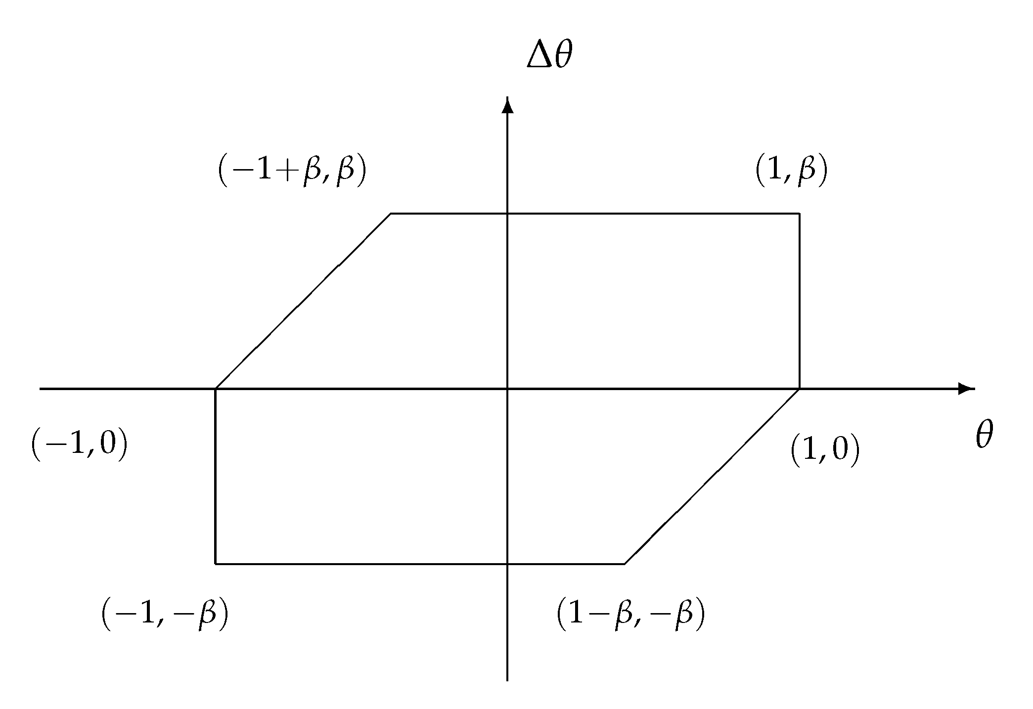
The problem to be addressed is the design of robust ${\mathcal{H}}_{\infty }$ filters with a minimised upper bound γ on $\parallel {\mathcal{G}}_{we}{\parallel }_{\infty }$ for different values of β while considering different values of filter order, $r_f$ and complexity of the Lyapunov matrix $P\left(\theta \right)$. Note that since the one-step-ahead state matrix $E\left(\theta \right)$ is affected by the uncertain parameter θ, to the best of the authors’ knowledge, this problem cannot be solved by existing results in the literature. However, Theorems 1 and 2 can handle this problem. First, Theorems 1 and 2 have been applied to design filters as in (3) and (4) of orders $r_f=i,i=1,2,3,4$. In the case of Theorem 1, either a constant matrix $P\left(\theta \right)=P_0$ or an affine matrix function $P\left(\theta \right)$ was adopted, whereas a $P\left(\theta \right)$ quadratic in θ was used in connection with Theorem 2. Moreover, for both theorems the cases of $\beta =0$ and $\beta =2$ have been considered, which correspond to, respectively, a constant parameter θ and a time-varying $\theta \left(k\right)$ with the maximum allowed variation (i.e, $|\Delta \theta (k\left)\right|\le 2$). Table 1 presents the minimum achieved noise attenuation level γ for the latter cases. Note that the filters have been designed using the consistent polytope $\mathcal{X}$ for $(\theta ,\Delta \theta )$ shown in Figure 1.

Table 1. Minimum achieved upper bound γ on $\parallel {\mathcal{G}}_{we}{\parallel }_{\infty }$ for Example 1.

Filter	Theorem 1	Theorem 1	Theorem 2
Order	$\mathit{P}\left(\mathit{\theta }\right)={\mathit{P}}_0$	$\mathit{P}\left(\mathit{\theta }\right)$ Affine in θ	$\mathit{P}\left(\mathit{\theta }\right)$ Quadratic in θ
$r_f$	$\Delta \theta =0$ $\left|\Delta \theta \right|\le 2$	$\Delta \theta =0$ $\left|\Delta \theta \right|\le 2$	$\Delta \theta =0$ $\left|\Delta \theta \right|\le 2$
4	3.7724   3.9020	3.2770   3.8375	2.9161   3.7988
3	3.7725   3.9020	3.2823   3.8523	2.9975   3.8467
2	3.8338   3.9456	3.5025   3.9164	3.4438   3.8562
1	3.9336   4.0687	3.5066   4.0273	3.4986   3.9096

Figure 1. Consistent polytope $\mathcal{X}$ for $(\theta ,\Delta \theta )$.

From the results in Table 1, it turns out that the filter performance improves as the filter order increases, irrespective of the complexity of the Lyapunov matrix $P\left(\theta \right)$. In addition, for a given β and a given filter order, note that the greater the generalised Lyapunov function’s complexity, the better the filter’s performance. For illustration purposes, for $r_f=4$ and $|\Delta \theta (k\left)\right|\le 2$, the state-space matrices of the filter obtained with Theorem 2 are as follows:

$$\begin{array}{c}{E}_f=I_4,A_f=\left[\begin{array}{cccc}\hfill -0.0560& \hfill 0.4685& \hfill 0.8677& \hfill 0.6506\\ \hfill 0.4691& \hfill -0.3655& \hfill -0.7864& \hfill 0.1219\\ \hfill -0.7155& \hfill 0.3410& \hfill 05649& \hfill 0.8638\\ \hfill -0.0530& \hfill 0.0642& \hfill 0.1225& \hfill 0.0231\end{array}\right],\\ B_f=\left[\begin{array}{ccc}\hfill 0.1175& \hfill -0.3048& \hfill -0.0658\\ \hfill -0.4615& \hfill -1.4818& \hfill -1.3903\\ \hfill 0.8018& \hfill 0.6089& \hfill 0.9435\\ \hfill 0.0455& \hfill 0.2209& \hfill 0.1989\end{array}\right],\\ C_f=\left[\begin{array}{cccc}\hfill 0.3466& \hfill -0.1248& \hfill -0.1685& \hfill -0.3708\\ \hfill -0.0132& \hfill 0.0499& \hfill 0.0699& \hfill 0.0599\\ \hfill 0.1812& \hfill -0.1150& \hfill -0.1633& \hfill -0.5210\end{array}\right],\\ D_f=\left[\begin{array}{ccc}\hfill 0.5981& \hfill -0.5655& \hfill -0.5832\\ \hfill -0.0884& \hfill 0.8135& \hfill -0.1653\\ \hfill 0.0164& \hfill -0.0773& \hfill 0.7886\end{array}\right].\\ \end{array}$$

On the other hand, when Theorem 2 is applied with $r_f=2$ and $|\Delta \theta (k\left)\right|\le 2$, the following state-space filter matrices have been obtained:

$$\begin{array}{c}\\ E_f=\left[\begin{array}{cccc}1& 0& 0& 0\\ 0& 1& 0& 0\\ 0& 0& 0& 0\\ 0& 0& 0& 0\end{array}\right],\\ A_f=\left[\begin{array}{cccc}0.0841& 0.1054& 0& 0\\ 0.0923& 0.0025& 0& 0\\ -0.1545& -0.1037& 0.1& 0\\ -0.0017& -0.0253& 0& 0.1\end{array}\right],\\ B_f=\left[\begin{array}{ccc}-0.0693& -0.4041& -0.3999\\ 0.1762& -0.1126& 0.0137\\ 0.1567& -0.0916& 0.1611\\ -0.0351& 0.0312& 0.0250\end{array}\right],\end{array}$$

$$\begin{array}{c}{C}_f=\left[\begin{array}{cccc}0.2015& 0.0460& 0& 0\\ 0.0484& 0.0604& 0& 0\\ 0.0787& -0.0205& 0& 0\end{array}\right],\\ D_f=\left[\begin{array}{ccc}0.5726& -0.5800& -0.6806\\ -0.1947& 0.7000& -0.3094\\ -0.1051& -0.1298& 0.8022\end{array}\right].\\ \end{array}$$

Note that the latter filter is input-to-output equivalent to a 2nd-order filter with the following state space realisation:

$$\left\{\begin{array}{cc}\hfill {\widehat{x}}_f(k+1)& ={\widehat{A}}_f{\widehat{x}}_f\left(k\right)+{\widehat{B}}_{f}y\left(k\right),\hfill \\ \hfill s_f\left(k\right)& ={\widehat{C}}_f\left(k\right){\widehat{x}}_f\left(k\right)+{\widehat{D}}_{f}y\left(k\right),\hfill \end{array}\right.$$

where

$$\begin{array}{c}{\widehat{A}}_f = \left[\begin{array}{cc}0.0841& 0.1054\\ 0.0923& 0.0025\end{array}\right],{\widehat{B}}_f = \left[\begin{array}{ccc}-0.0693& -0.4041& -0.3999\\ 0.1762& -0.1126& 0.0137\end{array}\right],\\ {\widehat{C}}_f = \left[\begin{array}{cc}0.2015& 0.0460\\ 0.0484& 0.0604\\ 0.0787& -0.0205\end{array}\right],{\widehat{D}}_f = \left[\begin{array}{ccc}0.5726& -0.5800& -0.6806\\ -0.1947& 0.7000& -0.3094\\ -0.1051& -0.1& 0.8022\end{array}\right].\end{array}$$

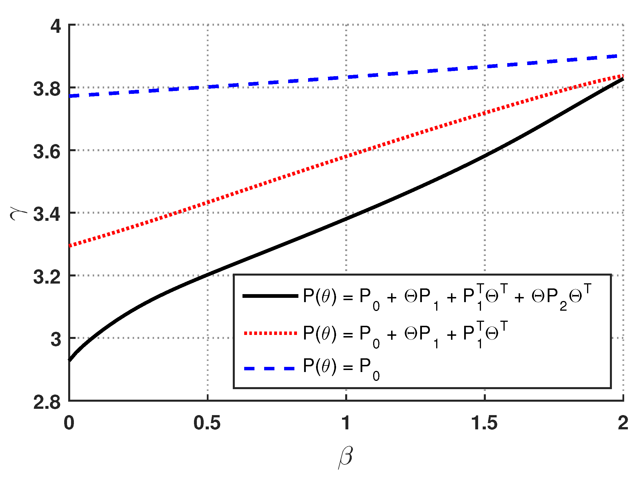
Next, filters with $r_f=4$, i.e., $E_f=I_4$, have been designed with Theorem 2 for different values of β and considering constant, affine and quadratic Lyapunov matrices. Figure 2 displays the minimum achieved upper bound γ on $\parallel {\mathcal{G}}_{we}\parallel$ versus β. Clearly a quadratic Lyapunov matrix function $P\left(\theta \right)$ delivers a better performance, particularly for slow parameter variations.

Figure 2. Minimum achieved upper bound γ on $\parallel {\mathcal{G}}_{we}{\parallel }_{\infty }$ versus β for Example 1 with $r_f=4$, $\left|\theta \right|\le 1$ and $\left|\Delta \theta \right|\le \beta$.

In order to evaluate the computational cost of the proposed filter design methods, Table 2, Table 3 and Table 4 present a relationship between the proposed results and some key variables to evaluate the computational complexity. Precisely, considering different complexity of the Lyapunov function and filter order, Table 2 shows the number of constraints, while Table 3 presents the dimensions of SDP (semidefinite programming) variables (i.e., the number of SDP blocks). The resulting CPU times are given in Table 4. Notice that the use of more complex Lyapunov functions (to derive less conservative results) implies an exponential increase of the computational burden.

Table 2. Numbers of constraints for Example 1.

Filter	Theorem 1	Theorem 1	Theorem 2
Order ${\mathit{r}}_{\mathit{f}}$	$\mathit{P}\left(\mathit{\theta }\right)={\mathit{P}}_0$	$\mathit{P}\left(\mathit{\theta }\right)$ Affine in θ	$\mathit{P}\left(\mathit{\theta }\right)$ Quadratic in θ
4	238	274	2176
3	246	282	2208
2	254	290	2240
1	262	298	2272

Table 3. Numbers and sizes of LMIs (NoL and SoL, respectively) for Example 1.

	Theorem 1	Theorem 1	Theorem 2
	$\mathit{P}\left(\mathit{\theta }\right)={\mathit{P}}_0$	$\mathit{P}\left(\mathit{\theta }\right)$ Affine in θ	$\mathit{P}\left(\mathit{\theta }\right)$ Quadratic in θ
	$\Delta \mathbf{\theta }=\mathbf{0}$   $\left|\Delta \mathbf{\theta }\right|\le \mathbf{2}$	$\Delta \mathbf{\theta }=\mathbf{0}$   $\left|\Delta \mathbf{\theta }\right|\le \mathbf{2}$	$\Delta \mathbf{\theta }=\mathbf{0}$   $\left|\Delta \mathbf{\theta }\right|\le \mathbf{2}$
NoL	2    4	2    4	4    8
SoL	58   116	58   116	142    284

Table 4. Computational time in seconds for Example 1.

Filter	Theorem 1	Theorem 1	Theorem 2
Order	$\mathit{P}\left(\mathit{\theta }\right)={\mathit{P}}_0$	$\mathit{P}\left(\mathit{\theta }\right)$ Affine in θ	$\mathit{P}\left(\mathit{\theta }\right)$ Quadratic in θ
${\mathit{r}}_{\mathit{f}}$	$\Delta \mathbf{\theta }=\mathbf{0}$  $\left|\Delta \mathbf{\theta }\right|\le \mathbf{2}$	$\Delta \mathbf{\theta }=\mathbf{0}$  $\left|\Delta \mathbf{\theta }\right|\le \mathbf{2}$	$\Delta \mathbf{\theta }=\mathbf{0}$  $\left|\Delta \mathbf{\theta }\right|\le \mathbf{2}$
4	1.73  2.56	1.79  2.58	25.88  60.11
3	1.77  2.61	1.81  2.64	35.47  73.01
2	1.80  2.69	1.86  2.81	47.04  80.01
1	1.82  2.72	1.89  2.90	64.61  89.06

Example 2.

Consider the uncertain discrete-time descriptor system as in (1) with the following matrices:

$$\begin{array}{cc}\hfill E\left(\theta \right)& =\left[\begin{array}{ccc}1+0.01\theta & 0& 0\\ 0& 0& 0\\ 0& 1-0.02\theta & 0\end{array}\right],\hfill \end{array}$$

$$\begin{array}{cc}\hfill A\left(\theta \right)& =\left[\begin{array}{ccc}0.51+0.002\theta & 0.32& 0.20-0.004\theta \\ -0.31+0.001\theta & -0.21& 0.15-0.002\theta \\ -0.10& -0.10& -0.40\end{array}\right],\hfill \end{array}$$

(48)

$$\begin{array}{cc}\hfill B\left(\theta \right)& ={\left[\begin{array}{ccc}0.01+0.02\theta & 0.20+0.01\theta & -0.10\end{array}\right]}^T,\hfill \\ \hfill C_y\left(\theta \right)& =\left[\begin{array}{ccc}0.50+0.0002\theta & 0.30& 0.20-0.0004\theta \end{array}\right],\hfill \\ \hfill C_s\left(\theta \right)& =\left[\begin{array}{ccc}0.50+0.004\theta & 0& 0.10-0.008\theta \end{array}\right],\hfill \\ \hfill D_y\left(\theta \right)& =0.1+0.002\theta ,D_s\left(\theta \right)=0.05+0.04\theta ,\hfill \end{array}$$

where $\theta \left(k\right)$ is a scalar time-varying uncertain parameter satisfying $\left|\theta \right(k\left)\right|\le 1$. Note that for all $\theta \ne -100$ and $\theta \ne 50$, $\mathrm{rank}\left\{E\left(\theta \right)\right\}=2$, and the matrix $S\left(\theta \right)$ satisfying Assumption 1 is as follows:

$$S\left(\theta \right)\equiv {\left[\begin{array}{ccc}0& -1& 0\end{array}\right]}^T.$$

(49)

Firstly, robust ${\mathcal{H}}_{\infty }$ filters as in (3) of different orders, $r_f$, have been designed considering that $|\Delta \theta (k\left)\right|\le \beta$ with $\beta =0$ and $\beta =2$. Theorems 1 and 2 have been applied to design augmented-order, full-order and reduced-order filters, i.e. with $r_f=3$, $r_f=2$ and $r_f=1$, respectively. Table 5 displays the achieved results with optimised scalars μ and ϵ and considering different complexities of the Lyapunov matrix function $P\left(\theta \right)$, namely, parameter independent $P\left(\theta \right)\equiv P_0$, affine in θ and quadratic in θ. From these results, similar to Example 1, the use of more complex generalised Lyapunov functions with a larger filter order leads to less conservative results. To the best of the authors’ knowledge, such filter designs cannot be accomplished with ${\mathcal{H}}_{\infty }$ filtering methods that exist in the literature.

Table 5. Minimum achieved upper bound γ on $\parallel {\mathcal{G}}_{we}{\parallel }_{\infty }$ for Example 2 with an uncertain matrix $E\left(\theta \right)$.

Filter	Theorem 1	Theorem 1	Theorem 2
Order	$\mathit{P}={\mathit{P}}_0$	$\mathit{P}\left(\mathit{\theta }\right)$ Affine in θ	$\mathit{P}\left(\mathit{\theta }\right)$ Quadratics in θ
${\mathit{r}}_{\mathit{f}}$	$\Delta \mathbf{\theta }=\mathbf{0}$  $|\Delta \mathbf{\theta }|\le \mathbf{2}$	$\Delta \mathbf{\theta }=\mathbf{0}$  $|\Delta \mathbf{\theta }|\le \mathbf{2}$	$\Delta \mathbf{\theta }=\mathbf{0}$  $|\Delta \mathbf{\theta }|\le \mathbf{2}$
3	0.0666  0.0678	0.0626  0.0670	0.0622  0.0667
2	0.0669  0.0678	0.0644  0.0673	0.0640  0.0670
1	0.0669   0.0678	0.0647   0.0673	0.0642   0.0672

Next, for comparison purposes with the robust ${\mathcal{H}}_{\infty }$ filtering method proposed in [12], which has considered a descriptor system with norm-bounded uncertainty but an uncertainty-free one-step-ahead state matrix E, hereafter it is assumed that

$$E\left(\theta \right)\equiv \left[\begin{array}{ccc}1& 0& 0\\ 0& 0& 0\\ 0& 1& 0\end{array}\right].$$

(50)

To this end, note that the system matrices $A\left(\theta \right)$, $B\left(\theta \right)$, $C_y\left(\theta \right)$, $C_s\left(\theta \right)$, $D_y\left(\theta \right)$ and $D_s\left(\theta \right)$ in (48) can be decomposed as follows:

$$\begin{array}{c}A\left(\theta \right)=A_0+\Delta A\left(\theta \right),B\left(\theta \right)=B_0+\Delta B\left(\theta \right),\\ C_y\left(\theta \right)=C_{y0}+\Delta C_y\left(\theta \right),C_s\left(\theta \right)=C_{s0}+\Delta C_s\left(\theta \right),\\ D_y\left(\theta \right)=D_{y0}+\Delta D_y\left(\theta \right),D_s\left(\theta \right)=D_{s0}+\Delta D_s\left(\theta \right),\end{array}$$

where $\Delta A\left(\theta \right)$, $\Delta B\left(\theta \right)$, $\Delta C_y\left(\theta \right)$, $\Delta C_s\left(\theta \right)$, $\Delta D_y\left(\theta \right)$ and $\Delta D_s\left(\theta \right)$ are norm-bounded uncertainty given by

$$\left[\begin{array}{cc}\Delta A\left(\theta \right)& \Delta B\left(\theta \right)\\ \Delta C_y\left(\theta \right)& \Delta D_y\left(\theta \right)\\ \Delta C_s\left(\theta \right)& \Delta D_s\left(\theta \right)\end{array}\right]=\left[\begin{array}{c}{M}_1\\ M_2\\ M_3\end{array}\right]F\left(\theta \right)\left[\begin{array}{cc}{N}_1& N_2\end{array}\right],$$

with

$$\begin{array}{ccc}& M_1={\left[\begin{array}{ccc}0.2& 0.1& 0\end{array}\right]}^T,N_1=\left[\begin{array}{ccc}0.01& 0& -0.02\end{array}\right],& \\ & M_2=0.02,N_2=0.1,M_3=0.4,& \end{array}$$

and $F\left(\theta \right)=\theta$, which satisfies ${\left|F\left(\theta \right)\right|}^2\le 1$, whereas the matrices $A_0$, $B_0$, $C_{y0}$, $C_{s0}$, $D_{y0}$ and $D_{s0}$ are trivially obtained.

Theorems 1 and 2 have been applied to design robust ${\mathcal{H}}_{\infty }$ filters as in (3) with $E_f=I_3$ and considering (48) and (50), the matrix $S\left(\theta \right)$ in (49) and $|\Delta \theta (k\left)\right|\le \beta$ for β being either 0 or 2. Table 6 shows the minimum upper bound γ on $\parallel {\mathcal{G}}_{we}{\parallel }_{\infty }$ obtained with these theorems and with Theorem 1 of [12], which provides a necessary and sufficient result assuming a generalised parameter-independent Lyapunov function.

Table 6. Optimized γ for Example 2 with E in (50) and 3rd-order filters.

Theorem 1	Theorem 1	Theorem 1	Theorem 2
[12]	$\mathit{P}\left(\mathit{\theta }\right)={\mathit{P}}_0$	$\mathit{P}\left(\mathit{\theta }\right)$ Affine in θ	$\mathit{P}\left(\mathit{\theta }\right)$ Quadratic in θ
$\forall \Delta \mathbf{\theta }$	$\forall \Delta \mathbf{\theta }$	$\Delta \mathbf{\theta }=\mathbf{0}$   $\left|\Delta \mathbf{\theta }\right|\le \mathbf{2}$	$\Delta \mathbf{\theta }=\mathbf{0}$   $\left|\Delta \mathbf{\theta }\right|\le \mathbf{2}$
0.0645	0.0645	0.0613  0.0645	0.0605  0.0645

Notice that the result of [12] was recovered by Theorems 1 and 2 for $\beta =2$ and outperformed in the case of a constant uncertain parameter (i.e., $\beta =0$), demonstrating the potentials of the proposed robust ${\mathcal{H}}_{\infty }$ filtering methods.

Example 3.

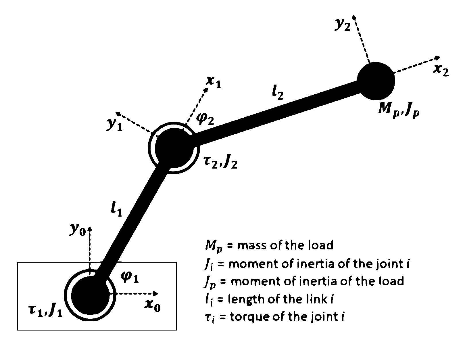
Consider the horizontal 2-DOF robotic manipulator illustrated in Figure 3. According to [17], the system dynamics can be expressed as follows:

$$M\left(\phi \right)\ddot{\phi }+C_c(\phi ,\dot{\phi })\dot{\phi }+D_d\dot{\phi }+K_e\phi =\tau$$

(51)

where $M\left(\phi \right)$, $C_c(\phi ,\dot{\phi })$, $D_d$ and $K_e$ are the inertia, Coriolis (including centripetal effects), damping and stiffness matrices, respectively, whereas φ and τ are the vectors of respectively joint angular positions (${\phi }_1$ and ${\phi }_2$) and torques at the joints (${\tau }_1$ and ${\tau }_2$) in Figure 3 defined by

$$\phi ={\left[\begin{array}{cc}{\phi }_1& {\phi }_2\end{array}\right]}^T,\tau ={\left[\begin{array}{cc}{\tau }_1& {\tau }_2\end{array}\right]}^T.$$

(52)

Figure 3. Horizontal 2-DOF robotic manipulator.

Following the same setup of [17], the matrices $M\left(\phi \right)$, $C_c(\phi ,\dot{\phi })$, $D_d$ and $K_e$ are defined as follows:

$$\begin{array}{ccc}& M\left(\phi \right)=\left[\begin{array}{cc}75.9090+2hcos\left({\phi }_2\right)& 16.5968+hcos\left({\phi }_2\right)\\ 16.5968+hcos\left({\phi }_2\right)& 16.5968\end{array}\right],& \hfill \end{array}$$

(53)

$$\begin{array}{ccc}& C_c(\phi ,\dot{\phi })=\left[\begin{array}{cc}-2hsin\left({\phi }_2\right){\dot{\phi }}_2& -hsin\left({\phi }_2\right){\dot{\phi }}_2\\ hsin\left({\phi }_2\right){\dot{\phi }}_1& 0\end{array}\right],& \hfill \end{array}$$

(54)

$$\begin{array}{ccc}& D_d=\mathrm{diag}\{0.001,0.001\},K_e=0_2,& \hfill \\ & & \hfill \end{array}$$

(55)

where $h=16.0031$. Notice in the above setting that the stiffness matrix $K_e$ is assumed to be zero. Thus, the robotic manipulator model is open-loop unstable. In the sequel, it will be considered that the following stabilising state feedback controller

$$\tau =K_s{\phi }_a,{\phi }_a:=\left[\begin{array}{c}\phi \\ \dot{\phi }\end{array}\right],K_s\in {\mathbb{R}}^{2\times 4},$$

(56)

has been designed to guarantee that the origin of system (51) with (56) is locally asymptotically stable. In particular, $K_s$ was determined such that the spectrum of the linear system obtained from the linear approximation around the origin of (51) with (56) is $\{-1/2,-1/3,-1/4,-1/5\}$, which has led to

$$K_s=\left[\begin{array}{cccc}7.0985& 2.6211& 57.2050& 19.0140\\ 2.0640& 1.6170& 16.9870& 10.7360\end{array}\right].$$

(57)

In this example, we are interested in estimating ${\phi }_1\left(k\right)$ and ${\phi }_2\left(k\right)$ based on noisy measurements of ${\dot{\phi }}_1\left(k\right)$ and ${\dot{\phi }}_2\left(k\right)$, by applying the filtering method of Theorem 1. To this end, the dynamic model given by (51)–(55) is embedded into a continuous-time, linear, parameter-dependent descriptor model and then this latter model is discretised, leading to a descriptor model of the form as in (1). In order to derive a descriptor state-space model, let the following state vector:

$$\begin{array}{cc}\hfill x\left(t\right)=& {\left[\begin{array}{cccccc}{x}_1\left(t\right)& x_2\left(t\right)& x_3\left(t\right)& x_4\left(t\right)& x_5\left(t\right)& x_6\left(t\right)\end{array}\right]}^T\hfill \\ \hfill :=& {\left[\begin{array}{cccccc}{\phi }_1\left(t\right)& {\phi }_2\left(t\right)& {\dot{\phi }}_1\left(t\right)& {\dot{\phi }}_2\left(t\right)& cos\left(x_2\left(t\right)\right)& x_6\left(t\right)\end{array}\right]}^T,\hfill \\ \hfill & \hfill \end{array}$$

where $x_6$ is an algebraic variable to be defined later in the example. In view of the above definition, the dynamics of the robotic manipulator can be cast as follows:

$$\begin{array}{cc}& {\dot{x}}_1=x_3,{\dot{x}}_2=x_4,\hfill \\ & m_{11}\left(x_5\right){\dot{x}}_3+m_{12}\left(x_5\right){\dot{x}}_4-h(2x_3+x_4)x_{4}sin\left(x_2\right)+0.001x_3={\tau }_1\hfill \\ & m_{21}\left(x_5\right){\dot{x}}_3+m_{22}{\dot{x}}_4+h{x}_3^{2}sin\left(x_2\right)+0.001x_4={\tau }_2,\hfill \\ & {\dot{x}}_5=-x_{4}sin\left(x_2\right),\hfill \\ & \hfill \end{array}$$

(58)

where

$$\begin{array}{c}{m}_{11}\left(x_5\right)=75.9090+2h{x}_5,m_{22}=16.5968,\\ m_{12}\left(x_5\right)=m_{21}\left(x_5\right)=16.5968+h{x}_5.\end{array}$$

Now, defining the following parameter vector:

$$\begin{array}{cc}\hfill \theta =& {\left[\begin{array}{ccccc}{\theta }_1& {\theta }_2& {\theta }_3& {\theta }_4& {\theta }_5\end{array}\right]}^T\hfill \\ \hfill :=& {\left[\begin{array}{ccccc}sin\left(x_2\right)& x_3& x_4& x_5& x_6\end{array}\right]}^T,x_6={\theta }_1{x}_3,\hfill \\ & \hfill \end{array}$$

and since $x_{3}sin\left(x_2\right)={\theta }_5$, the following continuous-time, linear, parameter-dependent descriptor model for the 2-DOF robotic manipulator along with noisy measurements of ${\dot{\phi }}_1$ and ${\dot{\phi }}_2$ is readily obtained from (58):

$$\left\{\begin{array}{cc}\hfill E\left(\theta \left(t\right)\right)\dot{x}\left(t\right)& =A_c\left(\theta \left(t\right)\right)x\left(t\right)+B_{c}u\left(t\right),\hfill \\ \hfill y\left(t\right)& =Cx\left(t\right)+Dw\left(t\right),\hfill \end{array}\right.$$

(59)

where $u={\left[{\tau }_1{\tau }_2\right]}^T$ is the control input, $w={\left[w_1{w}_2\right]}^T$ is the measurement noise, $y={\left[y_1{y}_2\right]}^T={\left[{\dot{\phi }}_1{\dot{\phi }}_2\right]}^T$ is the output measurement and

$$\begin{array}{c}E\left(\theta \right)=\left[\begin{array}{ccc}{I}_2& 0_2& 0_2\\ 0_2& {\Pi }_1\left(\theta \right)& {\Pi }_2\left(\theta \right)\\ 0_2& 0_2& {\Pi }_3\end{array}\right],A_c\left(\theta \right)=\left[\begin{array}{ccc}{0}_2& I_2& 0_2\\ 0_2& {\Pi }_4\left(\theta \right)& 0_2\\ 0_2& {\Pi }_5\left(\theta \right)& {\Pi }_6\end{array}\right],\\ B_c={\left[\begin{array}{ccc}{0}_2& I_2& 0_2\end{array}\right]}^T, C = \left[\begin{array}{ccc}{0}_2& I_2& 0_2\end{array}\right], D = 0.1I_2,\end{array}$$

with

$$\begin{array}{c}{\Pi }_1\left(\theta \right)=\left[\begin{array}{cc}{m}_{11}\left({\theta }_4\right)& m_{12}\left({\theta }_4\right)\\ m_{21}\left({\theta }_4\right)& m_{22}\end{array}\right],{\Pi }_2\left(\theta \right)=\left[\begin{array}{cc}2h{\theta }_2+h{\theta }_3& 0\\ 0& 0\end{array}\right],\\ {\Pi }_3=\left[\begin{array}{cc}1& 0\\ 0& 0\end{array}\right],{\Pi }_4\left(\theta \right)=\left[\begin{array}{cc}-0.001& 0\\ -h{\theta }_5& -0.001\end{array}\right],\\ {\Pi }_5\left(\theta \right)=\left[\begin{array}{cc}0& -{\theta }_1\\ -{\theta }_1& 0\end{array}\right],{\Pi }_6=\left[\begin{array}{cc}0& 0\\ 0& 1\end{array}\right].\end{array}$$

Next, system (59) is discretised using a forward finite difference (Euler’s method) with a sampling period $T_s=0.01$ seconds leading to the following discrete-time descriptor model:

$$\left\{\begin{array}{ccc}\hfill E\left(\theta \left(k\right)\right)x(k+1)& =& A\left(\theta \left(k\right)\right)x\left(k\right)+B\left(\theta \left(k\right)\right)w\left(k\right),\hfill \\ \hfill y\left(k\right)& =& C_y\left(\theta \left(k\right)\right)x\left(k\right)+D_y\left(\theta \left(k\right)\right)w\left(k\right),\hfill \end{array}\right.$$

(60)

where $A\left(\theta \right)=E\left(\theta \right)+T_s(A_c\left(\theta \right)+B_{c}K)$, $B\left(\theta \right)=0$, $C_y\left(\theta \right)=C$ and $D_y\left(\theta \right)=D$, with K being a constant stabilising state-feedback gain given by $K=\left[\begin{array}{cc}{K}_s& 0_2\end{array}\right]$. In addition, since in this example we aim at estimating ${\phi }_1\left(k\right)$ and ${\phi }_2\left(k\right)$, we set

$$s\left(k\right)={\left[\begin{array}{cc}{s}_1\left(k\right)& s_2\left(k\right)\end{array}\right]}^T:=C_s\left(\theta \left(k\right)\right)x\left(k\right),$$

(61)

where

$$C_s\left(\theta \left(k\right)\right)=\left[\begin{array}{ccc}{I}_2& 0_2& 0_2\end{array}\right].$$

Moreover, it is considered that ${\theta }_1,\dots ,{\theta }_5$ are time-varying uncertain parameters with admissible values given by:

$$|{\theta }_1|\le 1,|{\theta }_4|\le 1,|{\theta }_2|\le 1.75,|{\theta }_3|\le 1.75,|{\theta }_5|\le 1.75.$$

(62)

In the above, the first two bounds follow from the limits of sine and cosine functions and the remaining ones are obtained from physical limitations of the system states. Additionally, assuming no prior information on the parameters’ variation $\Delta {\theta }_i\left(k\right):={\theta }_i\left(k\right)-{\theta }_i(k-1)$, we consider the maximum admissible parameter variation, i.e, $|\Delta {\theta }_i|\le 2{\theta }_i,i=1,\dots ,5$. It should be noted that the matrix ${\Pi }_1\left(\theta \right)$ is non-singular for all ${\theta }_4\in \mathbb{R}$ which, in light of the structure of the matrix ${\Pi }_3$, implies that $\mathrm{rank}\left\{E\right(\theta \left)\right\}=5$ for all admissible θ. Furthermore, a suitable matrix $S\left(\theta \right)$ of Assumption 1 is as below:

$$S\left(\theta \right)\equiv {\left[\begin{array}{ccccc}0& 0& 0& 0& 1\end{array}\right]}^T.$$

Theorem 1 was applied to design strictly proper filters (i.e., with $D_f=0$) with orders $r_f=6$ (augmented-order), $r_f=5$ (full-order) and $r_f=4$ (reduced-order) for the system in (60)–(62). For the augmented-order filter design, Theorem 1 was applied with the parameters $ϵ=0.3187$ and $\mu =0.6937$ and an upper bound $\gamma =9.1350$ for $\parallel {\mathcal{G}}_{we}{\parallel }_{\infty }$ was obtained. On the other hand, the full-order filter was designed with $ϵ=0.4168$ and $\mu =0.7298$, and led to a value of $\gamma =9.8272$. Finally, $ϵ=0.3787$ and $\mu =0.5937$ were used for designing the reduced-order filter and $\gamma =10.5235$ was achieved. As in the previous two examples, it turns out that filters with larger orders lead to improved ${\mathcal{H}}_{\infty }$ performance. For illustration purpose, in the case of the augmented-order filter the following state-space matrices of the filter have been obtained:

$$\begin{array}{c}{E}_f=I_6,\\ A_f=\left[\begin{array}{cccccc}\hfill 0.9997& \hfill -0.0001& \hfill -0.0018& \hfill 0.0010& \hfill -0.0000& \hfill 0.0002\\ \hfill 0.0000& \hfill 0.9998& \hfill 0.0010& \hfill -0.0020& \hfill 0.0000& \hfill -0.0002\\ \hfill 0.0376& \hfill -0.0093& \hfill -0.4267& \hfill 0.0082& \hfill 0.0006& \hfill 0.0010\\ \hfill 0.0296& \hfill 0.1134& \hfill 0.0078& \hfill -0.4358& \hfill -0.0005& \hfill -0.0028\\ \hfill -0.0001& \hfill 0.0001& \hfill -0.0000& \hfill 0.0000& \hfill 0.9846& \hfill 0.0044\\ \hfill 0.0066& \hfill -0.0016& \hfill 0.0000& \hfill 0.0003& \hfill 0.0276& \hfill -0.4736\end{array}\right],\\ B_f=\left[\begin{array}{cc}\hfill -0.0083& \hfill 0.0002\\ \hfill 0.0002& \hfill -0.0083\\ \hfill -0.2820& \hfill 0.0035\\ \hfill 0.0006& \hfill -0.2778\\ \hfill -0.0001& \hfill 0.0001\\ \hfill 0.0040& \hfill -0.0037\end{array}\right],\\ C_f=\left[\begin{array}{cccccc}\hfill -1.2109& \hfill -0.0025& \hfill 0.0002& \hfill -0.0001& \hfill -0.0001& \hfill -0.0001\\ \hfill -0.0038& \hfill -1.2100& \hfill -0.0001& \hfill 0.0010& \hfill 0.0000& \hfill 0.0002\end{array}\right]\end{array}$$

To illustrate the time-domain performance of the designed filters, we have simulated these filters with $y\left(k\right)$ (and $s\left(k\right)$) being obtained by simulating the continuous-time system (59) with $u\left(t\right)=Kx\left(t\right)$ over the time-interval [0, 40s] considering the consistent initial condition

$$x\left(0\right)={\left[\begin{array}{cccccc}\frac{\pi }{4}& \frac{\pi }{6}& 0.25& 0.5& cos\left(\frac{\pi }{6}\right)& 0\end{array}\right]}^T$$

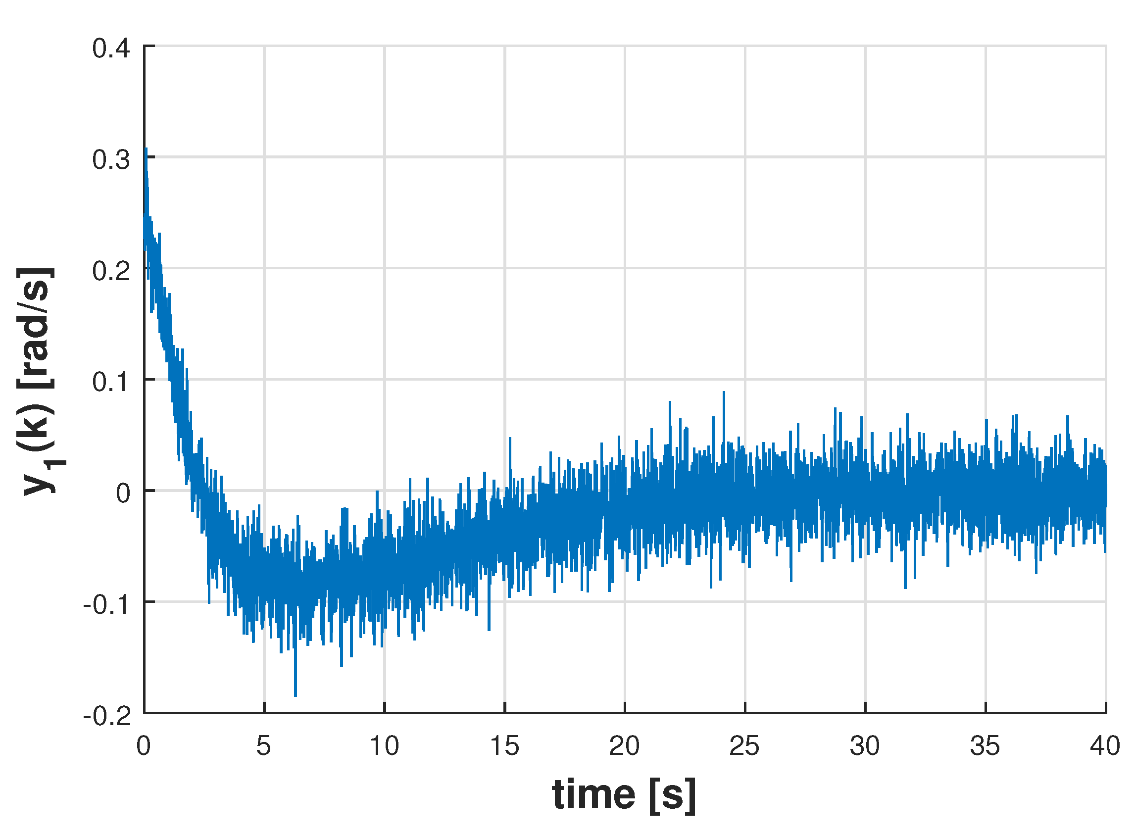
and with $w_1\left(k\right)$ and $w_2\left(k\right)$ being realisations of uncorrelated Gaussian distributed zero-mean white noise sequences with power of $-10$ dB. The resulting measurements $y_1\left(k\right)$ and $y_2\left(k\right)$ are shown in Figure 4 and Figure 5, respectively. Note that the signal-to-noise ratios for $y_1$ and $y_2$ are respectively 1.6589 dB and 5.3977 dB.

Figure 4. Signal $y_1\left(k\right)$.

Figure 5. Signal $y_2\left(k\right)$.

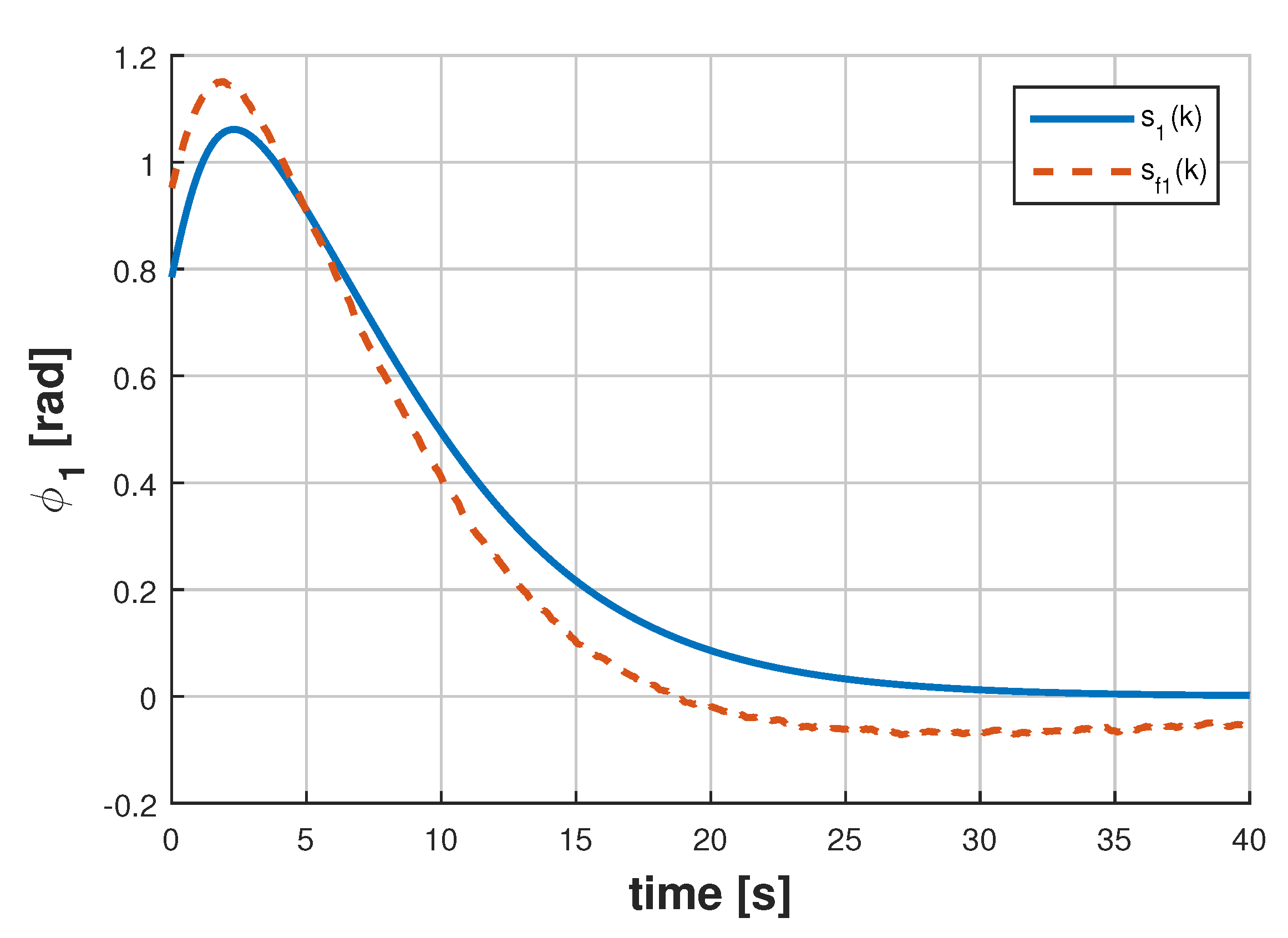
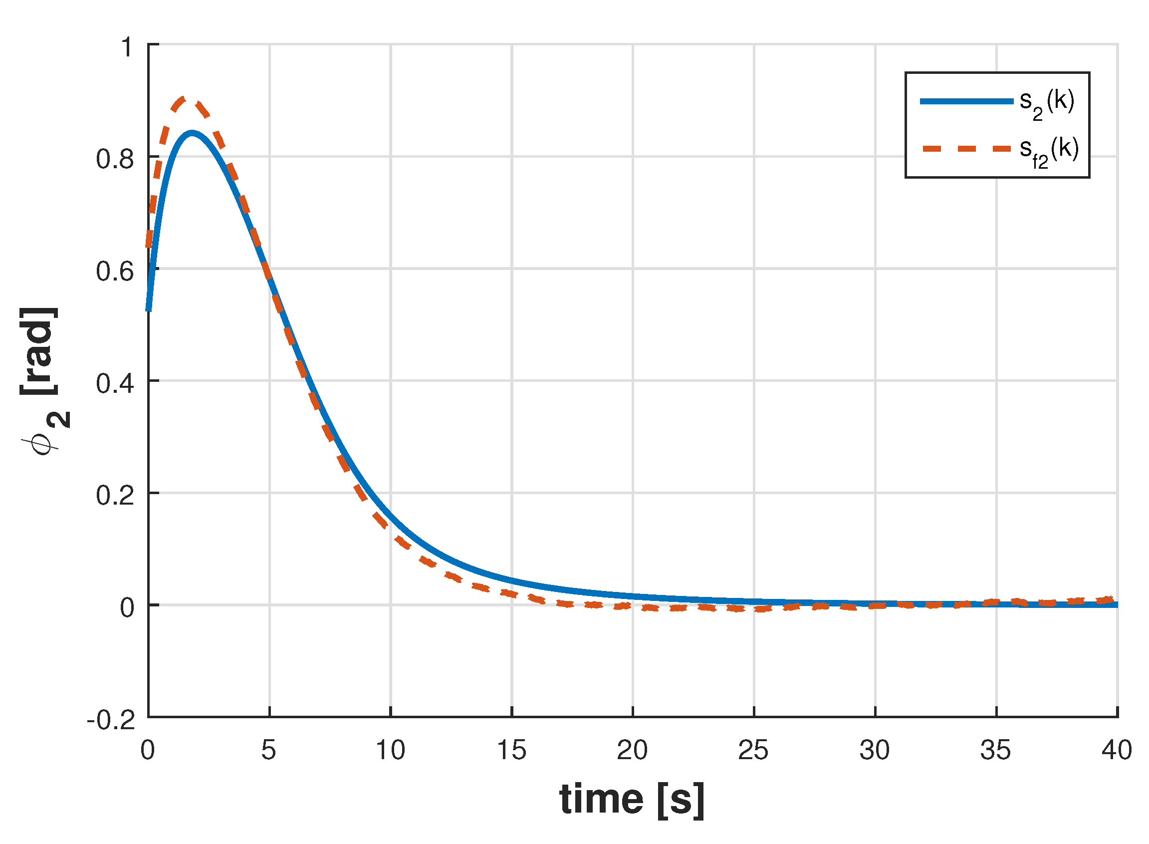
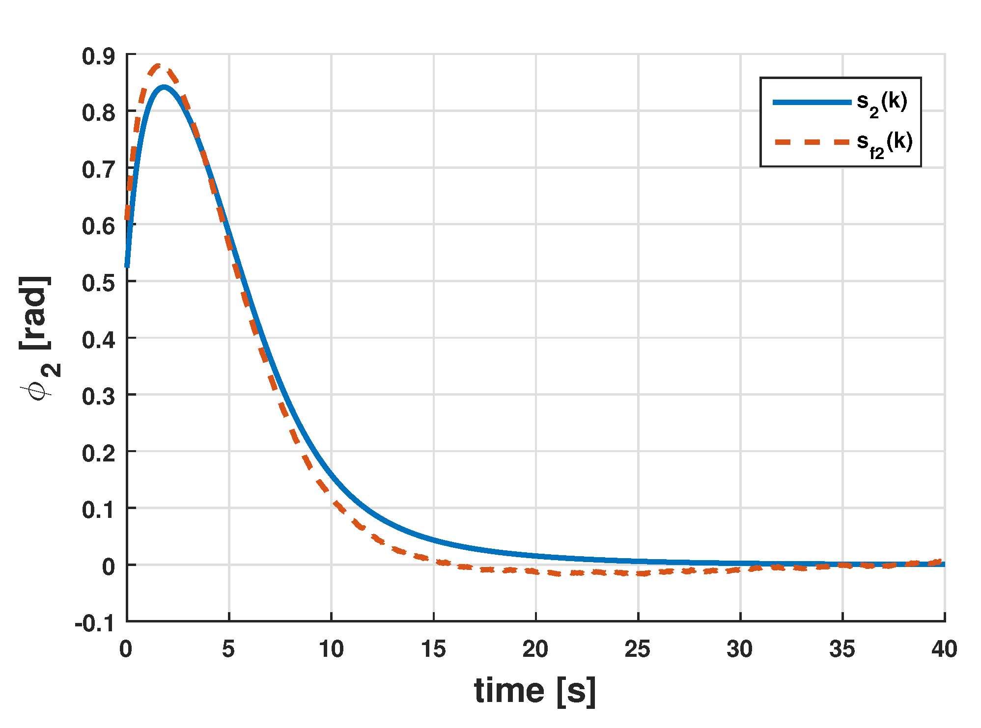
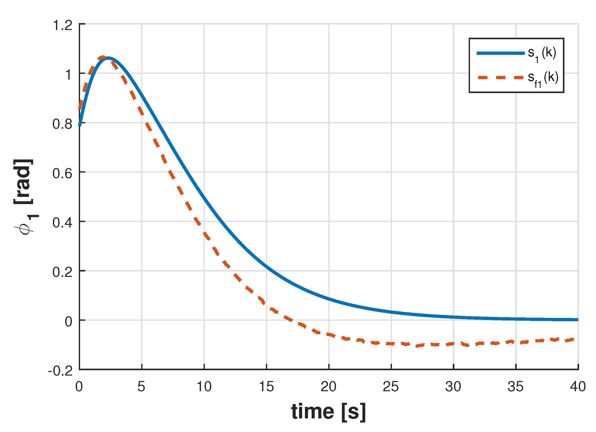
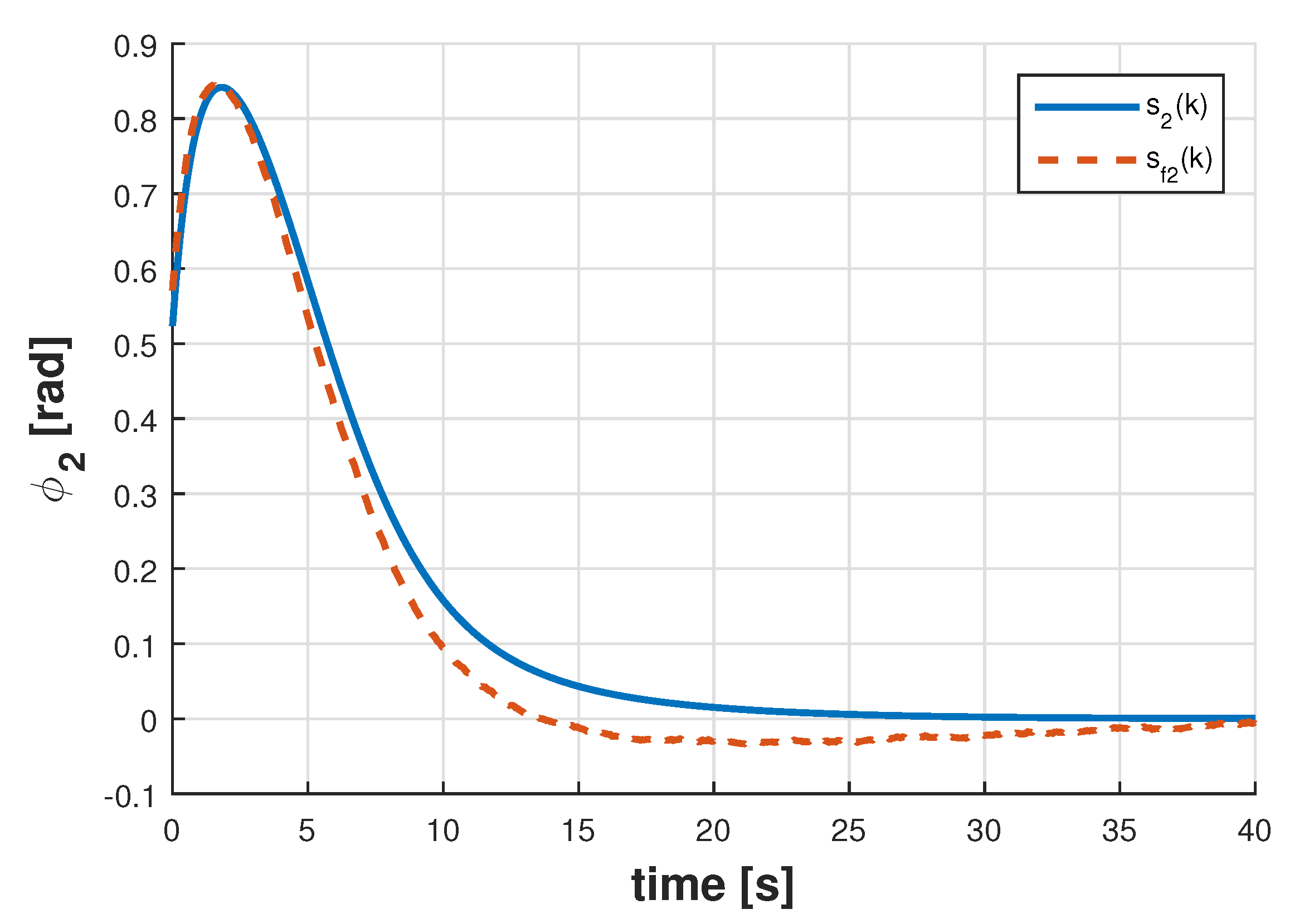
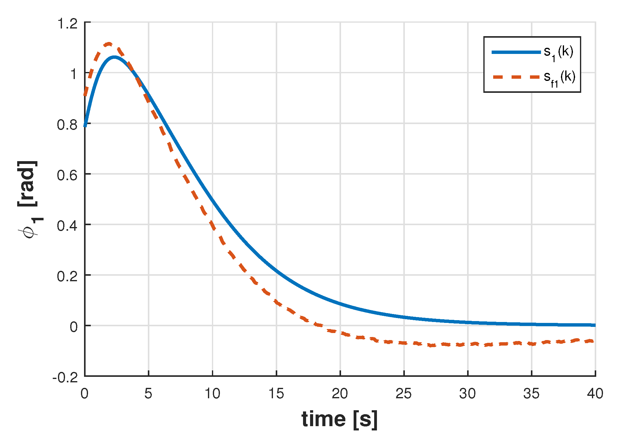
Figure 6 displays the estimate $s_{f1}\left(k\right)$ of the signal $s_1\left(k\right)$ along with $s_1\left(k\right)$, whereas the signals $s_{f2}\left(k\right)$ and $s_2\left(k\right)$ and shown in Figure 7. The results for the full-order filter are displayed in Figure 8 and Figure 9, and in Figure 10 and Figure 11 are depicted the results corresponding to the reduced-order filter. Notice in this particular example that the designed filters have obtained reasonably good estimates of the joint angles despite noisy measurements demonstrating the effectiveness of the proposed approach in a more practical scenario.

Figure 6. Signals $s_1\left(k\right)$ and $s_{f1}\left(k\right)$ for the augmented-order filter.

Figure 7. Signals $s_2\left(k\right)$ and $s_{f2}\left(k\right)$ for the augmented-order filter.

Figure 8. Signals $s_1\left(k\right)$ and $s_{f1}\left(k\right)$ for the full-order filter.

Figure 9. Signals $s_2\left(k\right)$ and $s_{f2}\left(k\right)$ for the full-order filter.

Figure 10. Signals $s_1\left(k\right)$ and $s_{f1}\left(k\right)$ for the reduced-order filter.

Figure 11. Signals $s_2\left(k\right)$ and $s_{f2}\left(k\right)$ for the reduced-order filter.

6. Conclusions

This paper addressed the problem of robust ${\mathcal{H}}_{\infty }$ filtering for discrete linear descriptor systems subject to uncertain parameters which can appear affinely in all the matrices of the system state-space model, including in the one-step-ahead state matrix. It is assumed that the uncertain parameters and their variations have known minimum and maximum values. More specifically, two robust filter design methods were devised in terms of strict LMIs and based on generalised, parameter-dependent Lyapunov functions to ensure a prescribed or optimised upper bound on the ${\ell }_2$-induced gain from the noise signal to the estimation error irrespective of the uncertain parameters. The proposed methodologies allow for designing either standard or descriptor filters having order larger, equal or smaller than the number of dynamic state variables of the system. Three numerical examples have demonstrated the effectiveness of the proposed filter design methods.

Appendix A.1. Proof of Lemma 2

Before presenting the proof of Lemma 2 we recall two canonical state-space representations for discrete-time linear time-varying descriptor systems.

Singular Value Decomposition (SVD) Representation

Given the descriptor system model (7), it is always possible to find $n\times n$ real time-varying matrices $M\left(k\right)$ and $N\left(k\right)$, which are nonsingular for all $k\in {\mathbb{Z}}_0$, such that

$$\overline{E}:=M\left(k\right)E\left(k\right)N\left(k\right)=\left[\begin{array}{cc}{I}_r& 0\\ 0& 0_{n-r}\end{array}\right],\forall k\in {\mathbb{Z}}_0,$$

(A1)

leading to an equivalent representation of system (7) defined as follows and referred to as an SVD representation of (7):

$$\left\{\begin{array}{ccc}\hfill \overline{E}\xi (k+1)& =& \overline{A}\left(k\right)\xi \left(k\right)+\overline{B}\left(k\right)w\left(k\right),\hfill \\ \hfill s\left(k\right)& =& \overline{C}\left(k\right)\xi \left(k\right)+D\left(k\right)w\left(k\right),\hfill \end{array}\right.$$

(A2)

with $\xi \left(k\right)=N^{-1}(k-1)x\left(k\right)$, $N(-1):=N\left(0\right)$, and

$$\overline{A}\left(k\right):=M\left(k\right)A\left(k\right)N(k-1)=\left[\begin{array}{cc}{A}_1\left(k\right)& A_2\left(k\right)\\ A_3\left(k\right)& A_4\left(k\right)\end{array}\right],$$

(A3)

$$\overline{B}\left(k\right):=M\left(k\right)B\left(k\right)=\left[\begin{array}{c}{B}_1\left(k\right)\\ B_2\left(k\right)\end{array}\right],$$

(A4)

$$\overline{C}\left(k\right):=C\left(k\right)N(k-1)=\left[\begin{array}{cc}{C}_1\left(k\right)& C_2\left(k\right)\end{array}\right],$$

(A5)

where the matrices $\overline{A}\left(k\right),\overline{B}\left(k\right)$ and $\overline{C}\left(k\right)$ are partitioned accordingly to $\overline{E}$. The SVD representation in (A2) allows us to state the following causality result for system (7).

Corollary A1.

[24] Consider the system (7) with an SVD representation as in (A2) with matrices given in (A1) and (A3)–(A5). Then, system (7) is causal if and only if the matrix $A_4\left(k\right)$ is nonsingular for all $k\in {\mathbb{Z}}_0$.

Weierstrass Representation

If system (7) is causal, there exists an equivalent state-space representation, denoted as the Weierstrass form [24], given by:

$$\left\{\begin{array}{ccc}\hfill \tilde{E}\zeta (k+1)& =& \tilde{A}\left(k\right)\zeta \left(k\right)+\tilde{B}\left(k\right)w\left(k\right),\hfill \\ \hfill z\left(k\right)& =& \tilde{C}\left(k\right)\zeta \left(k\right)+D\left(k\right)w\left(k\right),\hfill \end{array}\right.$$

(A6)

where $\zeta \left(k\right)={\tilde{N}}^{-1}(k-1)x\left(k\right)$ is the system state, with $\tilde{N}(-1):=\tilde{N}\left(0\right)$, and the matrices in (A6) are as below:

$$\begin{array}{ccc}\hfill \tilde{E}& =& \tilde{M}\left(k\right)E\left(k\right)\tilde{N}\left(k\right)=\left[\begin{array}{cc}{I}_r& 0\\ 0& 0_{n-r}\end{array}\right],\hfill \end{array}$$

(A7)

$$\begin{array}{ccc}\hfill \tilde{A}\left(k\right)& =& \tilde{M}\left(k\right)A\left(k\right)\tilde{N}(k-1)=\left[\begin{array}{cc}{A}_W\left(k\right)& 0\\ 0& I_{n-r}\end{array}\right],\hfill \end{array}$$

(A8)

$$\begin{array}{ccc}\hfill \tilde{B}\left(k\right)& =& \tilde{M}\left(k\right)B\left(k\right)=\left[\begin{array}{c}{B}_W\left(k\right)\\ A_4^{-1}\left(k\right)B_2\left(k\right)\end{array}\right],\hfill \end{array}$$

(A9)

$$\begin{array}{ccc}\hfill \tilde{C}\left(k\right)& =& C\left(k\right)\tilde{N}(k-1)=\left[\begin{array}{cc}{C}_W\left(k\right)& C_2\left(k\right)\end{array}\right],\hfill \\ & & \hfill \end{array}$$

(A10)

with

$$\left\{\begin{array}{ccc}\hfill A_W\left(k\right)& =& A_1\left(k\right)-A_2\left(k\right)A_4^{-1}\left(k\right)A_3\left(k\right),\hfill \\ \hfill B_W\left(k\right)& =& B_1\left(k\right)-A_2\left(k\right)A_4^{-1}\left(k\right)B_2\left(k\right),\hfill \\ \hfill C_W\left(k\right)& =& C_1\left(k\right)-C_2\left(k\right)A_4^{-1}\left(k\right)A_3\left(k\right),\hfill \end{array}\right.$$

(A11)

and $\tilde{M}\left(k\right)$ and $\tilde{N}\left(k\right)$ are nonsingular $n\times n$ real matrices for all $k\in {\mathbb{Z}}_0$, $A_i\left(k\right),i=1,\dots ,4,B_i\left(k\right)$ and $C_i\left(k\right),i=1,2,$ are the matrices of the SVD representation as given in (A3)–(A5), and where $\tilde{A}\left(k\right),\tilde{B}\left(k\right)$ and $\tilde{C}\left(k\right)$ are partitioned accordingly to $\tilde{E}$. Note that, in light of Corollary A1, the non-singularity of $A_4\left(k\right),\forall k\in {\mathbb{Z}}_0$, is ensured by the causality of system (7).

Proof of Lemma 2. 

$\left(\mathit{i}\right)$ Assume that the conditions of Lemma 2 $\left(i\right)$ hold. Then, it follows from (10) that ${\mathrm{Y}}_1\left(k\right)<0,\forall k\in {\mathbb{Z}}_0$, with $X(k-1)>0$, $\forall k\in {\mathbb{Z}}_0$, which by Lemma 1 implies that the unforced system of (7) is admissible. Now, it will be shown that $\parallel {\mathcal{G}}_{ws}{\parallel }_{\infty }<\gamma$. To this end, consider the following generalised Lyapunov function candidate:

$$V(x,k)=x^T{E}^T(k-1)X(k-1)E(k-1)x$$

and its variation $\Delta V(x,k):=V\left(x\right(k+1),k+1)-V\left(x\right(k),k)$ along the trajectories of system (7). Due to the fact that $E^T\left(k\right)S\left(k\right)=0,\forall k\in {\mathbb{Z}}_0$, then for any bounded matrix $Q\left(k\right)$ of appropriate dimensions it holds that

$$\begin{array}{c}\Delta V(x,k)=x^T(k+1)E^T\left(k\right)X\left(k\right)E\left(k\right)x(k+1)-x^T\left(k\right)E^T(k-1)X(k-1)E(k-1)x\left(k\right)+\hfill \\ \hfill 2x^T(k+1)E^T\left(k\right)S\left(k\right)Q\left(k\right)x\left(k\right).\end{array}$$

(A12)

Considering (7), it can be verified that (A12) can be written as

$$\Delta V(x,k)={\eta }^T\left(k\right)\left[\begin{array}{cc}{\mathrm{Y}}_1\left(k\right)& {\mathrm{Y}}_2^T\left(k\right)\\ {\mathrm{Y}}_2\left(k\right)& {\mathrm{Y}}_3\left(k\right)\end{array}\right]\eta \left(k\right),$$

(A13)

where $\eta \left(k\right)={\left[x^T\left(k\right)w^T\left(k\right)\right]}^T$, ${\mathrm{Y}}_1\left(k\right)$ and ${\mathrm{Y}}_2\left(k\right)$ are as in (11) and (12), respectively, and ${\mathrm{Y}}_3\left(k\right)=B^T\left(k\right)X\left(k\right)B\left(k\right)$. On the other hand, note that applying Schur complements to (10) leads to:

$$\left[\begin{array}{cc}{\mathrm{Y}}_1\left(k\right)& {\mathrm{Y}}_2^T\left(k\right)\\ {\mathrm{Y}}_2\left(k\right)& {\mathrm{Y}}_3\left(k\right)-\gamma I\end{array}\right]+{\gamma }^{-1}\left[\begin{array}{c}{C}^T\left(k\right)\\ D^T\left(k\right)\end{array}\right]\left[\begin{array}{cc}C\left(k\right)& D\left(k\right)\end{array}\right]<0.$$

(A14)

Then, pre- and post-multiplying (A14) by ${\eta }^T\left(k\right)$ and $\eta \left(k\right)$, respectively, and taking (7) and (A13) into account, it follows that

$$\Delta V(x,k)+{\gamma }^{-1}{s}^T\left(k\right)s\left(k\right)-\gamma w^T\left(k\right)w\left(k\right)<0.$$

(A15)

Summing up (A15) from zero to infinity and considering that system (7) is exponentially stable and $E(-1):=E\left(0\right)$, leads to

$${\parallel s\parallel }_2^2-{\gamma }^2{\parallel w\parallel }_2^2<0,\forall w\in {\ell }_2:w\left(k\right)\not\equiv 0,E\left(0\right)x\left(0\right)=0,$$

which implies that $\parallel {\mathcal{G}}_{ws}{\parallel }_{\infty }<\gamma$. $\left(\mathit{ii}\right)$ Firstly, consider an SVD form as in (A2) for system (7) and let the state vector in (A2) be partitioned as follows:

$$\xi \left(k\right)={\left[\begin{array}{cc}{\xi }_1^T\left(k\right)& {\xi }_2^T\left(k\right)\end{array}\right]}^T,{\xi }_1\left(k\right)\in {\mathbb{R}}^r,{\xi }_2\left(k\right)\in {\mathbb{R}}^{n-r}.$$

(A16)

As system (7) is admissible, by Corollary A1 the matrix $A_4\left(k\right)$ in (A3) is nonsingular for all $k\in {\mathbb{Z}}_0$. Due to this fact, the static state variable ${\xi }_2\left(k\right)$ can be eliminated from system (A2) leading to the following equivalent state-space representation for the mapping from w to s of system (7):

$$\begin{array}{cc}\hfill {\xi }_1(k+1)& =A_W\left(k\right){\xi }_1\left(k\right)+B_W\left(k\right)w\left(k\right),\hfill \\ \hfill s\left(k\right)& =C_W\left(k\right){\xi }_1\left(k\right)+D_W\left(k\right)w\left(k\right),\hfill \end{array}$$

(A17)

where $A_W\left(k\right)$, $B_W\left(k\right)$ and $C_W\left(k\right)$ are as in (A11) and

$$D_W\left(k\right)=D\left(k\right)-C_2\left(k\right)A_4^{-1}\left(k\right)B_2\left(k\right).$$

Since system (A17) is exponentially stable and its ${\mathcal{H}}_{\infty }$ norm is smaller than $\gamma$, it follows from the well known bounded real lemma [31] that there exists a matrix $Z\left(k\right)>0,\forall k\in {\mathbb{Z}}_0$, such that:

$$\left[\begin{array}{ccc}{\mathsf{\Psi }}_1\left(k\right)& {\mathsf{\Psi }}_2^T\left(k\right)& C_W^T\left(k\right)\\ {\mathsf{\Psi }}_2\left(k\right)& {\mathsf{\Psi }}_3\left(k\right)& D_W^T\left(k\right)\\ C_W\left(k\right)& D_W\left(k\right)& -\gamma I\end{array}\right]<0,\forall k\in {\mathbb{Z}}_0,$$

(A18)

where

$$\begin{array}{cc}\hfill & \\ \hfill {\mathsf{\Psi }}_1\left(k\right)& =A_W^T\left(k\right)Z(k+1)A_W\left(k\right)-Z\left(k\right),\hfill \\ \hfill {\mathsf{\Psi }}_2\left(k\right)& =B_W^T\left(k\right)Z(k+1)A_W\left(k\right),\hfill \\ \hfill {\mathsf{\Psi }}_3\left(k\right)& =B_W^T\left(k\right)Z(k+1)B_W\left(k\right)-\gamma I.\hfill \\ \hfill \end{array}$$

On the other hand, since system (7) is admissible, it can be represented via a Weierstrass representation as given in (A6)–(A11). To show that there exist matrices $Q\left(k\right)$ and $X(k-1)>0$, $\forall k\in {\mathbb{Z}}_0$, satisfying (10), we will represent the matrices of system (7) in terms of the matrices $\tilde{E}\left(k\right)$, $\tilde{A}\left(k\right)$, $\tilde{B}\left(k\right)$, and $\tilde{C}\left(k\right)$ of the Weierstrass representation as in (A6)–(A10), namely:

$$\left\{\begin{array}{c}E\left(k\right)={\tilde{M}}^{-1}\left(k\right)\tilde{E}{\tilde{N}}^{-1}\left(k\right),\hfill \\ A\left(k\right)={\tilde{M}}^{-1}\left(k\right)\tilde{A}\left(k\right){\tilde{N}}^{-1}(k-1),\hfill \\ B\left(k\right)={\tilde{M}}^{-1}\left(k\right)\tilde{B}\left(k\right),C\left(k\right)=\tilde{C}\left(k\right){\tilde{N}}^{-1}(k-1),\hfill \end{array}\right.$$

(A19)

and apply appropriate congruence transformations to (10), as will be shown in the following. Since from (A19), $E\left(k\right)={\tilde{M}}^{-1}\left(k\right)\mathrm{diag}\{I_r,0_{n-r}\}{\tilde{N}}^{-1}\left(k\right)$, a suitable matrix $S\left(k\right)\in {\mathbb{R}}^{n\times (n-r)}$ such that $\mathrm{rank}\left\{S\right(k\left)\right\}=n-r$ and $E^T\left(k\right)S\left(k\right)=0$, for all $k\in {\mathbb{Z}}_0$, is as follows:

$$S\left(k\right)={\tilde{M}}^T\left(k\right)\left[\begin{array}{c}{0}_{r\times (n-r)}\\ I_{n-r}\end{array}\right]\tilde{W}\left(k\right),$$

(A20)

where $\tilde{W}\left(k\right)$ is any $(n-r)\times (n-r)$ nonsingular matrix for all $k\in {\mathbb{Z}}_0$. In addition, let $\tilde{W}\left(k\right)Q\left(k\right)\tilde{N}(k-1)$ be partitioned as below:

$$\tilde{W}\left(k\right)Q\left(k\right)\tilde{N}(k-1)=\left[\begin{array}{cc}{\tilde{Q}}_1\left(k\right)& {\tilde{Q}}_2\left(k\right)\end{array}\right],$$

(A21)

where ${\tilde{Q}}_1\left(k\right)\in {\mathbb{R}}^{(n-r)\times r}$ and ${\tilde{Q}}_2\left(k\right)\in {\mathbb{R}}^{(n-r)\times (n-r)}$. Moreover, let the following matrix:

$$\tilde{X}\left(k\right):={\tilde{M}}^{-T}\left(k\right)X\left(k\right){\tilde{M}}^{-1}\left(k\right)=\left[\begin{array}{cc}{\tilde{X}}_1\left(k\right)& {\tilde{X}}_2\left(k\right)\\ {\tilde{X}}_2^T\left(k\right)& {\tilde{X}}_4\left(k\right)\end{array}\right],$$

(A22)

where ${\tilde{X}}_1\left(k\right)\in {\mathbb{R}}^{r\times r}$ and ${\tilde{X}}_4\left(k\right)\in {\mathbb{R}}^{(n-r)\times (n-r)}$. Denoting the left-hand side of (10) by $\widehat{\mathsf{\Gamma }}\left(k\right)$, considering (A19)–(A22) and carrying out lengthy matrix manipulations, it can be shown that:

$${\mathbb{G}}^T\left(k\right)\widehat{\mathsf{\Gamma }}\left(k\right)\mathbb{G}\left(k\right)=\mathsf{\Gamma }\left(k\right),$$

(A23)

with $\mathbb{G}\left(k\right)=\mathrm{diag}\{\tilde{N}(k-1),I_{n_w},I_{n_s}\}$,

$$\mathsf{\Gamma }\left(k\right)=\left[\begin{array}{cccc}{\mathsf{\Gamma }}_{11}\left(k\right)& \star & \star & \star \\ {\mathsf{\Gamma }}_{21}\left(k\right)& {\mathsf{\Gamma }}_{22}\left(k\right)& \star & \star \\ {\mathsf{\Gamma }}_{31}\left(k\right)& {\mathsf{\Gamma }}_{32}\left(k\right)& {\mathsf{\Gamma }}_{33}\left(k\right)& \star \\ C_W& C_2& D& -\gamma I\end{array}\right],$$

$$\begin{array}{cc}\hfill & \\ \hfill {\mathsf{\Gamma }}_{11}\left(k\right)& =A_W^T{\tilde{X}}_1\left(k\right)A_W-{\tilde{X}}_1(k-1),\hfill \\ \hfill {\mathsf{\Gamma }}_{21}\left(k\right)& ={\tilde{X}}_2^T\left(k\right)A_W+{\tilde{Q}}_1\left(k\right),\hfill \\ \hfill {\mathsf{\Gamma }}_{22}\left(k\right)& ={\tilde{X}}_4\left(k\right)+\mathrm{He}\left\{{\tilde{Q}}_2\left(k\right)\right\},\hfill \\ \hfill {\mathsf{\Gamma }}_{31}\left(k\right)& =B_W^T{\tilde{X}}_1\left(k\right)A_W+B_2^T{A}_4^{-T}\left({\tilde{X}}_2^T\left(k\right)A_W+{\tilde{Q}}_1\left(k\right)\right),\hfill \\ \hfill {\mathsf{\Gamma }}_{32}\left(k\right)& =B_W^T{\tilde{X}}_2\left(k\right)+B_2^T{A}_4^{-T}\left({\tilde{X}}_4\left(k\right)+{\tilde{Q}}_2\left(k\right)\right),\hfill \\ \hfill {\mathsf{\Gamma }}_{33}\left(k\right)& =B_W^T{\tilde{X}}_1\left(k\right)B_W+\mathrm{He}\left\{B_2^T{A}_4^{-T}{\tilde{X}}_2^T\left(k\right)B_W\right\}+B_2^T{A}_4^{-T}{\tilde{X}}_4\left(k\right)A_4^{-1}{B}_2-\gamma I,\hfill \end{array}$$

where the argument k of $A_4\left(k\right)$, $A_W\left(k\right)$, $B_2\left(k\right)$, $B_W\left(k\right)$, $C_2\left(k\right)$, $C_W\left(k\right)$ and $D\left(k\right)$ has been omitted.

Post- and pre-multiplying $\mathsf{\Gamma }\left(k\right)$ by

$$\mathbb{H}\left(k\right)=\left[\begin{array}{cccc}{I}_r& 0& 0& 0\\ 0& -A_4^{-1}\left(k\right)B_2\left(k\right)& 0& I_{n-r}\\ 0& I_{n_w}& 0& 0\\ 0& 0& I_{n_s}& 0\end{array}\right]$$

and its transpose, respectively, and setting ${\tilde{X}}_1\left(k\right)=Z(k+1)$, ${\tilde{X}}_2\left(k\right)=0$ and ${\tilde{Q}}_1\left(k\right)=0$, $\forall k\in {\mathbb{Z}}_0$, leads to:

$${\mathbb{H}}^T\left(k\right)\mathsf{\Gamma }\left(k\right)\mathbb{H}\left(k\right)=\left[\begin{array}{cc}\Lambda \left(k\right)& {\tilde{\Lambda }}^T\left(k\right)\\ \tilde{\Lambda }\left(k\right)& {\tilde{X}}_4\left(k\right)+\mathrm{He}\left\{{\tilde{Q}}_2\left(k\right)\right\}\end{array}\right],$$

where $\Lambda \left(k\right)$ denotes the left-hand side of (A18) and

$$\tilde{\Lambda }\left(k\right)=\left[\begin{array}{ccc}0& -{\tilde{Q}}_2^T\left(k\right)A_4\left(k\right)B_2\left(k\right)& C_2^T\left(k\right)\end{array}\right].$$

Next, since the assumption $\mathrm{Ker}\left\{E^T\left(k\right)\right\}\subseteq \mathrm{Ker}\left\{B^T\left(k\right)\right\}$ is equivalent to $B_2\left(k\right)\equiv 0$, whereas $\mathrm{Ker}\left\{E\right(k\left)\right\}\subseteq \mathrm{Ker}\left\{C\right(k+1\left)\right\}$ is equivalent to $C_2\left(k\right)\equiv 0$, and considering that $\Lambda \left(k\right)<0$, $\forall k\in {\mathbb{Z}}_0$, it follows from Schur complements that under either the assumption $\mathrm{Ker}\left\{E^T\left(k\right)\right\}\subseteq \mathrm{Ker}\left\{B^T\left(k\right)\right\},\forall k\in {\mathbb{Z}}_0$, or $\mathrm{Ker}\left\{E\left(k\right)\right\}\subseteq \mathrm{Ker}\left\{C(k+1)\right\},\forall {\mathbb{Z}}_{-1}$, we can choose ${\tilde{Q}}_2\left(k\right)$ and ${\tilde{X}}_4\left(k\right)>0$, with ${\tilde{X}}_4\left(k\right)+\mathrm{He}\left\{{\tilde{Q}}_2\left(k\right)\right\}<0$, $\forall k\in {\mathbb{Z}}_0$, such that ${\mathbb{H}}^T\left(k\right)\mathsf{\Gamma }\left(k\right)\mathbb{H}\left(k\right)<0$, $\forall k\in {\mathbb{Z}}_0$, or equivalently $\widehat{\mathsf{\Gamma }}\left(k\right)<0,\forall k\in {\mathbb{Z}}_0$. Therefore, in light of (A21) and (A22), it follows that (10) is satisfied with the following matrices:

$$Q\left(k\right)={\tilde{W}}^{-1}\left(k\right)\left[\begin{array}{cc}0& {\tilde{Q}}_2\left(k\right)\end{array}\right]{\tilde{N}}^{-1}(k-1),$$

$$X\left(k\right)={\tilde{M}}^T\left(k\right)\mathrm{diag}\left\{{\tilde{X}}_1\left(k\right),{\tilde{X}}_4\left(k\right)\right\}\tilde{M}\left(k\right).$$

□

Appendix A.2. Proof of Lemma 4

Proof of Lemma 4. 

Assume there exist constant matrices $A_f$, $B_f$, $C_f$ and $D_f$, bounded matrix functions $P\left(\theta \right)>0,\forall \theta \in {\mathbb{Z}}_0$, $F\left(\theta \right)$, $G\left(\theta \right)$, $H\left(\theta \right)$ and $R\left(\theta \right)$ satisfying (22) for $E_f=I_n$, and with $G\left(\theta \right)$ being partitioned as follows:

$$G\left(\theta \right)=\left[\begin{array}{cc}{G}_1\left(\theta \right)& G_3\\ G_2\left(\theta \right)& G_4\end{array}\right],$$

(A24)

where $G_1\left(\theta \right),G_2\left(\theta \right)\in {\mathbb{R}}^{n\times n}$ are bounded matrix functions and $G_3,G_4\in {\mathbb{R}}^{n\times n}$ are constant matrices. Notice from (22) that ${\mathsf{\Omega }}_3\left(\theta \right)<0,\forall \theta \in {\mathcal{X}}_0$, and since $P\left(\theta \right)>0,\forall \theta \in {\mathcal{X}}_0$, it follows that $G\left(\theta \right)+G^T\left(\theta \right)>0,\forall \theta \in {\mathcal{X}}_0$, which implies that $G_4$ is nonsingular. Moreover, as (22) is a strict inequality, without loss of generality, the matrix $G_3$ can be assumed to be nonsingular. Next, take the nonsingular matrix U as below:

$$U=\left[\begin{array}{cc}{I}_n& 0_n\\ 0_n& W\end{array}\right],W=G_3{G}_4^{-1},$$

(A25)

and recall that $S_a\left(\theta \right)={\left[\begin{array}{cc}{S}^T\left(\theta \right)& 0_{n\times (n-r)}^T\end{array}\right]}^T$. Hence, by pre- and post-multiplying (22) by $\mathbb{T}=\mathrm{diag}\{U,I,U,U,I\}$ and ${\mathbb{T}}^T$, respectively, and performing straightforward matrix manipulations, it can be shown that (22) is also satisfied with the matrices $A_f$, $B_f$, $C_f$, $D_f$, $F\left(\theta \right)$, $G\left(\theta \right)$, $H\left(\theta \right)$, $P\left(\theta \right)$ and $R\left(\theta \right)$ replaced by respectively ${\breve{A}}_f$, ${\breve{B}}_f$, ${\breve{C}}_f$, ${\breve{D}}_f$, $\breve{F}\left(\theta \right)$, $\breve{G}\left(\theta \right)$, $\breve{H}\left(\theta \right)$, $\breve{P}\left(\theta \right)$ and $\breve{R}\left(\theta \right)$ as below:

$$\begin{array}{c}{\breve{A}}_f=W^{-T}{A}_f{W}^T,{\breve{B}}_f=W^{-T}{B}_f,{\breve{C}}_f=C_f{W}^T,\\ {\breve{D}}_f=D_f,\breve{F}\left(\theta \right)=UF\left(\theta \right)U^T,\breve{G}\left(\theta \right)=UG\left(\theta \right)U^T,\\ \breve{H}\left(\theta \right)=UH\left(\theta \right)U^T,\breve{P}\left(\theta \right)=UP\left(\theta \right)U^T,\breve{R}\left(\theta \right)=R\left(\theta \right)U^T.\end{array}$$

Observe that the filter with state-space realisation $({\breve{A}}_f,{\breve{B}}_f,{\breve{C}}_f,{\breve{D}}_f)$ is similar to the one with realisation $(A_f,B_f,C_f,D)$, and thus both filters are input-to-output equivalent. Note that in view of (A24) and (A25), it turns out that $\breve{G}\left(\theta \right)$ is as follows:

$$\breve{G}\left(\theta \right)=\left[\begin{array}{cc}{G}_1\left(\theta \right)& G_3{G}_4^{-T}{G}_3^T\\ W{G}_2\left(\theta \right)& G_3{G}_4^{-T}{G}_3^T\end{array}\right].$$

Therefore, the proof follows by setting ${\breve{G}}_1\left(\theta \right)=G_1\left(\theta \right)$, ${\breve{G}}_2\left(\theta \right)=W{G}_2\left(\theta \right)$ and ${\breve{G}}_3=G_3{G}_4^{-T}{G}_3^T$. □

References

1. Duan, G.R. Analysis and Design of Descriptor Linear Systems; Springer: New York, NY, USA, 2010. [Google Scholar]
2. Belov, A.A.; Andrianova, O.G.; Kurdyukov, A.P. Control of Discrete-Time Descriptor Systems; Springer: Berlin/Heidelberg, Germany, 2018. [Google Scholar]
3. Xu, S.; Lam, J.; Zou, Y. H filtering for singular systems. IEEE Trans. Autom. Control. 2003, 48, 2217–2222. [Google Scholar]
4. Xu, S.; Lam, J. Robust Control and Filtering of Singular Systems; Springer: Berlin, Germany, 2006. [Google Scholar]
5. Beidaghi, S.; Jalalim, A.; Khaki, A. H filtering for descriptor systems with strict LMI conditions. Automatica 2017, 80, 88–94. [Google Scholar]
6. Yue, D.; Han, Q.L. Robust H filter design of uncertain descriptor systems with discrete and distributed delays. IEEE Trans. Signal Process. 2004, 52, 3200–3212. [Google Scholar] [CrossRef]
7. De Souza, C.E.; Barbosa, K.A.; Xie, L. Robust H filtering for linear descriptor systems with convex bounded uncertainty. In Proceedings of the IEEE International Conference Control and Automation (ICCA), Guangzhou, China, 17–20 October 2007; pp. 47–52. [Google Scholar]
8. Barbosa, K.; Cipriano, A. Robust H filter design for singular systems with time-varying uncertainties. IET Control Theory Appl. 2011, 5, 1085–1091. [Google Scholar] [CrossRef]
9. Lee, C.M.; Fong, I. H filter design for uncertain discrete-time singular systems via normal transformation. Circuits Syst. Signal Process. 2006, 25, 525–538. [Google Scholar] [CrossRef]
10. De Souza, C.E.; Barbosa, K.A.; Fu, M. Robust filtering for uncertain linear discrete-time descriptor systems. Automatica 2008, 44, 792–798. [Google Scholar] [CrossRef]
11. Kim, J. Development of a general robust singular H filter design method for uncertain discrete descriptor systems with time delay. Int. J. Control Autom. Syst. 2012, 10, 20–26. [Google Scholar] [CrossRef]
12. Beidaghi, S.; Jalali, A.; Sedigh, A.; Moaveni, B. Robust H filtering for uncertain discrete-time descriptor systems. Int. J. Control Autom. Syst. 2017, 15, 995–1002. [Google Scholar] [CrossRef]
13. Xu, T.; Zhang, Q.; Zhao, F. H filtering problem of singular systems with uncertainties in the difference matrix. Int. J. Control Autom. Syst. 2018, 16, 1207–1216. [Google Scholar] [CrossRef]
14. Campbell, S.L. Singular Systems of Differential Equations; Pitman Publishing Limited: London, UK, 1980. [Google Scholar]
15. Luenberger, D.G.; Arbel, A. Singular dynamic Leontief systems. Econometrica 1977, 45, 991–995. [Google Scholar] [CrossRef]
16. Bobinyec, K.S.; Campbell, S.L. Linear Differential Algebraic Equations and Observers; Ilchmann, A., Reis, T., Eds.; Surveys in Differential-Algebraic Equations II; Springer: Berlin/Heidelberg, Germany, 2015; pp. 1–67. [Google Scholar]
17. Halalchi, H.; Bara, G.; Laroche, E. LPV controller design for robot manipulators based on augmented LMI conditions with structural constraints. In Proceedings of the 4th IFAC Symp. System, Structure and Control, Ancona, Italy, 5–17 September 2010; pp. 289–295. [Google Scholar]
18. Vermeiren, L.; Dequidt, A.; Afroun, M.; Guerra, T.M. Motion control of planar parallel robot using the fuzzy descriptor system approach. ISA Trans. 2012, 51, 596–608. [Google Scholar] [CrossRef] [PubMed]
19. Briot, S.; Pagis, G.; Bouton, N.; Martinet, P. Degeneracy Conditions of the Dynamic Model of Parallel Robots. Multibody Syst. Dyn. 2016, 37, 371–412. [Google Scholar] [CrossRef] [Green Version]
20. Hirata, M.; Liu, K.Z.; Mita, T. Active vibration control of a 2-mass system using μ-synthesis with a descriptor form representation. Control Eng. Pract. 1996, 4, 545–552. [Google Scholar] [CrossRef]
21. Gonzalez, A.; Estrada-Manzo, V.; Guerra, T. Gain-scheduled H admissibilisation of LPV discrete-time systems with LPV singular descriptor. Int. J. Syst. Sci. 2017, 48, 3215–3224. [Google Scholar] [CrossRef]
22. De Souza, C.E.; Barbosa, K.; Coutinho, D. On Structural Properties of Discrete Linear Time-Varying Descriptor Systems; Technical report; Department of Mathematical and Computational Methods, National Laboratory for Scientific Computation: Petrópolis, Brazil, 2020. [Google Scholar]
23. Trofino, A.; de Souza, C.E. Bi-quadratic stability of uncertain linear systems. In Proceedings of the 38th IEEE Conference Decision and Control, Phoenix, AZ, USA, 7–10 December 1999; pp. 5016–5021. [Google Scholar]
24. Barbosa, K.A.; de Souza, C.E.; Coutinho, D. Admissibility analysis of discrete linear time-varying descriptor systems. Automatica 2018, 91, 136–143. [Google Scholar] [CrossRef]
25. Vidyasagar, M. Nonlinear Systems Analysis; Classics in Applied Mathematics; SIAM: Philadelphia, PA, USA, 2002. [Google Scholar]
26. Takaba, K.; Morihira, N.; Katayama, T. A generalized Lyapunov theorem for descriptor system. Syst. Control Lett. 1995, 24, 49–51. [Google Scholar] [CrossRef]
27. Barbosa, K.A.; Coutinho, D.; de Souza, C.E.; Rodríguez, C. Bounded real lemma for discrete linear time-varying descriptor systems. In Proceedings of the 11th Asian Control Conference, Gold Coast, Australia, 17–20 December 2017; pp. 1835–1840. [Google Scholar]
28. Mao, W.J. Robust stability and stabilisation of discrete-time descriptor systems with uncertainties in the difference matrix. IET Control Theory Appl. 2012, 6, 2676–2685. [Google Scholar] [CrossRef]
29. Löfberg, J. YALMIP: A Toolbox for Modeling and Optimization in MATLAB. In Proceedings of the CACSD Conference, Taipei, Taiwan, 2–4 September 2004. [Google Scholar]
30. Toh, K.; Todd, M.; T, R. SDPT3—A Matlab software package for semidefinite programming. Optim. Methods Softw. 1999, 11, 189–217. [Google Scholar] [CrossRef]
31. Xie, L.; de Souza, C.E.; Wang, Y. Robust control of discrete time uncertain dynamical systems. Automatica 1993, 29, 1133–1137. [Google Scholar] [CrossRef]
Figure 1. Consistent polytope X for ( θ , Δ θ ) .
Symmetry 12 01871 g001
Figure 2. Minimum achieved upper bound γ on G w e versus β for Example 1 with r f = 4 , θ 1 and Δ θ β .
Symmetry 12 01871 g002