Article

An Anisotropic Model for the Universe

by
Morgan Le Delliou
1,2,
Maksym Deliyergiyev
3 and
Antonino del Popolo
4,5,6,*
1
Institute of Theoretical Physics, School of Physical Science and Technology, Lanzhou University, No.222, South Tianshui Road, Lanzhou 730000, China
2
Instituto de Astrofsica e Cincias do Espao, Universidade de Lisboa, Faculdade de Cincias, Ed. C8, Campo Grande, 1769-016 Lisboa, Portugal
3
Département de Physique Nucléaire et Corpusculaire, University of Geneva, CH-1211 Geneve, Switzerland
4
Dipartimento di Fisica e Astronomia, University Of Catania, Viale Andrea Doria, 95125 Catania, Italy
5
Institute of Astronomy, Russian Academy of Sciences, Pyatnitskaya str., 48, 119017 Moscow, Russia
6
INFN sezione di Catania, Via S. Sofia 64, I-95123 Catania, Italy
*
Author to whom correspondence should be addressed.
Symmetry 2020, 12(10), 1741; https://doi.org/10.3390/sym12101741
Submission received: 25 August 2020 / Revised: 8 October 2020 / Accepted: 15 October 2020 / Published: 21 October 2020
(This article belongs to the Special Issue New Advances of Cosmology and Astrophysics)

Abstract

:
Motivated by the back-reaction debate, and some unexplained characteristics of the CMB, we investigate the possibility of some anisotropy in the universe observed around us. To this aim, we build up a novel prediction for the Hubble law for the late universe from a Bianchi type I model, taken as proof of concept, transcribing the departure of such model from a ΛCDM model. We dicussed the redshift measurement in this universe, and finally formalized the Hubble diagram.

1. Introduction

One of the main assumption of the ΛCDM model is that, on large scales, an isotropic and homogeneous spacetime can describe accurately the universe, at least at the background level. While most of observations agree with this assumptions, they show a clumpy matter distribution on small scales. This point is at the core of a debate concerning the magnitude of backreaction of the large scale structure on the background dynamics. Anisotropy and inhomogeneity might either explain cosmic acceleration [1,2,3], or, according to other authors [4], have negligible effects. Apart from this point, anisotropies in cosmological expansion have been discussed since the early works of [5,6], although their early models were favoring the late smearing of such departures from isotropy. Together with the result that fundamental observers measuring isotropic Cosmic Microwave Background [7,8] [CMB] radiation implied, we are in a spatially almost homogeneous and isotropic region [9,10,11], this favored the dominant idea that the universe is an almost Friedman–Lemaître–Robertson–Walker [12,13,14,15] [FLRW] spacetime over keeping a fading out anisotropic behavior, as in Ref. [16].
However, since the measurements of the CMB anisotropies in COBE [17], WMAP [18] and Planck [19] satellites, hints of a power hemispherical asymmetry have been found and studied since the results of WMAP [20,21,22,23], continuing on Planck [24,25], revealing a “preferred axis” [26] for the low angular resolution part of the radiation temperature spectrum and its polarization [27,28], a quadrupole–octupole alignment [29,30,31,32,33,34] and a cold spot [35,36,37]. Moreover, a recent emergence of a tension in the Hubble parameter measurements [38] between the values inferred from large scale expansion of the Planck measured CMB [39] H 0 = 67.4 ± 0.5 km/s/Mpc at 68% C.L., assuming the standard ΛCDM model, and those obtained from the more local SNIa measurements [40,41,42], the latest yielding H 0 = 74.03 ± 1.42 km/s/Mpc at 68% C.L. Those anomalies seem to persist, although statistical effects for the CMB [43], and systematic errors in SNIa have been invoked [44].
Interrogations are thus piling up to reopen the case for anisotropic expansion in the local universe. Bianchi models have been proposed, escaping the prescriptions of Ref. [16], to explain the CMB anomaly [45,46,47]. A recent PhD thesis was even produced, discussing anisotropic universes [48], and other types of non-FLRW models are being explored [49].
Our study, which aims at producing a Hubble law for the late universe from a Bianchi type I model, and is amply motivated by all the above hints, is therefore very timely and would be eminently useful in future direct confrontation with observations of SNIa. Since this is a proof of concept study, we choose to investigate the simplest anisotropic model away from the FLRW model that is with one anisotropy direction. The novelty of the work resides in the construction of the confrontation of this simple model with Hubble diagram observations.
We organize the paper following Section 2, describing the model we used to transcribe the Bianchi I model into an appearant almost ΛCDM model. Section 3 discuss the measurement of redshifts in such universe, while Section 4 formalizes the Hubble diagram expressed in this model. Finally, Section 5 proposes a preliminary test of the model, before concluding in Section 6.

2. Anisotropic ΛCDM Model

Our aim is to propose a model capable of including a level of anisotropies compatible with observations that is looking very much like a ΛCDM model in the past and developing anisotropies into the present. To do so, we propose an expression of a Bianchi I model in a form similar to the FLRW solution, and we develop its solution in order to keep as close as possible to the derivations of the FLRW.

2.1. Model Setup

We want to investigate the simplest anisotropic model away from the isotropic and homogeneous FLRW model. We are thus led to concentrate on a flat Bianchi type I metric [50] which we choose in the form
d s 2 = d t 2 + a 2 ( t ) 1 + ϵ ( t ) 2 d x 2 + d y 2 + d z 2 ,
where a gives a global scale factor and we have chosen one direction to expand anisotropically from the others, for which this departure from isotropy is measured by ϵ , the anisotropic perturbation parameter. It is a measure of the anisotropic departure of the model from the flat FLRW model by only multiplying the FLRW scale factor a ( t ) by an amount 1 + ϵ ( t ) in the chosen x direction of anisotropy. The Einstein’s field equations, in this metric, for a perfect fluid of energy density ρ and pressure p give
G t t = 3 a ˙ a 2 + 2 a ˙ a ϵ ˙ 1 + ϵ = κ ρ + Λ ,
G y y = G z z = 2 a ¨ a a ˙ a 2 = κ p Λ ,
G x x = 2 a ¨ a a ˙ a 2 ϵ ¨ 1 + ϵ 3 a ˙ a ϵ ˙ 1 + ϵ = κ p Λ ,
while the Bianchi identity yields
ρ ˙ + 3 a ˙ a + ϵ ˙ 1 + ϵ ρ + p = 0 .
We further restrict to ΛCDM a dust fluid with a cosmological constant, for which the pressure equations become purely geometrical,
2 a ¨ a + a ˙ a 2 + ϵ ¨ 1 + ϵ + 3 a ˙ a ϵ ˙ 1 + ϵ = Λ ,
2 a ¨ a + a ˙ a 2 = Λ ,
while the remaining inhomogeneous set remains as
3 a ˙ a 2 + 2 a ˙ a ϵ ˙ 1 + ϵ = κ ρ + Λ ,
ρ ˙ + 3 a ˙ a + ϵ ˙ 1 + ϵ ρ = 0 ,
The Friedmann-like Equation (7) can be rewritten in
a a ˙ 2 · = Λ 3 a 3 · ,
to integrate into
a ˙ 2 = a 0 3 H 0 2 Ω 0 a + Λ 3 a 2 = H 0 2 a 0 3 Ω 0 a + Ω Λ a 2 ,
where the constant of integration is written with a 0 , the scale factor with the 0 index denoting values taken nowadays, H 0 = a ˙ 0 a 0 , the Hubble parameter at present, and an arbitrary parameter Ω 0 , a relative energy density to critical, and where we have used the definition Λ = 3 H 0 2 Ω Λ . The Bianchi identity (9) integrates into
ρ = ρ 0 a 0 a 3 1 + ϵ 0 1 + ϵ ,
and we can combine (7) with (6) to get the anisotropic perturbation parameter derivative:
ϵ ¨ 1 + ϵ + 3 a ˙ a ϵ ˙ 1 + ϵ = 0 .
We then assume ϵ to represent a vanishing perturbation at some initial time just before the recombination ( ϵ t t i 0 , setting a r a i = 10 n , with ϵ r 10 5 at a r a 0 = 10 3 [19,24,51]) Here, we use index i to designate values at this initial time and index r to indicate values at recombination. The recombination scale ratio and magnitude of fluctuations are extracted from the references, and we assume that fluctuations caused by anisotropy imply such anisotropy to be of the same magnitude. We use the power n of 10 to mark the scale growth between the initial and recombination epochs. Its value will be determined from the fit of the model to the data. We can rearrange and integrate the derivative equation into
ϵ ˙ = ϵ ˙ 0 a 0 a 3 ,
with the constant of integration reformulated such as to appear with ϵ ˙ 0 , the anisotropic perturbation parameter derivative at present. Combining it with the Bianchi identity solution (11) allows, from (8), for finding the scale evolution equation
3 a ˙ a 2 + 2 a ˙ a 4 ϵ ˙ 0 a 0 3 1 + ϵ = κ ρ 0 a 0 a 3 1 + ϵ 0 1 + ϵ + Λ .

2.2. Anisotropy-Scale Relation Interpretation

From Equation (A5) of Appendix A, we can obtain an exact form for ϵ such that the constraints in the CMB [19,24,51] lead to a current order of magnitude expected for the model: since a r a 0 = 10 3 1 so a i a 0 = 10 n + 3 1 (n is assumed around 2) and the Ωs are of order one,
1 ϵ r ϵ 0 = Ω 0 a r a 0 3 + Ω Λ 1 Ω 0 a i a 0 3 + Ω Λ 1
a r a i 3 2 = 10 3 2 n
ϵ 0 ϵ r 1 + 10 3 2 n 10 5 ,
so the evolution of the anisotropy is very small nowadays compared to recombination.

3. Redshift in Anisotropic Models

Since we want to produce a Hubble diagram for our model that is a Hubble parameter evolution with redshift capable of confrontation with the observable redshift vs magnitude relationship, we need to make the connection of our model with the measurements of redshifts explicit.
In our anisotropic model, the redshift z depends on the direction of observation: along any direction orthogonal to the x-axis, we can expect, by analogy with FLRW, that z = 1 a 1 , while, along the x axis, we can expect z = 1 a 1 + ϵ a 1 . In general, we need to define the comoving distance in any given direction to measure real distances as we expect the redshift to be defined in terms of observed and emitted wavelengths λ o and λ e by the form z = λ o λ e 1 .

3.1. Comoving Distance

We place the observer at the center of the frame and measure the comoving distance in an arbitrary direction. We start from the line element of lightlike trajectories proceeding from Equation (1) for d s = 0
1 = a 2 ( t ) 1 + ϵ ( t ) 2 d x d t 2 + d y d t 2 + d z d t 2 .
We then define l, the projected comoving coordinate orthogonal to the x-axis and R, the comoving distance, as well as the angle α of the observed comoving source with respect to the x-axis, with
d l 2 = d y 2 + d z 2 ,
d R 2 = d x 2 + d l 2 ,
d l d x = tan α .
In these terms, the comoving distance obeys
1 = a 2 1 + ϵ 2 cos 2 α + sin 2 α d R d t 2
which integrates, between emission and reception times t e and t o , into
R = t e t o d t a 1 + ϵ 2 cos 2 α + sin 2 α .
This allows us to calculate the redshift in this anisotropic framework.

3.2. Redshift Calculation

The comoving distance covered by light emitted at t e from R e and received at t o by an observer at R o = 0 is the same as that emitted after one period at t e + δ t e from R e and received at t o + δ t o by an observer at R o = 0 . From Equation (22), we express the previous statement as:
t e t o d t a 1 + ϵ 2 cos 2 α + sin 2 α = t e + δ t e t o + δ t o d t a 1 + ϵ 2 cos 2 α + sin 2 α ,
which is equivalent, from the properties of integrals, to equating the comoving distances covered by light in one period (comoving wavelengths) at emitter and observer
t e t e + δ t e d t a 1 + ϵ 2 cos 2 α + sin 2 α = t 0 t 0 + δ t 0 d t a 1 + ϵ 2 cos 2 α + sin 2 α .
For any wavelength much shorter than the distance to the source (recall c = 1 ), λ = δ t t , we can consider that, over such interval of time, the values of the scale factors are constant, so the integrals above can be approximated by
δ t e a e 1 + ϵ e 2 cos 2 α + sin 2 α δ t o a o 1 + ϵ o 2 cos 2 α + sin 2 α .
Dropping the emitter’s index and observing nowadays, we get
z λ 0 λ 1 a 0 a 1 + 2 + ϵ 0 ϵ 0 cos 2 α 1 + 2 + ϵ ϵ cos 2 α 1 .
Further restricting to linear order in ϵ , we obtain the linearized relation between redshift, direction, and both scale factors
1 + z = a 0 a 1 + 2 ϵ 0 cos 2 α 1 + 2 ϵ cos 2 α .

3.3. Angle Averaging and Scale-Small Anisotropic Deviation Redshift Relation

As observations are not generally taking into account the possibility of a direction dependent expansion, we need to produce a direction independent evaluation of the impact of anisotropies. We start from the general Equation (26) and proceed to average over all angles: expressing the redshift-scale relation as
1 + 2 + ϵ ϵ cos 2 α = a 0 a 2 1 1 + z 2 1 + 2 + ϵ 0 ϵ 0 cos 2 α ,
averaging over all αs produces factors of 1/2 for each cos 2 α factor, so we get
1 + z 2 a a 0 2 ¯ = 1 + 1 + ϵ 0 ¯ 2 ϵ 0 ¯ 1 + 1 + ϵ ¯ 2 ϵ ¯ ,
which, to a linear order, can be written as the angle-averaged, linearized, redshift-scale relation
1 + z 2 a a 0 2 ¯ 1 + ϵ 0 ¯ ϵ ¯ = 1 + ϵ 0 ¯ 1 ϵ ¯ ϵ 0 ¯ .
Note that we recover the isotropic z = 0 at the present time.

4. Hubble Law in Anisotropic Models

The usual FLRW model produces a Hubble law by computing the Hubble parameter evolution as a function of redshift. In order to easily confront our model with the isotropic standard, we need to express in the framework of our Bianchi I anisotropically expanding model a similarly formulated Hubble law.

4.1. Generalized Hubble Parameter

Now, we want the Friedmann-equivalent Hubble parameter to confront FLRW-based measurements done in an anisotropic universe. We can define the Hubble parameter as the rate of relative volume change. In FLRW models, such rate is related to the expansion scalar and to the FLRW Hubble parameter straightforwardly
V ˙ 3 V = Θ 3 = H F L R W .
Assuming the FLRW model, Hubble measurements averaged with the angle give access to the expansion rate. In this anisotropic model, the expansion rate can be found in the Bianchi identity, which can be recast as
d d t ln ρ = Θ = 3 a ˙ a + ϵ ˙ 1 + ϵ .
Thus, defining the FLRW-like angle averaged Hubble parameter from the expansion H = d ln V 3 d t = 1 3 Θ , we get from Equation (32)
H = a ˙ a + ϵ ˙ 3 1 + ϵ .
Solving Equation (8) for a ˙ a = H , and selecting the positive root (recall from (11) κ ρ + Λ = 3 H 0 2 Ω m a 0 a 3 1 + ϵ 0 1 + ϵ + Ω Λ , with 3 H 0 2 Ω m = κ ρ 0 ), we get
a ˙ a = ϵ ˙ 3 1 + ϵ 2 + H 0 2 Ω m a 0 a 3 1 + ϵ 0 1 + ϵ + Ω Λ ϵ ˙ 3 1 + ϵ
From (10) taken now, we can write
1 = Ω 0 + Ω Λ ,
while the same treatment applied to Equation (8) yields
1 + 2 3 H 0 ϵ ˙ 0 1 + ϵ 0 = Ω m + Ω Λ .
The two previous relations yield
Ω Λ = 1 Ω 0 = 1 Ω m + 2 3 H 0 ϵ ˙ 0 1 + ϵ 0 .
We can thus rewrite, from Equations (33) and (34) and the previous expression for Ω Λ , the Hubble parameter into
H 2 = H 0 2 Ω m a 0 a 3 1 + ϵ 0 1 + ϵ 1 + 1 + 2 3 H 0 ϵ ˙ 0 1 + ϵ 0 .

4.2. Hubble-Scale-Redshift Relation

At this point, we shall use Equations (13) and (29) to introduce the redshift and anisotropic perturbation parameter’s derivative. We first rewrite Equation (29) into
a 0 a = 1 + z 1 + 1 + ϵ 2 ϵ 1 + 1 + ϵ 0 2 ϵ 0 ,
so the factors involved in Equation (36), in terms of redshift, linearized in ϵ read (Equations (A16)–(A18) of Appendix B)
ϵ ˙ 3 1 + ϵ ϵ ˙ 0 3 1 + z 3 1 + ϵ 0 2 ϵ ϵ 0 3 ,
a a 0 3 1 + z 3 1 3 2 ϵ 0 ϵ ϵ 0 1 ,
a 0 a 3 1 + ϵ 0 1 + ϵ 1 + z 3 1 + ϵ 0 2 ϵ ϵ 0 1 .
The Hubble parameter from Equation (36) then reads, in terms of the above redshift expressions, the derivative in Equation (A8) from Appendix A and the definition (A22) from Appendix B
H H 0 Ω m 1 + z 3 1 + ϵ 0 2 ϵ ϵ 0 1 1 + 1 + 2 3 ϵ 0 Δ 0 with Δ 0 = 2 Ω m Ω m 1 + z i 3 1 + 1 1 .

4.3. Hubble-Redshift Relation

From Equation (A22) of Appendix B, we can further obtain an integral form for ϵ :
ϵ ϵ 0 Ω m 1 + z i 3 1 + 1 Ω m 1 + z 3 1 + 1 Ω m 1 + z i 3 1 + 1 1 .
We now have the tools to get the Hubble redshift relation, simplifying the expression (A24) of Appendix B, in a shape close to the FLRW form
I z = Ω m 1 + z 3 1 + 1 ,
I z r = Ω m 10 9 1 + 1 ,
I 0 = Ω m 10 3 n + 3 1 + 1 ,
H z H 0 Ω m 1 + z 3 1 ϵ r 2 1 I z I 0 I z r 1 + 1 + Ω m 3 ϵ r I 0 I z r ¯
H 0 Ω m 1 + z 3 1 ϵ r 2 1 I z I 0 I z r + Ω Λ ¯
Ω Λ = 1 Ω m 1 1 3 ϵ r I 0 I z r .
This concludes the results of our model.

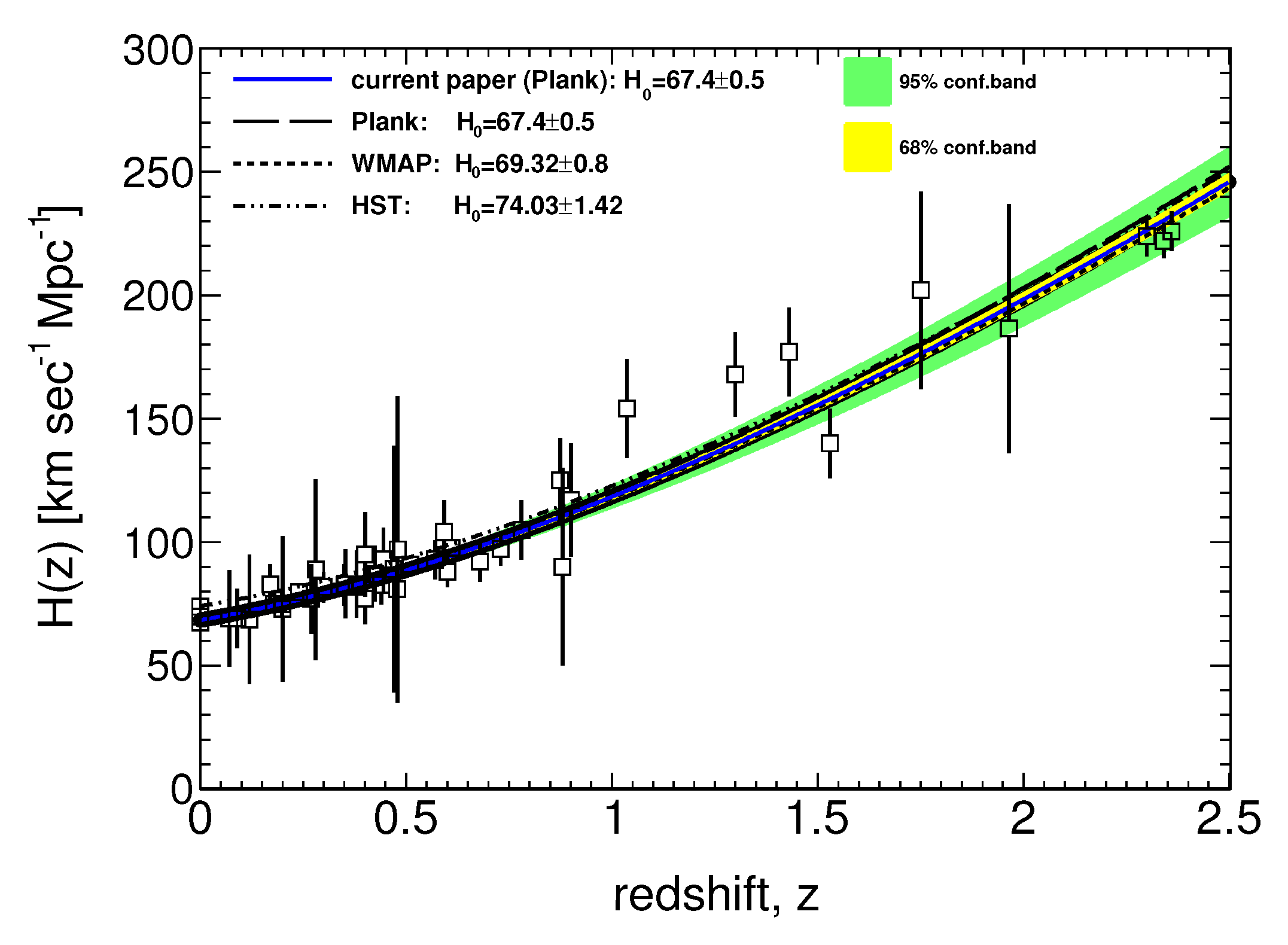
5. Preliminary Confrontation with Observations

We present here a first approach to using the model in detection of anisotropy. We obtained Hubble evolution from the Gemini Deep Survey (GDDS), Sloan Digital Sky Survey III Baryon Oscillation Spectroscopic Survey (SDSS-III), and highest redshift Lyα measurements. These data samples provide high-quality spectroscopy of red galaxies, some of which show stellar absorption features, indicating an old stellar population. The differential aging of these cosmic chronometers has been used to measure the observed Hubble parameter at different redshifts reported in Refs. [52,53,54,55], and does not include older results from earlier analyses of data subsets, or estimates that are no longer trusted to be reliable. Using the parameterised evolution
H ( z ) = H 0 Ω m 1 + z 3 + Ω Λ ,
confronted with our model Equation (47), for which we take the H 0 value from the Planck, WMAP, or HST evaluations, and Ω m and ϵ r are free parameters. This was done to study the effect of the assumed H 0 value on our results. By combining data sets taken from [52,53,54,55,56], a fit is done with the help of the Log-Likelihood and χ 2 methods implemented in the ROOT framework [57], for which the results on the anisotropy parameter are summarized in Table 1. The obtained Ω m from the fits were consistent with standard results and we did not estimate them worth indicating. This allows for plotting the Hubble diagrams shown in Figure 1. The differences in assumptions of the H 0 parameter do not noticeably affect the results (the lines overlap in Figure 1); however, as can be seen in Table 1, it does change the evaluation of the anisotropy parameter and its variance ϵ r ± σ , and somehow so does the regression method.
In Figure 1, the black lines (dashed, short-dashed, double dotted-dashed) represent the Hubble diagrams for the ΛCDM model fits with the fixed H 0 parameter with respect to the recent reports of the experimental collaborations, namely Plank [39], WMAP [58] and HST [42], while Ω m and ϵ r were released. The square data points with error bars are all taken from [52,53,54,55,56]. The colored line (solid blue) display our model using the H 0 determined from the Plank report [39]. The light yellow and green bands show its 1 and 2 σ confidence levels, respectively.
Our model matches within a 68% confidence level to the reference ΛCDM model, and thus is not significantly different from the isotropic case. This is reflected in Table 1, where the values of the anisotropy parameters, with their variances, are compatible with isotropy, except for the WMAP choice of H 0 combined either with the Log-Likelihood method or with the χ 2 and empty bins weighting method, where a slight detection is obtained. The weighting methods are recommended to be used in case of low statistics and when data represent counts with Poisson statistics. The χ 2 method without empty bins weighing results in very huge uncertainties for ϵ r . Except for the unweighted method, the large size of the variances should be noted. Therefore, clear detection would require cleaner data or larger sampling of the redshift range.
Although the level of uncertainties does not allow us to report definite values for ϵ r and these results are not giving clearly detectable anisotropy, we argue that the method could be used as a complement to the dipole/quadrupole approach from Ref. [59].

6. Conclusions

In this paper, we have constructed a Hubble law capable of being confronted with observations that were designed for an homogeneous and isotropic expanding universe, while allowing for global anisotropy in expansion. Such anisotropy would appear in observations designed without taking it into account as distortions of the redshift-distance behavior. This tool is obtained from solving the Einstein Field Equations for a Bianchi I model that is almost FLRW. For this model, the effect of anisotropy on redshift is obtained which is then synthesized for isotropy – assuming observation by an angle averaged redshift expression. We finally produce a Hubble function of redshift that we propose can be used in future confrontation with observations. Such a tool, we argue, is needed now as we have several reasons, starting from the back-reaction debate, and going on with some unexplained characteristics of the CMB that hint at the possibility that the role of anisotropy in the universe is not trivial. The model built in this paper discussed an anisotropic universe model that could be checked against CMB, or SNIa, predictions. As a preliminary example of how to use the model, we confronted it with three data sets and found no conclusive results. However, we argue that, with a more thorough approach, this method could be a useful complement to other approaches such as that of a Bolejko [59] late model measurement diagram. The model we build up will be checked in the next paper against cosmological data.

Author Contributions

All authors contributed equally. All authors have read and agreed to the published version of the manuscript.

Funding

Lanzhou University starting fund and the Fundamental Research Funds for the Central Universities (Grant No. lzujbky-2019-25).

Acknowledgments

MLeD acknowledges the financial support by the Lanzhou University starting fund and the Fundamental Research Funds for the Central Universities (Grant No. lzujbky-2019-25). M.D. thanks Xin Wu for his support in this research during the COVID-19 quarantine measures.

Conflicts of Interest

The authors declare no conflict of interest.

Appendix A. Solutions to Anisotropic Scale Parameters

Appendix A.1. Solutions with Ω0

From (13), one can integrate the anisotropic parameter, using (10) and the variable change X = a a 0 , into
ϵ = ϵ ˙ 0 H 0 Ω 0 a i a 0 a a 0 d X X 5 2 1 + Ω Λ Ω 0 X 3 .
We can further use the variable change
Z = Ω Λ Ω 0 X 3 X = Ω 0 Ω Λ Z 1 3 ,
d X = 1 3 Ω 0 Ω Λ 1 3 d Z Z 2 3 ,
to obtain in general
ϵ = ϵ ˙ 0 Ω Λ 3 H 0 Ω 0 Ω Λ Ω 0 a i a 0 3 Ω Λ Ω 0 a a 0 3 Z 1 2 1 1 + Z 1 2 1 d Z = ϵ ˙ 0 Ω Λ 3 H 0 Ω 0 2 1 + 1 Z Ω Λ Ω 0 a i a 0 3 Ω Λ Ω 0 a a 0 3 = 2 ϵ ˙ 0 3 H 0 Ω 0 Ω 0 a i a 0 3 + Ω Λ Ω 0 a a 0 3 + Ω Λ ,
so we can build the ratio ( Ω Λ = 1 Ω 0 )
ϵ r ϵ 0 = Ω 0 a i a 0 3 + Ω Λ Ω 0 a r a 0 3 + Ω Λ Ω 0 a i a 0 3 + Ω Λ 1 .

Appendix A.2. Solutions with Ωm

Using Ω Λ = 1 Ω 0 and defining x with Ω 0 = Ω m 2 3 H 0 ϵ ˙ 0 1 + ϵ 0 = Ω m x , so ϵ ˙ 0 H 0 = 3 2 1 + ϵ 0 x , we can rewrite Equation (A4), at present time
ϵ 0 = 3 1 + ϵ 0 x Ω m x 1 Ω m + x + Ω m x a i a 0 3 1 .
Assuming that x Ω m , we linearize the above expression in x. We first linearize all factors
ϵ 0 3 1 + ϵ 0 Ω m x Ω m a i a 0 3 1 + 1 1 × 1 + 1 Ω m a i a 0 3 1 2 Ω m a i a 0 3 1 + 1 Ω m a i a 0 3 1 + 1 x + O ( x 2 ) ,
to finally simplify the linearization and retain only the linear terms
ϵ 0 3 1 + ϵ 0 Ω m Ω m a i a 0 3 1 + 1 1 x .
Finally, solving for x, we find the expression of the derivative in the constant of integration in terms of the present anisotropic perturbation parameter and define the constant Δ 0
ϵ ˙ 0 H 0 = 3 2 1 + ϵ 0 x ϵ 0 / 2 Ω m Ω m a i a 0 3 1 + 1 1 = ϵ 0 Δ 0
with Δ 0 = 2 Ω m Ω m a i a 0 3 1 + 1 1 .

Appendix B. Anisotropic Redshift Hubble Calculations

Appendix B.1. Anisotropic Redshift Terms

Applying Equation (29) to introduce the redshift relation to the scale factors, we have the following:
a 0 a = 1 + z 1 + 1 + ϵ 2 ϵ 1 + 1 + ϵ 0 2 ϵ 0 .
From above, we can also compose
a 0 a 2 1 1 + ϵ = 1 + z 2 1 + ϵ 2 2 1 + ϵ 1 + 1 + ϵ 0 2 ϵ 0 ,
a 0 a 2 1 + ϵ 0 1 + ϵ = 1 + z 2 1 + ϵ 2 2 1 + ϵ 1 + ϵ 0 2 2 1 + ϵ 0 .
Introducing, with Equation (13), the anisotropic perturbation parameter’s derivative, and applying the expressions above, we can rewrite with redshift some of the factors present in Equation (36)
ϵ ˙ 3 1 + ϵ = ϵ ˙ 0 3 1 + z 3 ×
1 + ϵ 2 2 1 + ϵ 1 + 1 + ϵ 0 2 ϵ 0 1 + 1 + ϵ 2 ϵ 1 + 1 + ϵ 0 2 ϵ 0 ,
a a 0 3 = 1 + z 3 1 + 1 + ϵ 2 ϵ 1 + 1 + ϵ 0 2 ϵ 0 3 ,
a 0 a 3 1 + ϵ 0 1 + ϵ = 1 + z 3 1 + ϵ 2 2 1 + ϵ 1 + ϵ 0 2 2 1 + ϵ 0 1 + 1 + ϵ 2 ϵ 1 + 1 + ϵ 0 2 ϵ 0 .
They can then be linearized in ϵ as
ϵ ˙ 3 1 + ϵ ϵ ˙ 0 3 1 + z 3 1 + ϵ 0 2 ϵ ϵ 0 3 ,
a a 0 3 1 + z 3 1 3 2 ϵ 0 ϵ ϵ 0 1 1 + z 3 ,
a 0 a 3 1 + ϵ 0 1 + ϵ 1 + z 3 1 + ϵ 0 2 ϵ ϵ 0 1 .

Appendix B.2. Anisotropic Hubble Parameter

The Hubble parameter (36), joined to the expressions above, also using Equation (A8), then reads, to linear order
H ϵ ˙ 0 3 2 1 + z 6 1 + ϵ 0 ϵ ϵ 0 3 + H 0 2 Ω m 1 + z 3 1 + ϵ 0 2 ϵ ϵ 0 1 1 + 1 + 2 3 H 0 ϵ ˙ 0 1 + ϵ 0 H 0 ϵ 0 3 Δ 0 2 1 + z 6 1 + ϵ 0 ϵ ϵ 0 3 + Ω m 1 + z 3 1 + ϵ 0 2 ϵ ϵ 0 1 1 + 1 + 2 3 ϵ 0 Δ 0
and is further reduced to linear order as
H H 0 Ω m 1 + z 3 1 + ϵ 0 2 ϵ ϵ 0 1 1 + 1 + 2 3 ϵ 0 Δ 0
with Δ 0 = 2 Ω m Ω m a i a 0 3 1 + 1 1 .
From Equation (A4), in the general case, we get
ϵ = 2 ϵ ˙ 0 H 0 Ω m x 1 Ω m + x + Ω m x a i a 0 3 1 Ω m + x + Ω m x a a 0 3 .
Then, employing Equation (A8), as in the derivation from Appendix A, we linearize in x
ϵ ϵ 0 Δ 0 2 Ω m Ω m a i a 0 3 1 + 1 a a 0 3 2 a a 0 3 Ω m a a 0 3 1 + 1 + a a 0 3 1 2 Ω m a a 0 3 1 + 1 a i a 0 3 1 2 Ω m a i a 0 3 1 + 1 + 1 Ω m x + O ( x 2 ) .
Finally, introducing redshift with Equation (A17) and the definition (A20), we can obtain the linear form for ϵ :
ϵ ϵ 0 Ω m 1 + z i 3 1 + 1 1 Ω m 1 + z i 3 1 + 1 Ω m 1 + z 3 1 + 1
ϵ 0 1 Ω m 1 + z 3 1 + 1 Ω m 1 + z i 3 1 + 1 1 1 Ω m 1 + z i 3 1 + 1 ,
from which we deduce the ratio
ϵ ϵ 0 1 Ω m 1 + z 3 1 + 1 Ω m 1 + z i 3 1 + 1 1 1 Ω m 1 + z i 3 1 + 1 ,
We can then use the scale-redshift approximation (A17) and the values at recombination to express
a i a 0 3 1 + z i 3 = 10 3 n + 3
ϵ 0 Ω m 10 3 n + 3 1 + 1 1 ϵ r Ω m 10 3 n + 3 1 + 1 Ω m 10 9 1 + 1 , ϵ Ω m 10 3 n + 3 1 + 1 Ω m 1 + z 3 1 + 1 ϵ r Ω m 10 3 n + 3 1 + 1 Ω m 10 9 1 + 1 ,
(where the relevant input measurements are ϵ r 10 5 for a r a 0 = 10 3 and n = log 10 a r a i ) to input in Equation (A19) and finally get the Hubble redshift relation
H H 0 Ω m 1 + z 3 1 + ϵ r 2 1 I z I 0 I z r 1 + 1 + 2 Ω m 3 1 Ω m ϵ 0 I 0 ,
+ 1 + Ω m 3 ϵ r I 0 I z r ¯ ,
with I 0 = Ω m 10 3 n + 3 1 + 1 ,
I z r = Ω m 10 9 1 + 1 ,
and I z = Ω m 1 + z 3 1 + 1 .

References

  1. Rasanen, S. Dark energy from back-reaction. J. Cosmol. Astropart. Phys. 2004, 2, 3. [Google Scholar] [CrossRef] [Green Version]
  2. Rasanen, S. Accelerated expansion from structure formation. J. Cosmol. Astropart. Phys. 2006, 11, 3. [Google Scholar] [CrossRef] [Green Version]
  3. Marozzi, G.; Uzan, J.P. Late time anisotropy as an imprint of cosmological backreaction. Phys. Rev. D 2012, 86, 063528. [Google Scholar] [CrossRef] [Green Version]
  4. Flanagan, E.E. Can superhorizon perturbations drive the acceleration of the universe? Phys. Rev. D 2005, 71, 103521. [Google Scholar] [CrossRef] [Green Version]
  5. Misner, C.W. The isotropy of the universe. Astrophys. J. 1968, 151, 431. [Google Scholar] [CrossRef]
  6. Gibbons, G.W.; Hawking, S.W. Action integrals and partition functions in quantum gravity. Phys. Rev. D 1977, 15, 2752. [Google Scholar] [CrossRef]
  7. Penzias, A.A.; Wilson, R.W. A measurement of excess antenna temperature at 4080 Mc/s. Astrophys. J. 1965, 142, 419. [Google Scholar] [CrossRef]
  8. Dicke, R.H.; Peebles, P.J.E.; Roll, P.G.; Wilkinson, D.T. Cosmic Black-Body Radiation. Astrophys. J. 1965, 142, 414. [Google Scholar] [CrossRef]
  9. Stoeger, S.J.; Araujo, W.R.M.; Gebbie, T. The limits on cosmological anisotropies and inhomogeneities from COBE data. Astrophys. J. 1997, 476, 435. [Google Scholar] [CrossRef] [Green Version]
  10. Maartens, R.; Ellis, G.F.R.; Stoeger, W.R. Limits on anisotropy and inhomogeneity from the cosmic background radiation. Phys. Rev. D 1995, 51, 1525. [Google Scholar] [CrossRef] [Green Version]
  11. Maartens, R.; Ellis, G.F.R.; Stoeger, W.R. Improved limits on anisotropy and inhomogeneity from the cosmic background radiation. Phys. Rev. D 1995, 51, 5942. [Google Scholar] [CrossRef] [PubMed]
  12. Friedman, A. On space curvature. Z. Phys. 1992, 10, 377. [Google Scholar] [CrossRef]
  13. Lemaitre, G. Expansion of the universe, The expanding universe. Mon. Not. R. Astron. Soc. 1931, 91, 490. [Google Scholar] [CrossRef] [Green Version]
  14. Robertson, H.P. Relativistic cosmology. Rev. Mod. Phys. 1933, 5, 62. [Google Scholar] [CrossRef]
  15. Walker, A.G. Distance in an expanding universe. Mon. Not. R. Astron. Soc. 1933, 94, 159. [Google Scholar] [CrossRef] [Green Version]
  16. Collins, C.B.; Hawking, S.W. The rotation and distortion of the universe. Mon. Not. R. Astron. Soc. 1973, 162, 307. [Google Scholar] [CrossRef]
  17. Mather, J.C.; Cheng, E.S.; Eplee, R.E., Jr.; Isaacman, R.B.; Meyer, S.S.; Shafer, R.A.; Weiss, R.; Wright, E.L.; Bennett, C.L.; Boggess, N.W.; et al. A preliminary measurement of the cosmic microwave background spectrum by the Cosmic Background Explorer (COBE) satellite. Astrophys. J. 1990, 354, L37–L40. [Google Scholar] [CrossRef]
  18. Bennett, C.L.; Bay, M.; Halpern, M.; Hinshaw, G.; Jackson, C.; Jarosik, N.; Kogut, A.; Limon, M.; Meyer, S.S.; Page, L.; et al. The Microwave Anisotropy Probe Mission. Astrophys. J. 2003, 583, 1–23. [Google Scholar] [CrossRef] [Green Version]
  19. Team, P.H.C.; Ade, P.A.R.; Aghanim, N.; Ansari, R.; Arnaud, M.; Ashdown, M.; Aumont, J.; Banday, A.J.; Bartelmann, M.; Bartlett, J.G.; et al. Planck early results. IV. First, assessment of the High Frequency Instrument in-flight performance. Astron. Astrophys. 2011, 536, A4. [Google Scholar] [CrossRef]
  20. Eriksen, H.K.; Hansen, F.K.; Banday, A.J.; Gorski, K.M.; Lilje, P.B. Asymmetries in the Cosmic Microwave Background anisotropy field. Astrophys. J. 2004, 605, 14. [Google Scholar] [CrossRef]
  21. Hansen, F.K.; Banday, A.J.; Gorski, K.M. Testing the cosmological principle of isotropy: Local power-spectrum estimates of the WMAP data. Mon. Not. R. Astron. Soc. 2004, 354, 641. [Google Scholar] [CrossRef] [Green Version]
  22. Jaffe, T.R.; Banday, A.J.; Eriksen, H.K.; Gorski, K.M.; Hansen, F.K. Evidence of vorticity and shear at large angular scales in the WMAP data: A violation of cosmological isotropy? Astrophys. J. 2005, 629, L1. [Google Scholar] [CrossRef]
  23. Hoftuft, J.; Eriksen, H.K.; Banday, A.J.; Gorski, K.M.; Hansen, F.K.; Lilje, P.B. Increasing evidence for hemispherical power asymmetry in the five-year WMAP data. Astrophys. J. 2009, 699, 985. [Google Scholar] [CrossRef] [Green Version]
  24. Ade, P.A.R.; Aghanim, N.; Armitage-Caplan, C.; Arnaud, M.; Ashdown, M.; Atrio-Barandela, F.; Aumont, J.; Baccigalupi, C.; Banday, A.J.; Barreiro, R.B.; et al. Planck2013 results. XXIII. Isotropy and statistics of the CMB. Astron. Astrophys. 2014, 571, A23. [Google Scholar] [CrossRef] [Green Version]
  25. Akrami, Y.; Fantaye, Y.; Shafieloo, A.; Eriksen, H.K.; Hansen, F.K.; Banday, A.J.; Górski, K.M. Power asymmetry in WMAP and Planck temperature sky maps as measured by a local variance estimator. Astrophys. J. 2014, 784, L42. [Google Scholar] [CrossRef] [Green Version]
  26. Zhao, W.; Santos, L. The Weird Side of the Universe: Preferred Axis. In Proceedings of the 7th International Workshop on Astronomy and Relativistic Astrophysics (IWARA 2016), International Journal of Modern Physics: Conference Series, Gramado, Brazil, 9–13 October 2016; Volume 45, p. 1760009. [Google Scholar] [CrossRef] [Green Version]
  27. Contreras, D.; Hutchinson, J.; Moss, A.; Scott, D.; Zibin, J.P. Closing in on the large-scale CMB power asymmetry. Phys. Rev. D 2018, 97, 063504. [Google Scholar] [CrossRef] [Green Version]
  28. O’Dwyer, M.; Copi, C.J.; Nagy, J.M.; Netterfield, C.B.; Ruhl, J.; Starkman, G.D. Hemispherical Variance Anomaly and Reionization Optical Depth. arXiv 2019, arXiv:1912.02376. [Google Scholar]
  29. Schwarz, D.J.; Starkman, G.D.; Huterer, D.; Copi, C.J. Is the low-l microwave background cosmic? Phys. Rev. Lett. 2004, 93, 221301. [Google Scholar] [CrossRef] [Green Version]
  30. Copi, C.J.; Huterer, D.; Schwarz, D.J.; Starkman, G.D. On the large-angle anomalies of the microwave sky. Mon. Not. R. Astron. Soc. 2006, 367, 79. [Google Scholar] [CrossRef] [Green Version]
  31. Copi, C.; Huterer, D.; Schwarz, D.; Starkman, G. Uncorrelated universe: Statistical anisotropy and the vanishing angular correlation function in WMAP years 1–3. Phys. Rev. D 2007, 75, 023507. [Google Scholar] [CrossRef] [Green Version]
  32. Copi, C.J.; Huterer, D.; Schwarz, D.J.; Starkman, G.D. Large-angle anomalies in the CMB. Adv. Astron. 2010, 2010, 847541. [Google Scholar] [CrossRef]
  33. Copi, C.J.; Huterer, D.; Schwarz, D.J.; Starkman, G.D. Large-scale alignments from WMAP and Planck. Mon. Not. R. Astron. Soc. 2015, 449, 3458. [Google Scholar] [CrossRef] [Green Version]
  34. Marcos-Caballero, A.; Martínez-González, E. Scale-dependent dipolar modulation and the quadrupole-octopole alignment in the CMB temperature. J. Cosmol. Astropart. Phys. 2019, 1910, 53. [Google Scholar] [CrossRef] [Green Version]
  35. Cruz, M.; Martinez-Gonzalez, E.; Vielva, P.; Cayon, L. Detection of a non-Gaussian spot in WMAP. Mon. Not. R. Astron. Soc. 2005, 356, 29. [Google Scholar] [CrossRef]
  36. Cruz, M.; Cayon, L.; Martinez-Gonzalez, E.; Vielva, P.; Jin, J. The non-gaussian cold spot in the 3 year Wilkinson microwave anisotropy probe data. Astrophys. J. 2007, 655, 11. [Google Scholar] [CrossRef]
  37. Cruz, M.; Tucci, M.; Martinez-Gonzalez, E.; Vielva, P. The non-Gaussian cold spot in Wilkinson Microwave Anisotropy Probe: Significance, morphology and foreground contribution. Mon. Not. R. Astron. Soc. 2006, 369, 57. [Google Scholar] [CrossRef] [Green Version]
  38. Bolejko, K. Emerging spatial curvature can resolve the tension between high-redshift CMB and low-redshift distance ladder measurements of the Hubble constant. Phys. Rev. D 2018, 97, 103529. [Google Scholar] [CrossRef] [Green Version]
  39. Planck; Aghanim, N.; Akrami, Y.; Ashdown, M.; Aumont, J.; Baccigalupi, C.; Ballardini, M.; Banday, A.J.; Barreiro, R.B.; Bartolo, N.; et al. Planck 2018 results. VI. Cosmological parameters. arXiv 2018, arXiv:1807.06209. [Google Scholar]
  40. Riess, A.G.; Casertano, S.; Yuan, W.; Macri, L.; Anderson, J.; MacKenty, J.W.; Bowers, J.B.; Clubb, K.I.; Filippenko, A.V.; Jones, D.O.; et al. New Parallaxes of Galactic Cepheids from Spatially Scanning theHubble Space Telescope: Implications for the Hubble Constant. Astrophys. J. 2018, 855, 136. [Google Scholar] [CrossRef] [Green Version]
  41. Riess, A.G.; Casertano, S.; Yuan, W.; Macri, L.; Bucciarelli, B.; Lattanzi, M.G.; MacKenty, J.W.; Bowers, J.B.; Zheng, W.; Filippenko, A.V.; et al. Milky Way Cepheid Standards for Measuring Cosmic Distances and Application to Gaia DR2: Implications for the Hubble Constant. Astrophys. J. 2018, 861, 126. [Google Scholar] [CrossRef]
  42. Riess, A.G.; Casertano, S.; Yuan, W.; Macri, L.M.; Scolnic, D. Large Magellanic Cloud Cepheid standards provide a 1% foundation for the determination of the Hubble constant and stronger evidence for physics beyond ΛCDM. Astrophys. J. 2019, 876, 85. [Google Scholar] [CrossRef]
  43. Bennett, C.L.; Hill, R.S.; Hinshaw, G.; Larson, D.; Smith, K.M.; Dunkley, J.; Gold, B.; Halpern, M.; Jarosik, N.; Kogut, A.; et al. Seven-year wilkinson microwave anisotropy probe (WMAP*) observations: Are there cosmic microwave background anomalies? Astrophys. J. Suppl. 2011, 192, 17. [Google Scholar] [CrossRef] [Green Version]
  44. Rameez, M.; Sarkar, S. Is there really a Hubble tension? arXiv 2019, arXiv:1911.06456. [Google Scholar]
  45. Pontzen, A.; Challinor, A. Bianchi model CMB polarization and its implications for CMB anomalies. Mon. Not. R. Astron. Soc. 2007, 380, 1387. [Google Scholar] [CrossRef] [Green Version]
  46. Sung, R.; Short, J.; Coles, P. Statistical characterization of cosmic microwave background temperature patterns in anisotropic cosmologies. Mon. Not. R. Astron. Soc. 2011, 412, 492–502. [Google Scholar] [CrossRef] [Green Version]
  47. Russell, E.; Kılınc, C.B.; Pashaev, O.K. Bianchi I model: An alternative way to model the present-day Universe. Mon. Not. R. Astron. Soc. 2014, 442, 2331–2341. [Google Scholar] [CrossRef] [Green Version]
  48. Macpherson, H.J. Inhomogeneous Cosmology in an Anisotropic Universe. Ph.D. Thesis, Monash University, Clayton, Australia, 2019. [Google Scholar]
  49. Cea, P. Eur. Confronting the ellipsoidal universe to the Planck 2018 data. Phys. J. Plus 2020, 135, 150. [Google Scholar] [CrossRef]
  50. Jacobs, K.C. Bianchi Type I Cosmological Models. Ph.D. Thesis, Caltech University, Pasadena, CA, USA, 1968. [Google Scholar]
  51. Smoot, G.F.; Bennett, C.L.; Kogut, A.; Wright, E.L.; Aymon, J.; Boggess, N.W.; Cheng, E.S.; De Amici, G.; Gulkis, S.; Hauser, M.; et al. Structure in the COBE differential microwave radiometer first-year maps. Astrophys. J. 1992, 396, L1. [Google Scholar] [CrossRef]
  52. Simon, J.; Verde, L.; Jimenez, R. Constraints on the redshift dependence of the dark energy potential. Phys. Rev. D 2005, 71, 123001. [Google Scholar] [CrossRef] [Green Version]
  53. Moresco, M.; Cimatti, A.; Jimenez, R.; Pozzetti, L.; Zamorani, G.; Bolzonella, M.; Dunlopd, J.; Lamareillee, F.; Mignolic, M.; Pearced, H.; et al. Improved constraints on the expansion rate of the Universe up to z 1.1 from the spectroscopic evolution of cosmic chronometers. J. Cosmol. Astropart. Phys. 2012, 8, 6. [Google Scholar] [CrossRef] [Green Version]
  54. Anderson, L.; Aubourg, E.; Bailey, S.; Beutler, F.; Bolton, A.S.; Brinkmann, J.; Brownstein, J.R.; Chuang, C.-H.; Cuesta, A.J.; Dawson, K.S.; et al. The clustering of galaxies in the SDSS-III Baryon Oscillation Spectroscopic Survey: Measuring DA and H at z = 0.57 from the baryon acoustic peak in the Data Release 9 spectroscopic Galaxy sample. Mon. Not. R. Astron. Soc. 2014, 439, 83. [Google Scholar] [CrossRef] [Green Version]
  55. Yu, H.; Ratra, B.; Wang, F.-Y. Hubble parameter and Baryon Acoustic Oscillation measurement constraints on the Hubble constant, the deviation from the spatially flat ΛCDM model, the deceleration-acceleration transition redshift, and spatial curvature. Astrophys. J. 2018, 856, 3. [Google Scholar] [CrossRef] [Green Version]
  56. Sharov, G.; Vorontsova, E. Parameters of cosmological models and recent astronomical observations. J. Cosmol. Astropart. Phys. 2014, 10, 57. [Google Scholar] [CrossRef] [Green Version]
  57. Antcheva, I.; Ballintijn, M.; Bellenot, B.; Biskup, M.; Brun, R.; Buncic, N.; Canal, P.; Casadei, D.; Couet, O.; Fine, V.; et al. ROOT—A C++ framework for petabyte data storage, statistical analysis and visualization. Comput. Phys. Commun. 2009, 180, 2499. [Google Scholar] [CrossRef] [Green Version]
  58. Komatsu, E.; Smith, K.M.; Dunkley, J.; Bennett, C.L.; Gold, B.; Hinshaw, G.; Jarosik, N.; Larson, D.; Nolta, M.R.; Page, L.; et al. Seven-year Wilkinson microwave anisotropy probe (WMAP) observations: Cosmological interpretation. Astrophys. J. Suppl. 2011, 192. [Google Scholar] [CrossRef] [Green Version]
  59. Bolejko, K.; Nazer, M.A.; Wiltshire, D.L. Differential cosmic expansion and the Hubble flow anisotropy. J. Cosmol. Astropart. Phys. 2016, 6, 35. [Google Scholar] [CrossRef] [Green Version]
Figure 1. Hubble diagram confrontation of ΛCDM and our model Equation (47) assuming that H 0 was taken from the Planck, WMAP, and HST results.
Symmetry 12 01741 g001
Table 1. Model parameters analysis to obtain ϵ r ± σ . We fit the data from [52,53,54,55,56] with two different methods, namely Log-Likelihood and χ 2 . In addition to fit method, there are two weighting methods for the fitted distribution. The designation “weighting empty bins” means that we assign weights equal to unity to all bins, including empty bins, while the method without weighting does not use any assumption about the data-points weights. In all fits, we fixed the H 0 value and release Ω M and ϵ r parameters using Equation (47). The fixed H 0 refers to the reports from the different experimental collaboration, namely Plank [39], WMAP [58], and HST [42].
Fit MethodPlankWMAPHST
ϵ r σ ϵ r σ ϵ r σ
Log-Likelihood (with/without weighting empty bins)0.250.370.130.120.250.37
χ 2 (without weighting empty bins)0.131.320.254.030.131..31
χ 2 (with weighting empty bins)0.250.370.130.120.250.37
Publisher’s Note: MDPI stays neutral with regard to jurisdictional claims in published maps and institutional affiliations.

