Article

On the Statistical GARCH Model for Managing the Risk by Employing a Fat-Tailed Distribution in Finance

1
Division of Computational Mathematics and Engineering, Institute for Computational Science, Ton Duc Thang University, Ho Chi Minh City 70000, Vietnam
2
Faculty of Mathematics and Statistics, Ton Duc Thang University, Ho Chi Minh City 70000, Vietnam
3
Department of Mathematics, College of Science, King Saud University, P.O. Box 2455, Riyadh 11451, Saudi Arabia
4
AMPSAS, University College Dublin, 4 Dublin, Ireland
5
Institute of Space Sciences, 077125 Magurele-Bucharest, Romania
6
Department of Mathematics, Cankaya University, 06530 Balgat, Ankara, Turkey
*
Author to whom correspondence should be addressed.
Symmetry 2020, 12(10), 1698; https://doi.org/10.3390/sym12101698
Submission received: 7 September 2020 / Revised: 8 October 2020 / Accepted: 10 October 2020 / Published: 15 October 2020

Abstract

:
The Conditional Value-at-Risk (CVaR) is a coherent measure that evaluates the risk for different investing scenarios. On the other hand, since the extreme value distribution has been revealed to furnish better financial and economical data adjustment in contrast to the well-known normal distribution, we here employ this distribution in investigating explicit formulas for the two common risk measures, i.e., VaR and CVaR, to have better tools in risk management. The formulas are then employed under the generalized autoregressive conditional heteroskedasticity (GARCH) model for risk management as our main contribution. To confirm the theoretical discussions of this work, the daily returns of several stocks are considered and worked out. The simulation results uphold the superiority of our findings.
MSC:
60G70; 91B30; 62M10
JEL Classification:
G32; C53

1. Introduction

1.1. Literature Review on VaR and CVaR

According to the branch of application at which the concept of risk is situated, risk can be defined and expressed in several ways each has its own target (Reference [1], Chapters 14–15).
As given in the well-known Basel Committee on Banking Supervision (BCBS), a finance institute is forced to fulfill capital needs to cover all possible losses because of risk sources during normal operations: i.e., operational risk, market risk and credit risk [2]. A finance firm may need to figure out possible losses to its portfolios so as to better allocate its funds and plan for payments to investors, see also the discussions in Reference [3].
In the field of mathematical finance, one of the pioneer measures for doing such a thing is the Value-at-Risk (VaR). VaR was first given by Markowitz in Reference [4] and Roy in Reference [5] separately to estimate the portfolio’s VaR and actually for optimizing profit for the associated specific risk levels. This measure is defined as follows [6]:
VaR α ( X ) : = min { z R | F X ( z ) α } ,
wherein X is a random variable, α is the pre-determined tail level, F X ( · ) stands for the cumulative distribution function (CDF), and the function min is sometimes replaced by inf. Note that both cases of lower tails or losses (e.g., α equal to 1%) or upper tails or profits (e.g., α equal to 99%) can be used by (1) when employing α or 1 α as tail levels. However, in this work we focus on profits, though everything is exchangeable.
The approaches to VaR could be investigated in three categories [7]: (i) fully parametric models approach based on a volatility models; (ii) non-parametric approaches based on the Historical Simulation (HS) methods and (iii) Extreme Value Theory approach based on modeling the tails of the return distribution. It is known that VaR is used for obtaining the loss in the entity being evaluated and the occurrence probability for the loss defined. The VaR measure is normally employed at the institutional portfolios by banks to understand the occurrence and extent ratio of possible losses [8]. Note also that a fundamental factor in optimization of a portfolio is to find a right measure of risk to scalarize the portfolio’s risk.
On the other hand, as long as an investment has given an (almost) stable behavior along time, then the VaR can be enough for the management of risk in the portfolio including the investment [9]. Nonetheless, by losing the stability, the chance that this risk measure gives a full picture of involved risks gets decreased since it is not that sensitive to anything after its own boundary (threshold). To illustrate further, lately as an instance, the oil sector has reflected instability in international oil prices, which have been more representative since 2004 and respond to various existing factors.
Conditional Value at Risk (CVaR), which is also sometimes called the AVaR, or expected tail loss (ETL), is actually the average loss of the specified distribution in the extreme tail area [10]. Hence, it is an alternative measure of risk which could overcome on some of the drawbacks of VaR and always yields a higher magnitude for the risk in contrast to the VaR (Reference [1], chapter 15). The mechanism of CVaR is based on the conditional expectation of the loss that exceeds VaR, viz,
CVaR α ( X ) : = E X | X VaR α ( X ) .
CVaR is constructed from the VaR for a portfolio or investment and is employed in the optimization of a portfolio for efficient risk allocation. Risk allocation is the process of identifying risk and determining how and to what extent they should be shared. Most owners understand that risk is an inherent part of the construction process and cannot be eliminated. Accurate risk identification and the assignment of risk to the party make the stock-holders or financial managers to carefully step ahead and minimize the risk of losing the capital. This could improve quality, reduce delays and resolve disputes efficiently [11].
The definition (2) is also called the lower CVaR (Tail VaR) as long as the inequality in the conditional expectation is with equality. But once the inequality be strict (without the equality sign), it will be called the upper CVaR definition (or expected shortfall (ES)) [12]. Some stock markets, such as NYSE, have required their accepted companies to estimate and report their risk employing ES, which makes this measure an important and useful risk measure.
Another definition of CVaR for continuous probability distributions is [13]:
CVaR α ( X ) : = z d F X α ( z ) ,
wherein the α -tail distribution is defined by
F X α ( z ) = 0 , z < VaR α ( X ) , F X ( z ) α 1 α , z VaR α ( X ) .
By considering the examined time horizon (yearly, monthly, weekly, or even daily), VaR could be computed showing the suffering probability for a loss while the mixture of a specific investment portfolio is given. Although this is a simple and widely-used measure for financial traders and managers, it has its own limitations which restricts its application and reliably in many of the practical cases. Some of these such downfalls are discontinuity for some discrete distributions, lack of convexity, and, mainly, its inability to quantify risk in the extreme tail region after the boundary of VaR. And because of this, CVaR was introduced. In the recent document published by the Basel Committee on Banking Supervision in Reference [14], both the value-at-risk and the expected shortfall have been considered and discussed in detail.
Another limitation in risk allocation and managing portfolios is the assumption of normal distribution for the underlying factors. Anyhow, it was revealed that the normal assumption is not the best consideration for finance instruments, yielding in the application of alternative distributions. Now, by encountering a volatile and uncertain scenario, the question is how we could find efficient models that facilitate better risk management?
This paper discusses closed and explicit formulations for the measures VaR and CVaR under the extreme value distribution (EVD). This is important since history has revealed that millions of dollars may be lost in a short piece of time because of failure in handling the financial risks in market. Within this circumstance, we will concentrate this paper on VaR and CVaR explicit formulations, comparing the precision of both values and taking into account the EVD as an alternative to the well-known normal distribution for risk management. To support the discussions, the contribution of this work as an application is considered and simulated from time series in forecasting the prices/returns of several well-known stocks in different period of times under the generalized autoregressive conditional heteroskedasticity (GARCH) model [15].

1.2. Garch Model

Several works (see Reference [16] and the references cited therein) have revealed that the future variance prediction through modern GARCH-type models is necessary for managing portfolio risk efficiently, due to the presence of the effects of heteroskedastic (i.e., the volatility of the under studying process is basically not constant.)
It is known that the volatility is the square root of the conditional variance of the log return process given its previous values using F t 1 as the σ -algebra generated by x 0 , x 1 , , x t 1 . This means, as long as p t (price of a stock in stick exchange at time t) is the time series computed at time t, we can then define the log returns as follows [17]:
x t = log p t log p t 1 ,
and then we can also define
σ t 2 = Var [ x t 2 | F t 1 ] .
Since we will illustrate the usefulness of the proposed explicit risk measures under the EVD by the GARCH model, it is now requisite to recall the GARCH model, which is in fact an autoregressive moving average model (ARMA) model for the variance of error [17]. Among the general parametric case of GARCH(p,q) process at which p is the order of the GARCH terms σ 2 ; and q is the order of the ARCH terms ϵ 2 , we here use the GARCH(1,1) as follows:
r t = ϱ + ε t = ϱ + σ t z t , σ t 2 = w + λ ε t 1 2 + β σ t 1 2 ,
wherein z t is a stochastic piece (independent and identically distributed (i.i.d.) innovations having unit variance and vanishing mean). Here, w > 0 , r t is the actual return, ϱ is the expected return, σ t is the volatility of the returns on day t, and finally
λ 0 , β 0 , λ + β < 1 .
The condition λ + β < 1 in (8) shows to have a stationary solution of the GARCH model.
The model (7) has become employed in economic time series modeling and is programmed in several of the econometric and statistics packages [18]. It is favored over other models of stochastic volatility (SV) by many practitioners due to its straightforward programming. Since it is in fact given by stochastic difference equations in discrete time, the likelihood function is easier to tackle than models with continuous-time feature, and also because finance information is basically given at discrete intervals [19]. To see some background on the relation between the GARCH-EVT model and the GARCH-VaR or GARCH-CVaR, one may refer to Reference [20].
A fruitful feature of the GARCH-type models is that they capture the fat-tailedness along with volatility clustering. Following the result in Reference [21], the stationary solution of GARCH(1,1) process follows a heavy-tailed distribution. Therefore, the GARCH-type models turn to be an effective instrument in risk management.

1.3. Motivation and Article’S Plan

The motivation behind choosing the EVD for risk management does not only lie in the fact that no closed form measures for this distribution are existed in literature, but also in the point that it has fatter right tail in contrast to the commonly used normal distribution [22]. It must be noticed that the selection of distribution for computing VaR and CVaR impacts the approximation of the quartiles that determine the risk. Besides, better adjustment of the empirical data to a specific distribution type enables construction of functions that more efficiently estimate the risk provided the conditions of volatility and uncertainty.
It is necessary to state that very recently Norton et al. in Reference [23] investigated the CVaR for some common distributions and more specifically derived a generic expression for GEV distribution, at which this paper deals with a special case of 0 as the free parameter. Here, the way of deriving the closed formulation for the VaR and CVaR under the EVD is different and mainly we then focus to employ the obtained VaR/CVaR formulas to the historical returns of several U.S. stocks using the GARCH process. Furthermore, the methodology of this work follows the footsteps of the discussions of [24], but somewhat different since neither no closed forms for VaR and CVaR under EVD is given nor a direct application on the GARCH process is given in Reference [24] for forecasting the risk on the tickers considered in this paper. For more, an interested reader may refer to Reference [25].
The remaining sections of this work are organized in what follows. Section 2 is devoted to the basic notions of the EVD and obtaining a closed formulation for the VaR measure under this distribution. Distribution of the innovations plays a key role when analyzing unconditional and conditional downside risk. Next, in Section 3, the CVaR is given. Then, Section 4 provides an application of the new closed formulations for computing the VaR and CVaR risk measures in a portfolio having a stock based on the GARCH(1,1) process; one may refer to Reference [26] for further discussions on this. In time series for finance and economy, specific characteristics, like the volatility clustering and being fat-tailed, yield challenges in handling downside risk evaluation. However, the model (7) captures such characteristics regardless of the distributional assumptions on the innovation process. The paper ends, in Section 5, by providing several comments and outlooks for future works.

2. VaR Based on the EVD

The EVD is fruitful in forecasting when there is a heavier right tail on the underlying prices in market and to describe extremely unlikely events [27]. The EVD with real parameters μ as the location parameter and σ as the scale parameter presents a statistical continuous distribution given over the set of real numbers. An important point in the field of extreme value theory (EVT) is that the EVD is broadly employed to express situations that are extremely unlikely (i.e., those at which datasets include variates with extreme deviations from the median), for instance, in catastrophic insurance losses and risk management in portfolio.
Here, when
X EVD ( μ , σ ) ,
then the probability density function (PDF) of this distribution is defined by:
f ( x ) = e μ x σ e μ x σ σ .
Its CDF is given by
F ( x ) = e e μ x σ .
While the overall behavior of the probability density function (PDF) of the EVD is smooth and uni-modal, the parameters μ and σ determine the horizontal location and overall height and steepness, respectively, of the PDF. Furthermore, the important moments for this distribution can be written as follows:
Mean ( X ) = μ + γ σ ,
Median ( X ) = μ σ log ( log ( 2 ) ) ,
Variance ( X ) = π 2 σ 2 6 ,
Skewness ( X ) = 12 6 ζ ( 3 ) π 3 ,
Kurtosis ( X ) = 27 / 5 ,
wherein γ is the Euler’s constant and Riemann zeta function is given by
ζ ( s ) = n = 1 1 n s .
Throughout this work, log is the natural logarithm. The time period T and the confidence level α are the two major parameters, which are chosen carefully and are dependent upon the goal of the risk management (regulatory reporting, corporate risk management, etc.)
Theorem 1.
If X L p be a random variable presenting loss under the EVD ( μ , σ ) , then the VaR measure is given by (21) in closed form.
Proof. 
Here, X is in the L p spaces which are function spaces (sometimes called Lebesgue spaces) defined by a natural extension of the p-norm for finite-dimensional vector spaces. Considering the Definition (1), we have
VaR α ( X ) = min { z R | p ( X z ) α } ,
= min { z R | F X ( z ) α } ,
= min { z R | e e μ z σ α } ,
= μ σ log ( log ( α ) ) .
The proof is complete.  □

3. CVaR Based on the EVD

As discussed, the VaR shows a worst-case loss corresponding to a time horizon and a probability, but the CVaR is the expected loss as long as that worst-case threshold is ever crossed [28]. In fact, it computes the expected losses that happen after the VaR breaking point. The difficulty of the goal is how to aggregate different risk types and hence risk distributions.
The main contribution of this work is now summarized in the following theorem.
Theorem 2.
Under the conditions of Theorem 1, the CVaR measure for the EVD can be calculated as (24) in closed form.
Proof. 
Using the same spirit of logic as in the proof of Theorem 1 and employing (2), we have
CVaR α ( X ) = E X | X VaR α ( X ) ,
= E X | X μ σ log ( log ( α ) ) ,
= α μ α σ log ( log ( α ) ) μ + σ li ( α ) γ σ α 1 ,
where the logarithmic integral function is defined by
li ( z ) = 0 z 1 log ( t ) d t .
The proof is now ended.  □
The definitions of VaR and CVaR in (1) and (2) show that CVaR must be greater or equal than VaR and the equality occurs only when the pre-determined tail level is one. This is shown in Figure 1 (left), while the PDFs of the EVD is compared to that of normal distribution in Figure 1 (right).

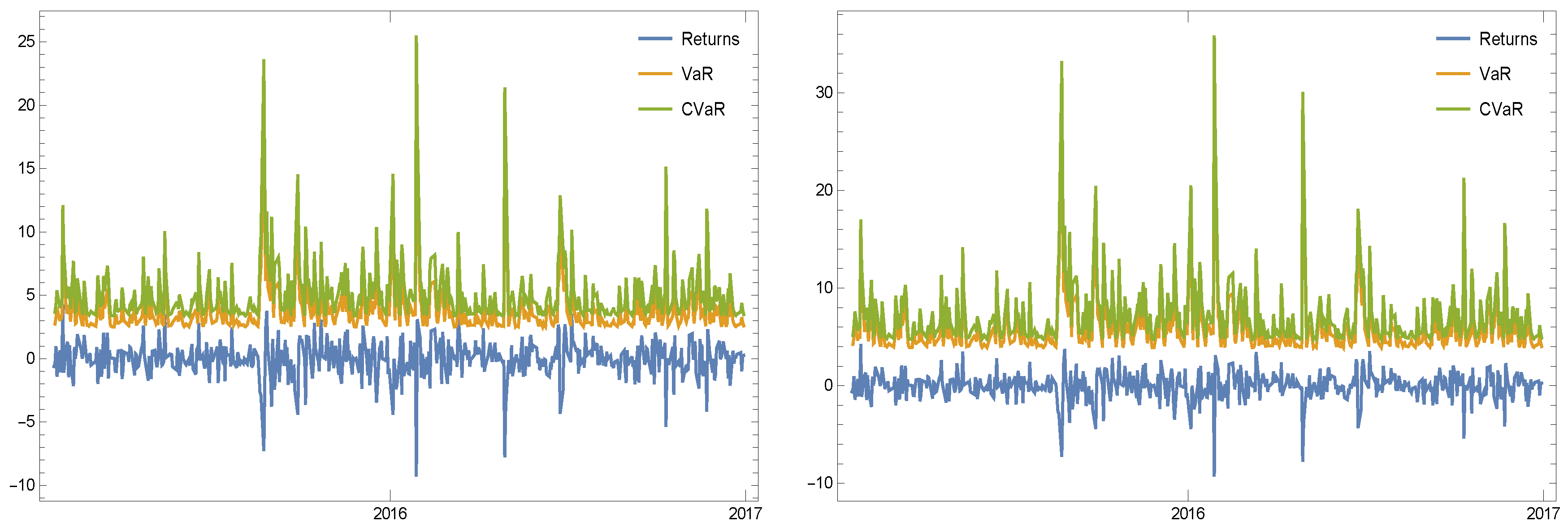
4. Discussion of Findings: Results and Simulations

The target of this section is to compare VaR and CVaR predictions employing the process of GARCH on controlling the risk happening for the trading days of an open stock in market mainly from S&P500. The data chosen here so as to be represented for a variety of different tickers of different sectors of the market. In the evaluation of VaR and CVaR, we consider the procedure based on 1-day ahead volatility forecast.
Note that the computational workouts in this work were done using the programming package Mathematica 12.0 [29] and Windows 10, Core i7-9750H CPU with 16GB of RAM on SSD memory.
It is well known that the VaR and CVaR under the normal distributions are given by
VaR ( normal ) = μ 2 σ erfc 1 ( 2 α ) ,
CVaR ( normal ) = μ σ e erfc 1 ( 2 α ) 2 2 π ( α 1 ) ,
where
erfc ( z ) = 1 2 π 0 z e t 2 d t ,
and implicity states that upon the choice of the same parameters and the tail level, we obtain
VaR ( EVT ) VaR ( normal ) , CVaR ( EVT ) CVaR ( normal ) .
This is compared further in Table 1. The empirical results from Table 2 show that larger scalarized values for the risk can be forecasted based on the application of VaR and CVaR under the EVD which also have higher value in contrast to the well-used normal distribution. This helps the investors to have more confidence of trading if the sudden stock’s price movement occur which may occur in severe gain or loss for the investor/trader. The results also revealing that the increased risk budget is adequate (i.e., we do not overestimate risk, by skyrocketing the risk budget and becoming overcautious).

4.1. Stocks

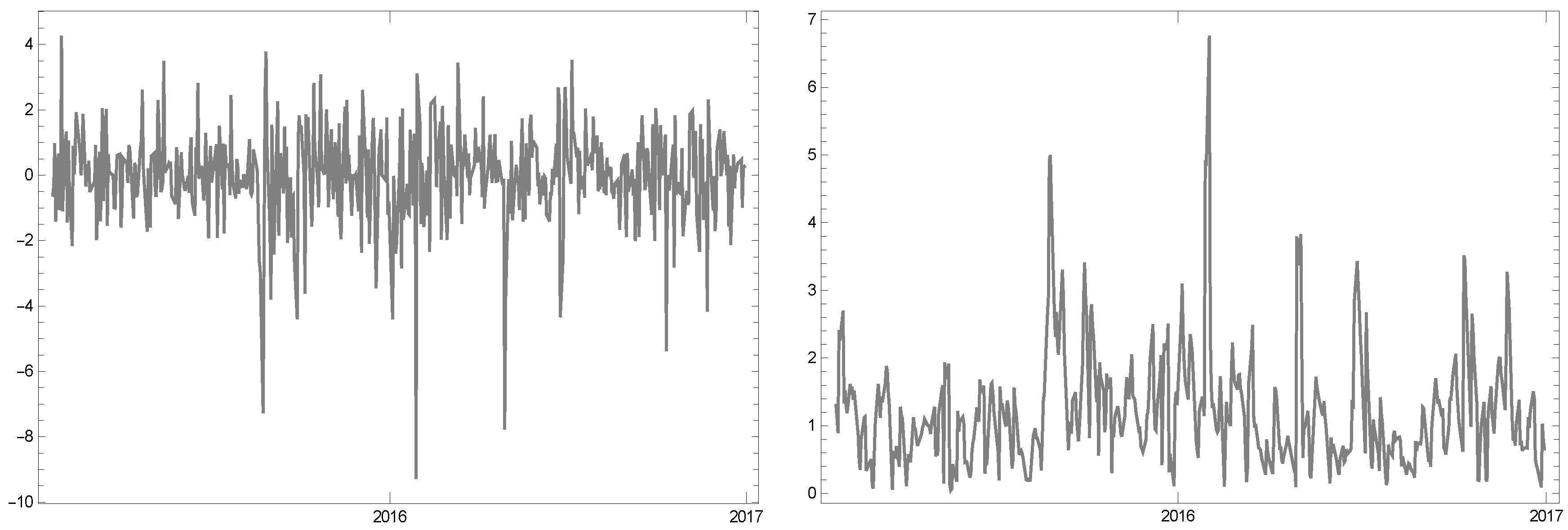
  • The first experiment is based on the stock’s ticker “NYSE:ABT” which is used during a specified period of time for checking the usefulness of the discussed risk measures. The information of this considered stock is furnished clearly in Table 2 and in Figure 2 based upon its newest (as of writing this work) trading volume and its available dates.
  • The second experiment is based on “NASDAQ:ZION”.
  • The third experiment is based on “NYSE:WMB”.
  • The fourth experiment is based on “NYSE:PG”. Basically, this is a test which has been conducted during the periods of different stock market dynamics (e.g., the financial crisis of 2008–2009), while the number of 755 observations are sufficient to judge of VaR/CVaR at 99%. Here, we have at least 1250 daily observations.
  • The fifth experiment is based on “NASDAQ:INTU”.

4.2. Empirical Results

Applying the model (7) on the returns of the stock (given in Figure 3) through a time series fitting approach [24] leads to the features in Table 3 and the covariance and information matrices [30], respectively, as follows:
A = 8.10926 9.11427 9.11427 11.0278 , B = 1.7347 1.4337 1.4337 1.27561 .
The computational results of the simulations given in Figure 4 for the first test, too, show that:
  • First of all, by increasing the pre-determined tail level, both measures tend to each other.
  • Choosing the pre-determined confidence level 95 % sounds to be a good choice for a highly volatile stock as long as we use such risk measures under the EVD.
It is recalled that several of the past approaches have considered normality or log-normality assumptions [31], that can occasionally provide misleading results since most financial and economic returns are featured by leptokurtosis (fat-tails) and skewness (asymmetry). Here, although the EVD has thin tail on the right side of its PDF, its fatter tail on the other side along with higher pre-determined tail level could yield good risk values/scalars in market.
For the other experiments coming from different sectors of the market and to save some space, the process of fitting the GARCH(1,1) [32], finding the parameters and computing the VaR and CVaR under the EVD is similar; thus, we now only plot the final results for different values of the predetermined confidence level α in Figure 5, Figure 6, Figure 7 and Figure 8. Results uphold the theoretical discussions given in Section 3 and Section 4 by illustrating that CVaR under the EVD is a good risk measures for the management of risk in market on various time frames. To summarize, the results revealed that the GARCH(1,1) process can successfully be employed along with the discussed VaR and CVaR risk measures to forecast the risk involved in the life time of a stock during a period of time.
Although the target of this work is on the general GARCH process for simulating the controlling the risk involved in trading, some may suggest to perform ARCH test and asymmetry test for S&P500 first, so as to avoid directly using GARCH model to compare the predicted performance of VaR and CVaR. This is originated mainly because, after verification, stock price information may be more suitable for estimation using the asymmetric GARCH model (for example exponential generalized autoregressive conditional heteroskedastic (E-GARCH) or the Glosten-Jagannathan-Runkle GARCH (GJR-GARCH)) and for comparing the forecast performance of VaR and CVaR. Recalling that the E-GARCH model by Nelson in Reference [33] is another form of the GARCH model and the GJR-GARCH model proposed in Reference [34] also models asymmetry in the ARCH process. In fact, for all of the GARCH-type models, the volatility process is different [19]. In order not to move away from our main focus, here we briefly compare the results of applying the well-known AR, ARCH, and GARCH process on the return of the last stock considered Section 4.1, i.e., NASDAQ:INTU. The results are provided in Table 4.
We also now use the property of Akaike information criterion (AIC) that measure goodness of fit by including several candidate selection table. Table 5 furnishes the results re-confirming based on AIC that GARCH(1,1) is a good choice, though some other models can also be employed.
Note that, for evaluating the accuracy of forecasting VaR for the proposed model, we should back-test the models using the Christoffersen likelihood ratio (CLR) test (see Reference [35]) and the Berkowitz test (see Reference [36]). This is a better way of evaluating the back-testing performance of the competitive models [37]. However, we will focus on this in future studies.
Since we basically analyzed the historical data, one question may still remain: How does the historical model affect the future? To respond this, when we first get the returns (or prices) and correspondingly obtain their associated risk measures under a risk metric, then one can obtain a time series model fit for the current behavior of the stock (pr its corresponding risk components); then, to forecast the future, we may do this by employing a time series forecast on the obtained results for a short piece of working days. This procedure yields a time series process (such as ARIMA(0,1,0)), which is employed for forecasting.

5. Conclusions

The application of CVaR in contrast to VaR tends to lead to a more practical way in terms of risk exposure. The selection between CVaR and VaR is not that clear from time to time for practitioners, but engineered and volatile investments can take advantage from CVaR as a double check to the assumptions considered by VaR.
In this paper, we have derived closed formulations and examined both risk metrics of VaR and CVaR for computing the risk under the EVD and demonstrated their application in the time series process. In fact, we proved how to compute the VaR and CVaR under the EVD which has right fat tail as an upper-hand over the well-used normal distribution. Understanding the volatility clustering and heteroskedasticity nature of time series, we have employed the GARCH(1,1) for modeling the time series coming from the returns of the stocks during a period of time. The GARCH process helped us in Section 4 to find some boundaries/values as scalarized risk over a given period of time for managing the risk. This could help the investors to forecast the risk involved in trading different tickers in the marker with a better (larger) consideration of risk over the time.
To contribute further on behavior of prices coming from market observations, an idea is to rely on a mixture distribution arising from the EVD ( μ , σ ) , at which σ is simulated based on a Rayleigh distribution with parameter λ . Such an investigation is under study in our research team and can be focused on as forthcoming works in this field.

Author Contributions

All authors contributed equally. All authors have read and agreed to the published version of the manuscript.

Funding

This project was supported by Researchers Supporting Project number (RSP-2020/210), King Saud University, Riyadh, Saudi Arabia.

Acknowledgments

We are thankful to three anonymous referees for several suggestions and comments.

Conflicts of Interest

The authors state that they have no known personal relationships or competing financial interests that could have appeared to affect the work reported in this work.

References

  1. Albrecher, H.; Binder, A.; Lautscham, V.; Mayer, P. Introduction to Quantitative Methods for Financial Markets; Springer: Basel, Switzerland, 2013. [Google Scholar]
  2. Bormetti, G.; Cisana, E.; Montagna, G.; Nicrosini, O. A non-Gaussian approach to risk measures. Phys. A 2007, 376, 532–542. [Google Scholar] [CrossRef] [Green Version]
  3. Galindo, J.; Tamayo, P. Credit risk assessment using statistical and machine learning basic methodology and risk modeling applications. Comput. Econ. 2000, 15, 107–143. [Google Scholar] [CrossRef]
  4. Markowitz, H. Portfolio selection. J. Financ. 1952, 7, 77–91. [Google Scholar]
  5. Roy, A. Safety first and the holding of assets. Econometrica 1952, 20, 431–449. [Google Scholar] [CrossRef]
  6. Lechner, L.A.; Ovaert, T.C. Value-at-risk: Techniques to account for leptokurtosis and asymmetric behavior in returns distributions. J. Risk Fin. 2010, 11, 464–480. [Google Scholar] [CrossRef]
  7. Altun, E.; Tatlidil, H.; Ozel, G.; Nadaraja, S. Does the Assumption on Innovation Process Play an Important Role for Filtered Historical Simulation Model? J. Risk Financ. Manag. 2018, 11, 7. [Google Scholar] [CrossRef] [Green Version]
  8. Benninga, S.; Wiener, Z. Value-at-Risk (VaR). Math. Edu. Res. 1998, 7, 1–8. [Google Scholar]
  9. Braione, M.; Scholtes, N.K. Forecasting value-at-risk under different distributional assumptions. Econometrics 2016, 4, 3. [Google Scholar] [CrossRef] [Green Version]
  10. Wang, Z.-R.; Chen, X.-H.; Jin, Y.-B.; Zhou, Y.-J. Estimating risk of foreign exchange portfolio: Using VaR and CVaR based on GARCH-EVT-Copula model. Phys. A 2010, 389, 4918–4928. [Google Scholar] [CrossRef]
  11. Soleymani, F.; Itkin, A. Pricing foreign exchange options under stochastic volatility and interest rates using an RBF-FD method. J. Comput. Sci. 2019, 37, 101028. [Google Scholar] [CrossRef] [Green Version]
  12. Sarykalin, S.; Serraino, G.; Uryasev, S. Value-at-risk vs. conditional value-at-risk in risk management and optimization. Informs 2008, 270–294. [Google Scholar] [CrossRef] [Green Version]
  13. Schmid, K.; Belzner, L.; Kiermeier, M.; Neitz, A.; Phan, T.; Gabor, T.; Linnhoff, C. Risk-sensitivity in simulation based online planning. In Proceedings of the 41st German Conference on AI, Berlin, Germany, 24–28 September 2018. [Google Scholar]
  14. Basel Committee on Banking Supervision. Minimum Capital Requirements for Market Risk; Basel Committee on Banking Supervision: Basel, Switzerland, January 2019. [Google Scholar]
  15. Williams, B. GARCH(1,1) Models; Ruprecht-Karls-Universität: Heidelberg, Germany, 2011. [Google Scholar]
  16. Halkos, G.E.; Tsirivis, A.S. Value-at-risk methodologies for effective energy portfolio risk management. Econ. Anal. Policy 2019, 62, 197–212. [Google Scholar] [CrossRef]
  17. Bollerslev, T. Generalized autoregressive conditional heteroskedasticity. J. Econom. 1986, 31, 307–327. [Google Scholar] [CrossRef] [Green Version]
  18. Hlivka, I. VaR, CVaR and Their Time Series Applications; Research Note; Quant Solutions Group: London, UK, 2015; pp. 1–2. [Google Scholar]
  19. Chu, J.; Chan, S.; Nadarajah, S.; Osterrieder, J. GARCH Modelling of Cryptocurrencies. J. Risk Financ. Manag. 2017, 10, 17. [Google Scholar] [CrossRef]
  20. Echaust, K.; Just, M. Value at risk estimation using the GARCH-EVT approach with optimal tail selection. Mathematics 2020, 8, 114. [Google Scholar] [CrossRef] [Green Version]
  21. Davis, R.A.; Mikosch, T. Extreme value theory for garch processes. In Handbook of Financial Time Series; Springer: Berlin/Heidelberg, Germany, 2009; pp. 187–200. [Google Scholar]
  22. Gilli, M.; Kellezi, E. An application of extreme value theory for measuring financial risk. Comput. Econ. 2006, 27, 1–23. [Google Scholar] [CrossRef] [Green Version]
  23. Norton, M.; Khokhlov, V.; Uryasev, S. Calculating CVaR and bPOE for common probability distributions with application to portfolio optimization and density estimation. Ann. Oper. Res. 2019. [Google Scholar] [CrossRef] [Green Version]
  24. McNeil, Q.J.; Frey, R.; Embrechts, P. Quantitative Risk Management, Revised ed.; Princeton University Press: Princeton, NJ, USA, 2015. [Google Scholar]
  25. Goode, J.; Kim, Y.S.; Fabozzi, F.J. Full versus quasi MLE for ARMA-GARCH models with infinitely divisible innovations. Appl. Econ. 2015, 47, 5147–5158. [Google Scholar] [CrossRef]
  26. Owusu-Ansah, E.D.J.; Barnes, B.; Donkoh, E.K.; Appau, J.; Effah, B.; Mccall, M. Quantifying economic risk: An application of extreme value theory for measuring fire outbreaks financial loss. Finan. Math. Appl. 2019, 4, 1–12. [Google Scholar]
  27. Tabasi, H.; Yousefi, V.; Tamošaitienė, J.; Ghasemi, F. Estimating conditional value at risk in the Tehran stock exchange based on the extreme value theory using GARCH models. Adm. Sci. 2019, 9, 40. [Google Scholar] [CrossRef] [Green Version]
  28. He, X.; Gong, P. Measuring the coupled risks: A copula-based CVaR model. J. Comput. Appl. Math. 2009, 223, 1066–1080. [Google Scholar] [CrossRef] [Green Version]
  29. Georgakopoulos, N.L. Illustrating Finance Policy with Mathematica; Springer International Publishing: Cham, Switzerland, 2018. [Google Scholar]
  30. Engle, R.F. Autoregressive conditional heteroskedasticity with estimates of the variance of U.K. inflation. Econometrica 1982, 50, 987–1008. [Google Scholar] [CrossRef]
  31. Aliyev, F.; Ajayi, R.; Gasim, N. Modelling asymmetric market volatility with univariate GARCH models: Evidence from Nasdaq-100. J. Econ. Asymmetries 2020, 22, e00167. [Google Scholar] [CrossRef]
  32. Herwartz, H. Stock return prediction under GARCH–An empirical assessment. Int. J. Forecast. 2017, 33, 569–580. [Google Scholar] [CrossRef]
  33. Nelson, D.B. Conditional heteroskedasticity in asset returns: A new approach. Econometrica 1991, 59, 347–370. [Google Scholar] [CrossRef]
  34. Glosten, L.R.; Jagannathan, R.; Runkle, D.E. On the relation between the expected value and the volatility of the nominal excess return on stocks. J. Financ. 1993, 48, 1779–1801. [Google Scholar] [CrossRef]
  35. Christoffersen, P.F. Evaluating interval forecasts. Int. Econ. Rev. 1998, 39, 841–862. [Google Scholar] [CrossRef]
  36. Berkowitz, J. Testing density forecasts, with applications to risk management. J. Bus. Econ. Stat. 2001, 19, 465–474. [Google Scholar] [CrossRef]
  37. Acerbi, C.; Szekely, B. Back-testing expected shortfall. Risk 2014, 27, 76–81. [Google Scholar]
Figure 1. Value-at-Risk (VaR) and Conditional VaR (CVaR) under the extreme value distribution (EVD) in left. The probability density functions (PDFs) of the two continuous distributions in right for μ = 0.01 and σ = 0.005 . Color figure can be viewed on the online version.
Symmetry 12 01698 g001
Figure 2. The trading volume of the Abbott Laboratories financial entity (left) and its data for all the available dates (right) by the time completing this work.
Symmetry 12 01698 g002
Figure 3. The return of the Abbott Laboratories stock (left) and its return volatility (right) on the considered time period.
Symmetry 12 01698 g003
Figure 4. The comparisons of the risk measures by the pre-determined tail level α = 95 % in left and α = 99 % in right for the NYSE:ABT. Color figure can be viewed on the online version.
Symmetry 12 01698 g004
Figure 5. The comparisons of the risk measures by the pre-determined tail level α = 95 % in left and α = 99 % in right for the NASDAQ:ZION. Color figure can be viewed on the online version.
Symmetry 12 01698 g005
Figure 6. The comparisons of the risk measures by the pre-determined tail level α = 95 % in left and α = 99 % in right for the NYSE:WMB. Color figure can be viewed on the online version.
Symmetry 12 01698 g006
Figure 7. The comparisons of the risk measures by the pre-determined tail level α = 95 % in left and α = 99 % in right for the NYSE:PG. Color figure can be viewed on the online version.
Symmetry 12 01698 g007
Figure 8. The comparisons of the risk measures by the pre-determined tail level α = 95 % in left and α = 99 % in right for the NASDAQ:INTU. Color figure can be viewed on the online version.
Symmetry 12 01698 g008
Table 1. Comparison of VaR and CVaR under normal and extreme value distributions.
μ σ α VaR(Normal)VaR(EVD)CVaR(Normal)CVaR(EVD)
0.020.0020.90.0220.0240.0230.026
0.020.0020.940.0230.0250.0230.027
0.020.0020.980.0240.0270.0240.029
0.020.0030.90.0230.0260.0250.029
0.020.0030.940.0240.0280.0250.031
0.020.0030.980.0260.0310.0270.034
0.020.0040.90.0250.0290.0270.033
0.020.0040.940.0260.0310.0270.035
0.020.0040.980.0280.0350.0290.039
0.020.0050.90.0260.0310.0280.036
0.020.0050.940.0270.0330.0290.038
0.020.0050.980.0300.0390.0320.044
0.030.0020.90.0320.0340.0330.036
0.030.0020.940.0330.0350.0330.037
0.030.0020.980.0340.0370.0340.039
0.030.0030.90.0330.0360.0350.039
0.030.0030.940.0340.0380.0350.041
0.030.0030.980.0360.0410.0370.044
0.030.0040.90.0350.0390.0370.043
0.030.0040.940.0360.0410.0370.045
0.030.0040.980.0380.0450.0390.049
0.030.0050.90.0360.0410.0380.046
0.030.0050.940.0370.0430.0390.048
0.030.0050.980.0400.0490.0420.054
0.040.0020.90.0420.0440.0430.046
0.040.0020.940.0430.0450.0430.047
0.040.0020.980.0440.0470.0440.049
0.040.0030.90.0430.0460.0450.049
0.040.0030.940.0440.0480.0450.051
0.040.0030.980.0460.0510.0470.054
0.040.0040.90.0450.0490.0470.053
0.040.0040.940.0460.0510.0470.055
0.040.0040.980.0480.0550.0490.059
0.040.0050.90.0460.0510.0480.056
0.040.0050.940.0470.0530.0490.058
0.040.0050.980.0500.0590.0520.064
Table 2. The features of the considered stocks.
NameTicker SymbolExchangeSectorFloat SharesStart TimeEnd TimeData Points
Abbott LaboratoriesNYSE:ABTNYSEMedical Devices176739761516 Jan. 201530 Dec. 2016492
Zions Bancorp NANASDAQ:ZIONNasdaqBanks Regional17696299616 Jan. 201530 Dec. 2016493
Williams Companies Inc.NYSE:WMBNYSEOil And Gas Midstream121202239801 Jan. 202026 June 2020121
Procter & GambleNYSE:PGNYSEHousehold And Personal Products250263312004 Jan. 200631 Dec. 20101258
Intuit IncNASDAQ:INTUNasdaqSoftware Application25924338501 Jan. 202026 June 2020121
Table 3. Fitted parameters of the generalized autoregressive conditional heteroskedasticity (GARCH)(1,1) model for the first experiment.
w λ β Error Variance
0.7225420.1859680.46482626.6742
Table 4. Fitted parameters of for various variance processes for the ticker NASDAQ:INTU.
w λ β
GARCH(1,1)0.6288760.1394260.813362
w λ 1 λ 2 λ 3 λ 4
ARCH(4)5.299240.08581450.1989130.1760510.14139
AR(0)w λ
0.10302613.3097
Table 5. The candidate selection results for the ticker NASDAQ:INTU.
#CandidateAIC
1GARCHProcess(1,1)1254.61
2GARCHProcess(0,1)1285.77
1ARCHProcess(4)1260.03
2ARCHProcess(3)1261.61
3ARCHProcess(5)1261.80
4ARCHProcess(2)1266.24
5ARCHProcess(1)1276.89
6ARCHProcess(0)1283.77
1ARProcess(0)459.57
2ARProcess(1)461.45
Publisher’s Note: MDPI stays neutral with regard to jurisdictional claims in published maps and institutional affiliations.

