An Analysis of the KDD99 and UNSW-NB15 Datasets for the Intrusion Detection System

Abstract

The significant increase in technology development over the internet makes network security a crucial issue. An intrusion detection system (IDS) shall be introduced to protect the networks from various attacks. Even with the increased amount of works in the IDS research, there is a lack of studies that analyze the available IDS datasets. Therefore, this study presents a comprehensive analysis of the relevance of the features in the KDD99 and UNSW-NB15 datasets. Three methods were employed: a rough-set theory (RST), a back-propagation neural network (BPNN), and a discrete variant of the cuttlefish algorithm (D-CFA). First, the dependency ratio between the features and the classes was calculated, using the RST. Second, each feature in the datasets became an input for the BPNN, to measure their ability for a classification task concerning each class. Third, a feature-selection process was carried out over multiple runs, to indicate the frequency of the selection of each feature. From the result, it indicated that some features in the KDD99 dataset could be used to achieve a classification accuracy above 84%. Moreover, a few features in both datasets were found to give a high contribution to increasing the classification’s performance. These features were present in a combination of features that resulted in high accuracy; the features were also frequently selected during the feature selection process. The findings of this study are anticipated to help the cybersecurity academics in creating a lightweight and accurate IDS model with a smaller number of features for the developing technologies.

1. Introduction

Due to the increasing demand for computer networks and network technologies, the attack incidents are growing day by day, making the intrusion detection system (IDS) an essential tool to use for keeping the networks secure. It has been proven to be effective against many different attacks, such as the denial of service (DoS), structured query language (SQL) injection, and brute-force [1,2,3]. Two approaches are to be considered when developing an IDS [4]: misuse-based and anomaly-based. In the misuse-based approach, the IDS attempts to match the patterns of already known network attacks. Its database gets updated continuously by storing the patterns of known network attacks. The anomaly-based IDS, on the other hand, attempts to detect unknown network attacks by comparing them to the regular connection patterns. The anomaly-based IDSs are considered to be adaptive, and they are susceptible to generate a high number of false positives [4,5].

For developing an efficient IDS model, a large amount of data is required for training and testing. The quality of the data is very critical and influential, primarily on the results of the IDS model [6]. The low-quality and irrelevant information found in data can be eliminated after gathering the statistical properties from its observable attributes and elements [7]. However, the data could be insufficient, incomplete, imbalanced, high-dimensional, or abundant [6]. Therefore, providing an in-depth analysis of the available datasets is crucial for IDS research.

The KDD99 [8] and UNSW-NB15 [9,10] datasets are two well-known available IDS datasets. Many studies have used these datasets in their works [11,12,13,14,15,16,17,18,19,20,21]. Reference [11] introduced a new hybrid method for classification based on two algorithms, namely artificial fish swarm (AFS) and artificial bee colony (ABC). The hybrid method was tested by using the UNSW-NB15 and NSL-KDD datasets. Reference [12] proposed a wrapper approach that uses different decision-tree classifiers and was tested by using the KDD99 and UNSW-NB15 datasets. Reference [13] presented a hybrid C4.5 and modified K-means and evaluated it, using the KDD99. References [14,15] used the KDD99 to evaluate a hybrid classification method based on an extreme learning machine (ELM) and support vector machine (SVM). Reference [16] introduced a hybrid classification method that utilized the K-means and information gain ratio (IGR) and evaluated the method, using the KDD99 dataset. Reference [17] introduced a methodology of combining datasets (called MapReduce). In their work, they used the KDD99 and DARPA datasets to test the introduced combination method. Then, they analyzed the combined and cleaned dataset, using K2 and NaïveBayes techniques. Reference [18] used the UNSW-NB15 dataset to evaluate an SVM with a new scaling approach. Reference [19] gave a comprehensive study on applying the local clustering approach to solve the IDS problem. For evaluation, the KDD99 dataset was utilized. Reference [20] employed a multi-layer SVM and tested it by using the KDD99 dataset. Different samples were selected from the dataset, which was used to evaluate the performance of their proposed method. Reference [21] proposed a novel discrete metaheuristic algorithm, a discrete cuttlefish algorithm (D-CFA), to solve the feature selection problem. The D-CFA was tested, to reduce the features in the KDD99 dataset. The algorithm was introduced based on the color reflection and visibility mechanism of the cuttlefish. Few more variants of the algorithm were proposed in the literature [22,23]. However, the selected features by the D-CFA in Reference [21] were evaluated by a decision tree (DT) classifier. The study found that the classifier achieved a 91% detection rate and a 3.9% false-positive rate with only five selected features.

Furthermore, only a few studies have tried to analyze the KDD99 and UNSW-NB15 datasets [7,24,25,26,27,28,29,30]. Reference [24] used a clustering method and an integrated rule-based IDS to analyze the UNSW-NB15 dataset. Reference [25] analyzed the relation between the attacks in the UNSW-NB15 and their transport layer protocols (transmission control protocol and user datagram protocol). Reference [26] gave a case study on the KDD99 dataset. The study stated a lack of works in the IDS research that analyzes the currently available datasets. In Reference [27], the characteristics of the features in the KDD99 and UNSW-NB15 datasets were investigated for effectiveness measurement. An association rule mining algorithm and a few other existing classifiers were used for their experiments. The study claimed that UNSW-NB15 offers more efficient features than the KDD99 in detection accuracy and the number of false alarms. Reference [28] analyzed the KDD99 and proposed a new dataset, called NSL-KDD, an improved version of the KDD99. Reference [7] also gave an analysis of the KDD99. Besides, they analyzed other variants, namely the NSL-KDD and GureKDDcup datasets. The analysis in Reference [7] was aimed to improve the datasets by reducing the dimensions, completing missing values, and removing any redundant instances. The study found that KDD99 contains a high number of redundant instances. Reference [29] used a rough-set theory (RST) to measure the relationship between the features and each class in the KDD99. In the study, a few features were classified as not relevant for any of the dataset’s classes. Reference [30] gave an analysis of the feature relevance of the KDD99, using an information gain. The study concluded that a few features in the dataset do not contribute to the attack detection. It also concluded that the testing set of the dataset offers different characteristics than its training set.

Recently, Reference [31] surveyed the available datasets in the IDS research and gave a comprehensive overview of the properties of each dataset. The first property discussed in the study was general information, such as the year and type of classes. The second property was the data nature, covering the formatting and information about metadata, if existing in the dataset. The third property was the size and duration of the captured packets. The fourth property included the recording environment, which indicated the type of traffic and network’s services used for the dataset generation. Lastly, the evaluation part provided for the researchers, for example, the class balance and the predefined data split. However, Reference [31] recommended the researchers to produce a dataset that is focused on specific attack types rather than trying to cover all the possible attacks. If the dataset satisfies a specific application, then it is considered sufficient. In Reference [31], the comprehensive dataset was described to have correctly labeled classes available for everyone, include real-world network traffic and not synthetic, contain all kinds of attacks, and be always updated. It should also contain packets header information and the data payload, which needs to be captured over a long period. Based on the number of attacks provided in the available datasets, the UNSW-NB15 was one of their general recommendations for IDS testing.

Reference [32] reviewed a few of the IDS datasets, namely full KDD99, corrected, and ten percent variants of the KDD99, NSL-KDD, UNSW-NB15, center for applied internet data analysis dataset (CAIDA), australian defence force academy linux dataset (ADFA-LD), and university of new mexico dataset (UNM). The study in Reference [32] gave general information for each of the datasets, with more emphasis on UNSW-NB15. For comparison, the k-nearest neighbors (k-NN) classifier was implemented to report the accuracy, precision, and recall across all the reviewed datasets. The results showed that the classifier performed better when using the NSL-KDD. They claimed that the superior results from using the NSL-KDD were achieved because the dataset contains less redundant records, which are distributed fairly. Reference [33] analyzed the KDD99, NSL-KDD, and UNSW-NB15 datasets, using a deep neural network (DNN) on the internet of things (IoT). By applying a similar evaluation metric as in Reference [32] and F1 measure, the results show that DNN was able to achieve an accuracy above 90% for all datasets. Further, DNN had the best performance on UNSW-NB15. Reference [34] evaluated the features in the NSL-KDD and UNSW-NB15, using four filter-based feature-selection measures, namely correlation measure (CFS), consistency measure (CBF), information gain (IG), and distance measure (ReliefF). The selected features from those four methods were then evaluated by using four classifiers to indicate the training and testing performance, namely k-NN, random forests (RF), support vector machine (SVM), and deep belief network (DBN). The study reported the selected features for each feature selection method, in addition to the classification results, which were aimed to provide help for the researchers in the cybersecurity in designing affective IDS. Reference [35] analyzed the UNSW-NB15 dataset by finding the relevance of the features, using a neural network. The authors categorized the features into five groups, based on their type, such as flow-based, content-based, time-based, essential, and additional features. From these groups, 31 possible combinations of features were evaluated and discussed. The highest accuracy (93%) in Reference [35] was obtained by using 39 features from the categorized groups. Moreover, in the study, there was a combination of 23 features that were selected by using a meta estimator called SelectFromModel that selects features based on their scores. The 23 selected features resulted in higher accuracy (97%) than those 39 features mentioned above.

Reference [36] compared the features in the UNSW-NB15 dataset with a few feature vectors that were previously proposed in the literature. They were evaluated by using a supervised machine learning to indicate the computational times and classification performance. The results of the study suggested that the current vectors can be improved by reducing their size and adapting them to deal with encrypted traffic. Reference [37] proposed a feature-selection method based on the genetic algorithm (GA), grey wolf optimizer (GWO), particle swarm optimization (PSO), and firefly optimization (FFA). The UNSW-NB15 dataset was employed for the tests of the study. The selected features from using the proposed method were evaluated by using SVM and J48 classifiers. The study reported the classification performance of a few combinations of features from the UNSW-NB15 dataset. In Reference [38], a hierarchical IDS that uses machine-learning and knowledge-based approaches was introduced and tested, using the KDD99 dataset. Reference [39] proposed an ensemble model based on the J48, RF, and Reptree and evaluated it by using the KDD99 and NSL-KDD datasets. A correlation-based approach was implemented, to reduce the features from the datasets. Reference [40] examined the reliability of a few machine learning models, such as the RF and gradient-boosting machines in real-world IoT settings. In order to do the examination, data-poisoning attacks were simulated by using a stochastic function to modify the training data of the datasets. The UNSW-NB15 and ToN_IoT datasets were employed for the experiments of the study.

It is essential to address that the KDD99 and UNSW-NB15 datasets do not contain attacks related to the cloud computing, such as the SQL injection. Reference [41] proposed a countermeasure to detect these attacks, specifically in the cloud environment. The method in Reference [41] can be applied to the cloud environment, without the need for an application’s source code.

In this study, the features in the KDD99 and UNSW-NB15 datasets were analyzed by using a rough-set theory (RST), a back-propagation neural network (BPNN), and a discrete variant of the cuttlefish algorithm (D-CFA). The analysis provides an in-depth examination of the relevance of each feature to the malicious-attack classes. It also studies the symmetry of the records distribution among the classes. The results of the analysis suggest a few features and combinations that can be used for creating an accurate IDS model. This study also describes and gives the properties of the datasets mentioned above. Despite the availability of other works that have tried to analyze the two datasets, it is important to study the most common datasets in this domain continuously, not only to confirm their relevance but also to expand the findings on these datasets. However, the main contributions of this paper can be listed as follows:

• Give a detailed description of the KDD99 and UNSW-NB15 datasets.
• Point out the similarities between the two datasets.
• Indicate if the KDD99 is still relevant for the IDS domain.
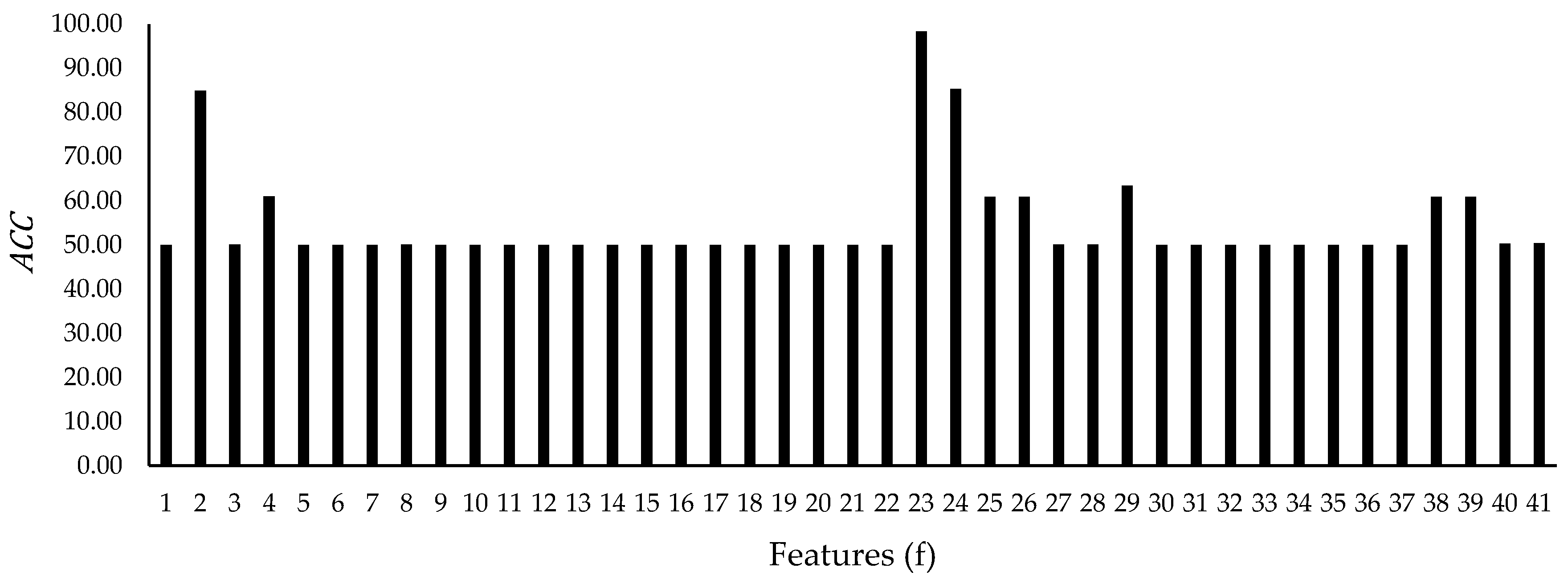
• List the relevant features for increasing the classification performance.
• Provide the statistical and properties of each feature concerning the classes.
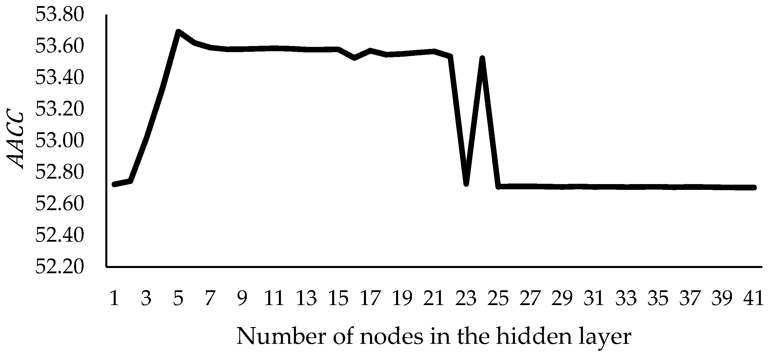
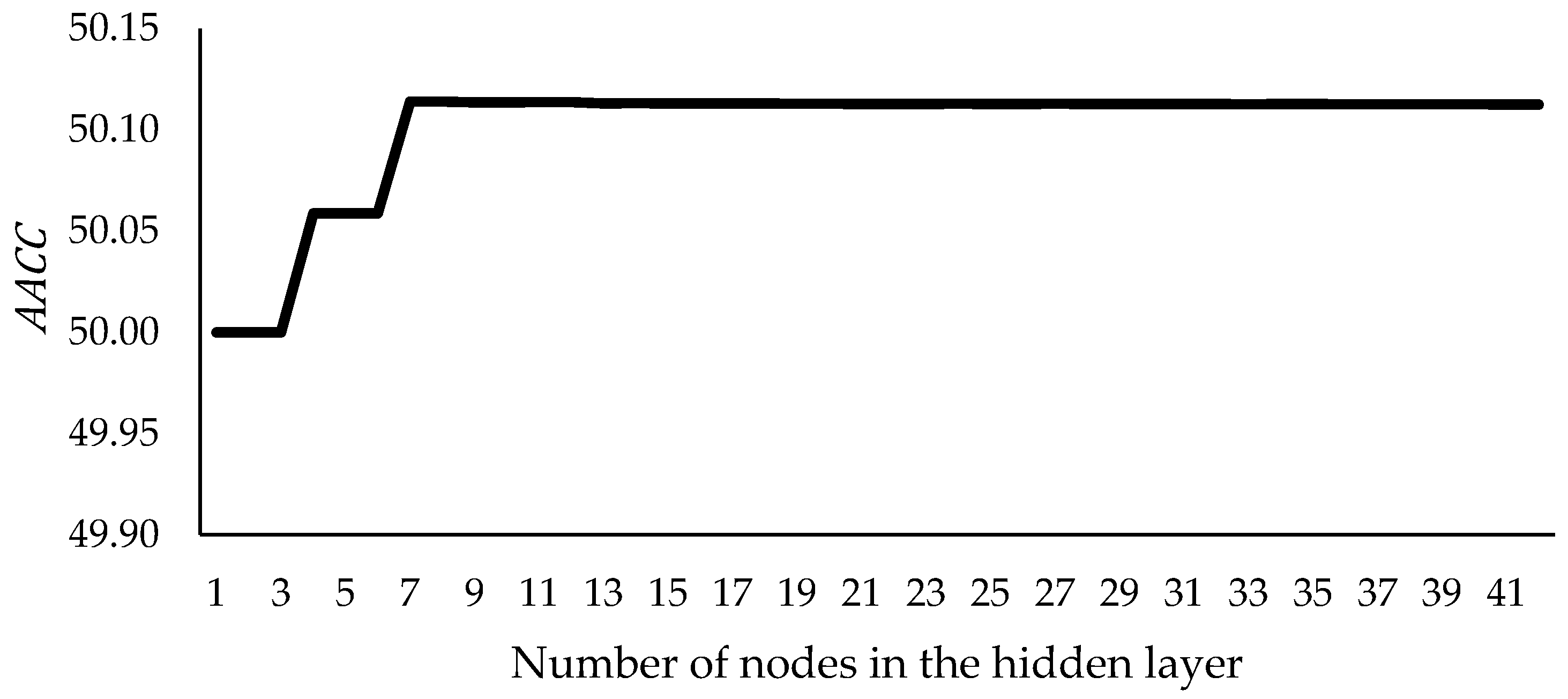
• Indicate the effect of the features in both datasets on the behavior of the neural networks.

This paper includes five sections. The description and properties of the KDD99 and UNSW-NB15 datasets are provided in Section 2. Section 3 explains the methodology and experimental setup. The results and discussions are given in Section 4. Conclusion and future work are provided in Section 5.

2. Datasets’ Description and Properties

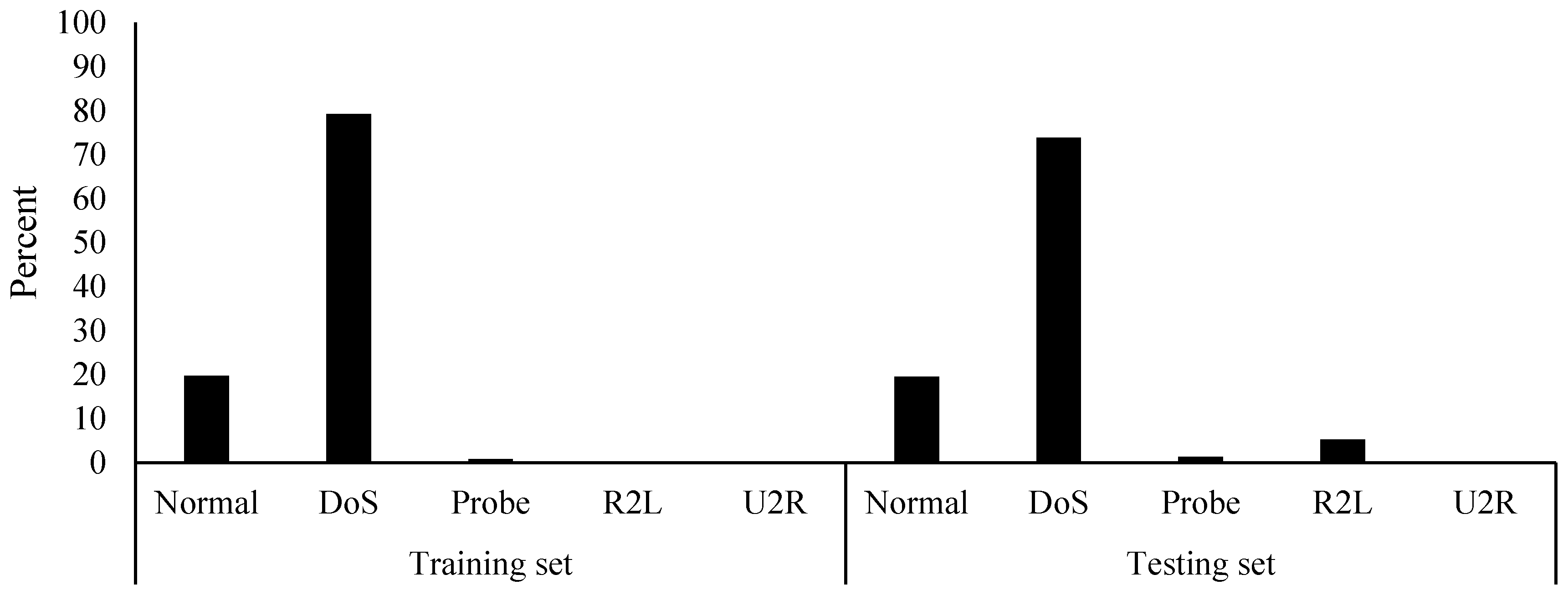
The KDD99 is very common between researchers in the IDS research. A survey by Reference [42] found that 142 studies have used the KDD99 dataset form year 2010 until 2015. The dataset is available with 41 features (excluding the labels) and five classes, namely Normal, DoS), Probe, remote-to-local (R2L), and user-to-root (U2R). The KDD99 (ten percent variant) contains 494,021 and 311,029 records in the training and testing sets. The classes in the training and testing sets of the KDD99 are imbalanced, as shown in Figure 1. The DoS class has the highest number of records, while the Normal class comes in second. Moreover, the testing set contains a higher amount of records that are classified as R2L. This distribution of records was found to contain a large amount of duplicated records. The number of records of each class with their amount of duplications is provided in

Table 1. The amount of duplications in the training and testing sets of the KDD99.

Class	Training Set			Testing Set
	No. of Duplicates	No. of Records	Duplicates Percentage	No. of Duplicates	No. of Records	Duplicates Percentage
All	348,437	494,021	70.53	233,813	311,029	75.17
Normal	9446	97,278	09.71	12,680	60,593	20.92
DoS	336,886	391,459	86.05	206,285	229,853	89.74
Probe	1977	4107	48.13	1488	4166	35.71
R2L	127	1126	11.27	13,276	16,189	82.00
U2R	0	52	0.00	13	228	5.70

.

A graphical representation of the amount of records duplications for each class is given in Figure 2. The highest amount of duplications in the training set belongs to DoS and Probe classes, whereas the highest amount of duplications in the testing set belongs to DoS and R2L. The Probe class in the testing set also contains a fair amount of duplications. It is essential to address that the U2R class contains no duplications in the training set. However, the full training and testing sets of the KDD99 dataset contain duplicated records of 348,437 (70.53%) and 233,813 (75.17%), respectively. Five percent more duplications were present in the testing set.

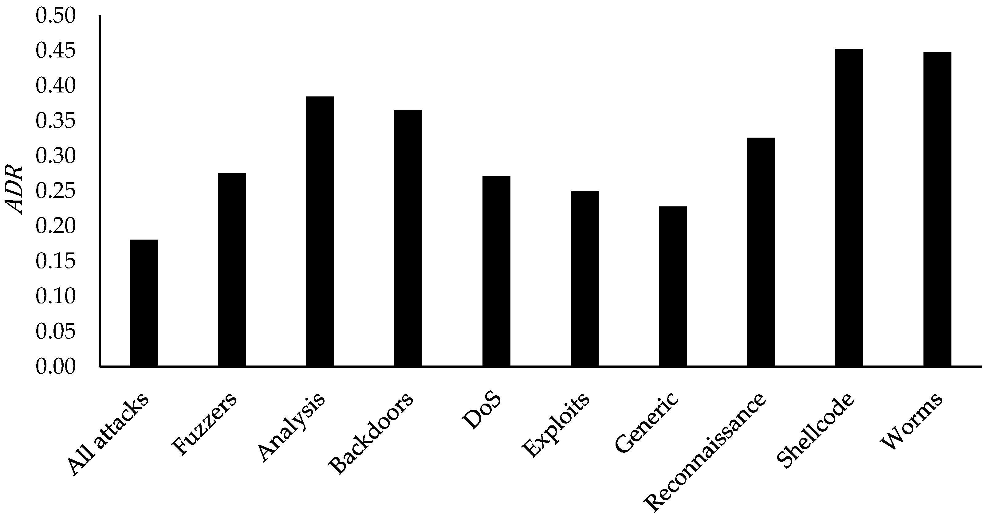
The available UNSW-NB15 dataset contains 42 features (excluding the labels) and ten classes, namely Normal, Fuzzers, Analysis, Backdoors, DoS, Exploits, Generic, Reconnaissance, Shellcode, and Worms. Its training set includes 175,341 records, while the testing set has 82,332 records. The classes in the training and testing sets of the UNSW-NB15 are also imbalanced, as illustrated in Figure 3. Normal class in both sets contains the highest amount of records. In contrast, Generic and Exploits come in second. Fuzzers class includes a fair amount of records, as well, but the rest of the classes show a low amount of records compared to the mentioned classes. However, it was found that the training set of the UNSW-NB15 contains a high number of duplicated records, whereas the testing set does not contain any. Based on the details given in

Table 2. The amount of duplications in the training and testing sets of the UNSW-NB15 dataset.

Class	Training Set			Testing Set
	No. of Duplicates	No. of Records	Duplicates Percentage	No. of Duplicates	No. of Records	Duplicates Percentage
All	74,072	175,341	42.24	0	82,332	0.00
Normal	4110	56,000	7.33	0	37,000	0.00
Fuzzers	2034	18,184	11.18	0	6062	0.00
Analysis	405	2000	20.25	0	677	0.00
Backdoors	211	1746	12.08	0	583	0.00
DoS	8457	12,264	68.95	0	4089	0.00
Exploits	13,548	33,393	40.57	0	11,132	0.00
Generic	35,819	40,000	89.54	0	18,871	0.00
Reconnaissance	2969	10,491	28.30	0	3496	0.00
Shellcode	42	1133	3.70	0	378	0.00
Worms	3	130	2.30	0	44	0.00

, the full training set shows that it contains 42.24% duplicated records. Figure 4 illustrates the duplications for each class in the training set. These duplications are found mainly in the Generic, DoS, and Exploits classes. Reconnaissance class also contains a fair amount of duplications.

The class distribution difference between the two datasets is shown in Figure 5. The KDD99 has a higher amount of records that represent a malicious attack class. Both training and testing sets of the KDD99 have an almost identical percentage of attack and normal records. As for the UNSW-NB15, the records distributions between the attack and normal classes are more balanced than those in the KDD99. Moreover, the percentage of the attacks and normal classes across both sets are slightly different.

The names of the features in each dataset are given in

Table 3. KDD99 and UNSW-NB15 list of features.

KDD99		UNSW-NB15
Feature	Name	Feature	Name
f1-1	duration	f2-1	Dur
f1-2	protocol_type	f2-2	Proto
f1-3	service	f2-3	Service
f1-4	flag	f2-4	State
f1-5	src_bytes	f2-5	Spkts
f1-6	dst_bytes	f2-6	Dpkts
f1-7	land	f2-7	Sbytes
f1-8	wrong_fragment	f2-8	Dbytes
f1-9	urgent	f2-9	Rate
f1-10	hot	f2-10	Sttl
f1-11	num_failed_logins	f2-11	Dttl
f1-12	logged_in	f2-12	Sload
f1-13	lnum_compromised	f2-13	Dload
f1-14	lroot_shell	f2-14	Sloss
f1-15	lsu_attempted	f2-15	Dloss
f1-16	lnum_root	f2-16	Sinpkt
f1-17	lnum_file_creations	f2-17	Dinpkt
f1-18	lnum_shells	f2-18	Sjit
f1-19	lnum_access_files	f2-19	Djit
f1-20	lnum_outbound_cmds	f2-20	Swin
f1-21	is_host_login	f2-21	Stcpb
f1-22	is_guest_login	f2-22	Dtcpb
f1-23	count	f2-23	Dwin
f1-24	srv_count	f2-24	Tcprtt
f1-25	serror_rate	f2-25	Synack
f1-26	srv_serror_rate	f2-26	Ackdat
f1-27	rerror_rate	f2-27	Smean
f1-28	srv_rerror_rate	f2-28	Dmean
f1-29	same_srv_rate	f2-29	trans_depth
f1-30	diff_srv_rate	f2-30	response_body_len
f1-31	srv_diff_host_rate	f2-31	ct_srv_src
f1-32	dst_host_count	f2-32	ct_state_ttl
f1-33	dst_host_srv_count	f2-33	ct_dst_ltm
f1-34	dst_host_same_srv_rate	f2-34	ct_src_dport_ltm
f1-35	dst_host_diff_srv_rate	f2-35	ct_dst_sport_ltm
f1-36	dst_host_same_src_port_rate	f2-36	ct_dst_src_ltm
f1-37	dst_host_srv_diff_host_rate	f2-37	is_ftp_login
f1-38	dst_host_serror_rate	f2-38	ct_ftp_cmd
f1-39	dst_host_srv_serror_rate	f2-39	ct_flw_http_mthd
f1-40	dst_host_rerror_rate	f2-40	ct_src_ltm
f1-41	dst_host_srv_rerror_rate	f2-41	ct_srv_dst
		f2-42	is_sm_ips_ports

. The features in the KDD99 dataset are categorized into four groups. They are given in

Table 4. The four groups of features in the KDD99 dataset.

Group	Features	Count
Basic	f1-1, f1-2, f1-3, f1-4, f1-5, f1-6, f1-7, f1-8, f1-9	9
Content	f1-10, f1-11, f1-12, f1-13, f1-14, f1-15, f1-16, f1-17, f1-18, f1-19, f1-20, f1-21	13
Time	f1-23, f1-24, f1-25, f1-26, f1-27, f1-28, f1-29, f1-30, f1-31	9
Host	f1-32, f1-33, f1-34, f1-35, f1-36, f1-37, f1-38, f1-39, f1-40, f1-41	10

. The first group (basic) contains nine features that include necessary information, such as the protocol, service, and duration. The second group (content) represents thirteen features, containing information about the content, such as the login activities. The third group (time) provides nine time-based features, such as the number of connections that are related to the same host within two seconds period. The fourth (host) contains ten host-based features, which provide information about the connection to the host, such as the rate of connections that have the same destination port number trying to be accessed by different hosts.

As for the features in the UNSW-NB15 dataset, they are categorized into five groups and provided in

Table 5. The five groups of features in the UNSW-NB15 dataset.

Group	Features	Count
Flow	f2-2	1
Basic	f2-1, f2-3, f2-4, f2-5, f2-6, f2-7, f2-8, f2-9, f2-10, f2-11, f2-12, f2-13, f2-14, f2-15	14
Content	f2-20, f2-21, f2-22, f2-23, f2-27, f2-28, f2-29, f2-30	8
Time	f2-16, f2-17, f2-18, f2-19, f2-24, f2-25, f2-26, f2-42	8
Additional	f2-31, f2-32, f2-33, f2-34, f2-35, f2-36, f2-37, f2-38, f2-39, f2-40, f2-41	11

. The first group (flow) includes the protocol feature, which identifies the protocols between the hosts, such as a TCP or UDP. The second group (basic) represents the necessary connection information, such as the duration and number of packets between the hosts. Fourteen features are categorized in this group. The third group (content) provides content information from the TCP, such as the window advertisement values and base sequence numbers. It also provides some information about the HTTP connections, such as the data size transferred using the HTTP service. Eight features are present in this group. The fourth group (time) includes eight features that use time, such as the jitter and arrival time of the packets. The fifth group (additional) includes eleven additional features, such as if a login was successfully made. Moreover, the fifth group includes a few features that calculate the number of rows that use a specific service from a flow of 100 records based on a sequential order. It is important to address that a few described features in Reference [9], namely srcip, sport, dstip, dsport, stime, and ltime, were not present in the actual dataset; therefore, they were not included in this study. Moreover, f_2-9 was present in the dataset but was not described or categorized in Reference [9]; therefore, it was categorized in the basic group.

A few features were found to be in common between the two datasets. KDD99′s features f_1-1, f_1-2, f_1-3, f_1-5, and f_1-6 are in common with UNSW-NB15′s features f_2-1, f_2-2, f_2-3, f_2-7, and f_2-8. f_1-1 and f_2-1 describe the connection duration; f_1-2 and f_2-2 give the protocol type, such as transmission control protocol (TCP) or user datagram protocol (UDP); f_1-3 and f_2-3 state the service used at the destination, such as file transfer protocol (FTP) or domain name system (DNS); and f_1-5, f_2-7, f_1-6, and f_2-8 give the number of transmitted data bytes between the source and destination. There are some other features in between the two datasets that share similar characteristics. As described in

Table 6. Similarities of the features in KDD99 and UNSW-NB15.

Category	KDD99	UNSW-NB15
Common features	f1-1, f1-2, f1-3, f1-5, f1-6	f2-1, f2-2, f2-3, f2-7, f2-8
Features that use connection flags	f1-4, f1-9, f1-24, f1-25, f1-29, f1-30, f1-38, f1-39, f1-40, f1-41	f2-4, f2-24, f2-25, f2-26
Features that count connections	f1-5, f1-6, f1-23, f1-24, f1-25, f1-26, f1-27, f1-28, f1-29, f1-30, f1-31, f1-32, f1-33, f1-34, f1-35, f1-36, f1-37, f1-38, f1-39, f1-40, f1-41	f2-31, f2-33, f2-34, f2-35, f2-36, f2-40, f2-41
Size-based features (transmitted bits, bytes, or packets)	f1-5, f1-6	f2-5, f2-6, f2-7, f2-8, f2-12, f2-13, f2-14, f2-15, f2-27, f2-28, f2-30
Features that calculates time (e.g., connection duration)	f1-1, f1-23, f1-28	f2-1, f2-10, f2-11, f2-18, f2-19, f2-24, f2-25, f2-26

, both datasets contain features that use connection flags. Connection flags provide additional information, such as synchronization (SYN) and acknowledgment (ACK). There were ten features in the KDD99 that use flags, whereas, in the UNSW-NB15, there were only four features. In Table 6, it can also be seen that the number of features that involve connection count is higher in the KDD99 than UNSW-NB15. Further, the UNSW-NB15 was found to contain more features that are time-based and size-based.

3. Methodology

The dataset analysis was done by using three methods, namely RST, back-propagation neural network (BPNN), and D-CFA. First, using the RST, the dependency between the features and each of the attack classes was calculated. Second, using the BPNN, the classification accuracy ($ACC$) for each feature to detect a malicious attack class was computed. Lastly, the D-CFA was used for feature selection to select the most relevant features over multiple iterations and runs to indicate the most frequently selected features. The BPNN was recruited to evaluate those selected features as a wrapper feature selection approach. However, to calculate the $ACC$ from the BPNN, the records in the datasets were first transformed and normalized. Figure 6 illustrates the main steps that were taken to analyze the KDD99 and UNSW-NB15 datasets.

The three used methods for the analysis and their evaluation measurements are explained in detail in the following subsections.

3.1. Rough-Set Theory (RST)

The RST was used to find the dependency between the features and the classes. For this analysis, each feature was used to calculate its dependency on each of the malicious-attack classes. Based on References [29,43], the dependency ratio (called $depRatio$) was calculated, using Equation (1).

$$depRatio\left(X\right)=\left|\frac{lower\left(X\right)}{U}\right|$$

(1)

where $U$ denotes all the records, and $X$ signifies the cardinality of records that are used to classify two classes—normal and attack. The $depRatio$ is a value between 0 and 1. If the $depRatio$ = 1, then $X$ is a crisp set and can classify the two classes correctly, and if the $depRatio$ < 1, then $X$ is a rough set with a $depRatio$ value less than 1. It is defined based on the lower approximation (called $lower$), which is calculated by using Equation (2).

$$lower\left(X\right)=\{r|{\left[r\right]}_f\in X\}$$

(2)

where $lower\left(X\right)$ is the set of records that only belong to the target decision ($X$), which can be used to classify the decision without any uncertainty. It is the union of all the records for both classes in ${\left[r\right]}_f$, which are entirely contained by the selected feature ($f$). However, once the $depRatio\left(X\right)$ of the features is calculated, then, an average of that $depRatio$ (called $ADR$) can be computed, using Equation (3).

$$ADR=\frac{{{\displaystyle \sum }}_{i=1}^{n}depRatio\left(X\right)}{n}$$

(3)

where $n$ is the number of features in the dataset. The $ADR$ can be used to indicate the dependency of all the features to a specific attack class where a higher $ADR$ value designates a higher dependency.

3.2. Back-Propagation Neural Network (BPNN)

The used BPNN was based on its implementation provided in Reference [44]. The back-propagation is the training algorithm for adjusting the weights and biases of the neural network [44].

Formally, as illustrated in Figure 7, every input, $in{p}_i$, with weight, $w_i$, corresponds to the power of the connection. The sum of the weights and the bias, $b,$ donate to the activation function, $\sigma$, to generate the output, $y$ [45]. This process can be demonstrated by using Equation (4).

$$y=\sigma \left({\displaystyle \sum }_{i=1}^{n}in{p}_i{w}_i+b\right)$$

(4)

In order to keep the structure of the neural network simple, only one layer was set at the hidden layer. As for nodes in the hidden layer, a different number of nodes were set and evaluated with a maximum number equal to $n$. The logistic sigmoid function was used as an activation function at the hidden and output layers, using Equation (5).

$$\sigma \left(v_i\right)=\frac{1}{1+e^{-v_i}}$$

(5)

where $e$ is exponential, and $v_i$ represents the input value of the function.

Mean square error (MSE) was used to calculate the error loss during the training of the neural network, using Equation (6).

$$MSE=\left(\frac{1}{R_n}\right)\ast {{\displaystyle \sum }}_{i=1}^{R_n}out-desired$$

(6)

where $R_n$ is the records number from the training set, $out$ is the output of the function, and $desired$ is the expected output value.

The final weights and biases are obtained by reducing the output of the error loss function. The training procedure ends after the maximum number of epochs is reached. However, the same parameters as in Reference [44] were used to train the BPNN. They are given in

Table 7. The parameters used for the BPNN training process.

Parameter	Value
Maximum number of epochs	1000
Error loss termination value	0.040
Learning rate	0.05
Momentum	0.01

.

Furthermore, for data preprocessing (transformation and normalization), the non-numeric values were transformed and then normalized, using a min–max function, using Equation (7).

$$normalized=\frac{input-minimum}{maximum-minimum}$$

(7)

where $normalized$ denotes the normalized value, and $minimum$ and $maximum$ refer to the smallest and highest values of that input.

In order to report the $ACC$, every single feature in the datasets was used as an input to train a BPNN model. The $ACC$ and average $ACC$ ($AACC$) that are resulted from the training can be calculated by using Equations (8) and (9), respectively.

$$ACC=\frac{TP+TN}{TP+TN+FP+FN}$$

(8)

$$AACC={\displaystyle \sum }_{i=1}^{n}AC{C}_i$$

(9)

where $TP$ and $TN$ signify the classification was correct; $FP$ and $FN$ indicate the output was classified incorrectly; and $TP$, $TN$, $FP$, and $FN$ are calculated based on all the outputs $y$ of each BPNN model.

3.3. Discrete Cuttlefish Algorithm (D-CFA)

The standard cuttlefish algorithm (CFA) [46] and its discrete variant (D-CFA) [21] have four search strategies that include two exploration (global) strategies and two exploitation (local) strategies, which are based on the skin-color changing of the cuttlefish. In the D-CFA, a new solution, $So{l}_{new}$, is generated based on $Reflection$ and $Visuality$, using Equation (10).

$$So{l}_{new}=Reflection{\displaystyle \cup }Visuality$$

(10)

where ∪ is the union of the produced discrete data (features). Algorithm 1 gives the pseudo-code of the D-CFA for solving the feature selection issues. The BPNN was used to evaluate the picked features, and the classification accuracy was used as a fitness function during the search process. The flowchart of the process of the D-CFA is given in Figure 8.

Each solution, $So{l}_i$, in the population (called $Dpop$) includes two subsets: $picked\_ftr$; and $unpicked\_ftr$. The final selected features are assigned to $picked\_ftr$, whereas the final unselected features are assigned to $unpicked\_ftr$. No repetition of features is in between the subsets, where $picked\_ftr{\displaystyle \cap }unpicked\_ftr$ = none. To illustrate, consider there was a total of 20 features in the dataset and $picked\_ftr$ is 5; if so, then $unpicked\_ftr$ will be equal to 15 features.

3.3.1. Initialization Phase (Lines 1–4 of Algorithm 1)

During the initialization phase, the solutions in $Dpop$ are initialized with a random number of features. The best solution $So{l}_{best}$ is kept in order to be used in one of the search strategies. The maximum number of iterations (called $MaxIter$) is initialized during this phase.

3.3.2. Improvement Phase (Lines 5–29 of Algorithm 1)

The improvement phase of the algorithm uses four search strategies, which are explained in the following subsections:

• Global search 1 (lines 8–12 of Algorithm 1)

The first global search of the algorithm finds a new solution, $So{l}_{new}$, using Equation (10), where the required values of the $Reflection$ and $Visuality$ are calculated by using Equations (11) and (12), respectively.

$$Reflection = subset\_random\left[R_{°}\right]\subset So{l}_i.picked\_ftr$$

(11)

$$Visuality=subset\_random\left[V_{°}\right]\subset So{l}_i.unpicked\_ftr$$

(12)

where $Reflection$ and $Visuality$ are the subsets of features with a size equal to the values of $R_{°}$ and $V_{°}$, to specify the number of the features to be picked from $So{l}_i$’s $picked\_ftr$ and $unpicked\_ftr$. Equations (13) and (14) are used to compute the values of $R_{°}$ and $V_{°}$, respectively.

$$R_{°}=random\left(zero, picked\_ftr.size\right)$$

(13)

$$V_{°}=picked\_ftr.size-R_{°}$$

(14)

where $random\left(zero, picked\_ftr.size\right)$ is a number that is randomly generated between zero and number of picked features in the $picked\_ftr$ subset. However, the union of the subsets that are generated from the $Reflection$ and $Visuality$ is used to create a new subset for the new solution, $So{l}_{new}$. All unpicked features are placed in the $unpicked\_ftr$ subset of the $So{l}_{new}$.

• Local search 1 (lines 13–17 of Algorithm 1)

The first local search in the algorithm finds a new solution, $So{l}_{new}$, using Equation (10), based on $So{l}_{best}$. The $picked\_ftr$ and $unpicked\_ftr$ subsets of the are computed by using Equations (15) and (16), respectively.

$$Reflection=So{l}_{best}.picked\_ftr-So{l}_{best}.picked\_ftr\left[R_{°}\right]$$

(15)

$$Visuality=So{l}_{best}.unpicked\_ftr\left[V_{°}\right]$$

(16)

where $R_{°}$ is computed by using Equation (17), which is then used to specify the feature index for replacement from $picked\_ftr$. $V$ is computed by using Equation (18), to specify the feature replacement from $unpicked\_ftr$ subset of $So{l}_{best}$.

$$R_{°}=random\left(zero, BSo{l}_{best}.picked\_ftr.size\right)$$

(17)

$$V_{°}=random\left(zero, So{l}_{best}.unpicked\_ftr.size\right)$$

(18)

where $So{l}_{best}.unpicked\_ftr.size$ is equal to the number of features in the $unpicked\_ftr$ subset of $So{l}_{best}$.

• Local search 2 (lines 18–22 of Algorithm 1)

The second local search calculates an average of based on $So{l}_{best}$, to generate an average solution (called $So{l}_{Avg}$), similar to two subsets ($picked\_ftr$ and $unpicked\_ftr$). Then a new solution, $So{l}_{new}$, is computed based on the subsets of $So{l}_{Avg}$, using Equations (13)–(15). $So{l}_{Avg}$ always contains one feature less than those in the $picked\_ftr$ of $So{l}_{best}$. For each generation, one feature from the $picked\_ftr$ subset is removed and moved to the $unpicked\_ftr$ subset, to create the $So{l}_{new}$ and update the $So{l}_{Avg}$.

$$So{l}_{new} = Reflection-Visuality$$

(19)

$$Reflection = So{l}_{Avg}.picked\_ftr$$

(20)

$$Visuality=So{l}_{Avg}.picked\_ftr\left[i\right]$$

(21)

where $i$ refers to the index of the feature for removal: $i$ = {1,2,3,…,$So{l}_{Avg}.picked\_ftr.size$).

• Global search 2 (lines 23–27 of Algorithm 1)

In the second global search, a new solution, $So{l}_{new}$, is generated with random subsets of features, a similar process as in the population initialization.

Algorithm 1 D-CFA
1:	Initialization Phase:
2:	Initialize the solutions in $Dpop$ at random subsets of features
3:	Evaluate each $So{l}_i$ in the $Dpop$ using a BPNN and store the best solution in $So{l}_{best}$
4:	Set the value of $MaxIter$ parameter
5:	Improvement Phase:
6:	While (Iterations < $MaxIter$) Do
7:	For each $So{l}_i$ in the $Dpop$
8:	Global search 1
9:	Update $picked\_ftr$ and $unpicked\_ftr$ subsets for $So{l}_{new}$ using Equations (10)–(14)
10:	Evaluate the $So{l}_{new}$ using BPNN
11:	If $f\left(So{l}_{new}\right)>f\left(So{l}_{best}\right)$ then $So{l}_{best}=D{x}_{new}$
12:	If $f\left(So{l}_{new}\right)>f\left(So{l}_i\right)$ then $So{l}_i=So{l}_{new}$
13:	Local search 1
14:	Update $picked\_ftr$ and $unpicked\_ftr$ subsets for $So{l}_{new}$ using Equations (10), (15)–(18)
15:	Evaluate the $So{l}_{new}$ using BPNN
16:	If $f\left(So{l}_{new}\right)>f\left(So{l}_{best}\right)$ then $So{l}_{best}=D{x}_{new}$
17:	If $f\left(So{l}_{new}\right)>f\left(So{l}_i\right)$ then $So{l}_i=So{l}_{new}$
18:	Local search 2
19:	$So{l}_{Avg}=So{l}_{best}$
20:	Update $picked\_ftr$ and $unpicked\_ftr$ subsets for $So{l}_{new}$ using Equations (19)–(21)
21:	Evaluate the $So{l}_{new}$ using BPNN
22:	If $f\left(So{l}_{new}\right)>f\left(So{l}_{best}\right)$ then $So{l}_{best}=D{x}_{new}$
23:	Global search 2
24:	Generate random $picked\_ftr$ and $unpicked\_ftr$ subsets for the $So{l}_{new}$
25:	Evaluate the $So{l}_{new}$ using BPNN
26:	If $f\left(So{l}_{new}\right)>f\left(So{l}_{best}\right)$ then $So{l}_{best}=D{x}_{new}$
27:	If $f\left(So{l}_{new}\right)>f\left(So{l}_i\right)$ then $So{l}_i=So{l}_{new}$
28:	End for
29:	End while
30:	Return$So{l}_{best}$

4. Results and Discussions

In this section, three experiments were carried out, to analyze the training sets of the KDD99 and UNSW-NB15 datasets. First, the $lower$ and $depRatio$ between each feature and attack class were calculated. Second, the $ACC$ of the features for detecting malicious attack classes in the datasets were computed, using the BPNN. Lastly, the D-CFA was used for feature selection, to find the most frequently selected features. This section also discusses and compares all the obtained results from the experiments.

C# (C-Sharp) programming language was used for the experiments, and it was executed on a desktop computer with a specification of 2.8GHZ CPU (i5-8400) and 8GB RAM.

4.1. Calculating the Lower Approximations and Dependencies of the Features

The $ADR$ of the features in the KDD99 and UNSW-NB15, respectively, can be seen in Figure 9 and Figure 10. Figure 9 shows that the features in the KDD99 had their highest $ADR$ values for the U2R and R2L attacks, and their lowest values were for the DoS and all attacks combined. Specifically, feature f_1-5 showed the highest $ADR$ across all attacks, and f_1-6 was found to be the second. Moreover, in the results for the UNSW-NB15, shown in Figure 10, the highest $ADR$ values were for the Shellcode and Worms attacks, and their lowest was for Generic and all attacks combined. In specific, the highest $ADR$ across all attacks was achieved by using f_2-1, and f_2-13 achieved the second highest. It is crucial to address that f_2-1 and f_2-13 are continuous values, and discretizing them might influence the reported results.

The $lower$ and $depRatio$ of the features for each attack in the KDD99 and UNSW-NB15 are given in Appendix A

Table A1. Lower approximation ($Lower)$ and dependency ratio ($depRatio)$ of each feature in the KDD99 dataset.

Feature	All Attacks		DoS		Probe		R2L		U2R
	$\mathit{L}\mathit{o}\mathit{w}\mathit{e}\mathit{r}$	$\mathit{D}\mathit{e}\mathit{p}\mathit{R}\mathit{a}\mathit{t}\mathit{i}\mathit{o}$	$\mathit{L}\mathit{o}\mathit{w}\mathit{e}\mathit{r}$	$\mathit{D}\mathit{e}\mathit{p}\mathit{R}\mathit{a}\mathit{t}\mathit{i}\mathit{o}$	$\mathit{L}\mathit{o}\mathit{w}\mathit{e}\mathit{r}$	$\mathit{D}\mathit{e}\mathit{p}\mathit{R}\mathit{a}\mathit{t}\mathit{i}\mathit{o}$	$\mathit{L}\mathit{o}\mathit{w}\mathit{e}\mathit{r}$	$\mathit{D}\mathit{e}\mathit{p}\mathit{R}\mathit{a}\mathit{t}\mathit{i}\mathit{o}$	$\mathit{L}\mathit{o}\mathit{w}\mathit{e}\mathit{r}$	$\mathit{D}\mathit{e}\mathit{p}\mathit{R}\mathit{a}\mathit{t}\mathit{i}\mathit{o}$
f1-1	5.3 × 10+3	1.0 × 10−2	6.4 × 10+3	1.3 × 10−2	5.7 × 10+3	5.6 × 10−2	6.2 × 10+3	6.3 × 10−2	1.1 × 10+4	1.1 × 10−1
f1-2	0.0 × 10+0	0.0 × 10+0	0.0 × 10+0	0.0 × 10+0	0.0 × 10+0	0.0 × 10+0	2.0 × 10+4	2.0 × 10−1	1.2 × 10+3	1.3 × 10−2
f1-3	4.6 × 10+3	9.4 × 10−3	1.1 × 10+4	2.3 × 10−2	6.7 × 10+2	6.7 × 10−3	2.5 × 10+4	2.5 × 10−1	8.7 × 10+4	8.9 × 10−1
f1-4	1.1 × 10+2	2.3 × 10−4	8.0 × 10+0	1.6 × 10−5	1.7 × 10+2	1.7 × 10−3	5.3 × 10+3	5.4 × 10−2	5.5 × 10+3	5.6 × 10−2
f1-5	8.4 × 10+4	1.7 × 10−1	9.3 × 10+4	1.9 × 10−1	9.0 × 10+4	8.8 × 10−1	8.6 × 10+4	8.8 × 10−1	8.8 × 10+4	9.1 × 10−1
f1-6	8.4 × 10+4	1.7 × 10−1	8.5 × 10+4	1.7 × 10−1	8.2 × 10+4	8.1 × 10−1	8.2 × 10+4	8.4 × 10−1	8.2 × 10+4	8.5 × 10−1
f1-7	0.0 × 10+0	0.0 × 10+0	0.0 × 10+0	0.0 × 10+0	1.0 × 10+0	9.8 × 10−6	1.0 × 10+0	1.0 × 10−5	1.0 × 10+0	1.0 × 10−5
f1-8	1.2 × 10+3	2.5 × 10−3	1.2 × 10+3	2.5 × 10−3	0.0 × 10+0	0.0 × 10+0	0.0 × 10+0	0.0 × 10+0	0.0 × 10+0	0.0 × 10+0
f1-9	4.0 × 10+0	8.1 × 10−6	1.0 × 10+0	2.0 × 10−6	1.0 × 10+0	9.8 × 10−6	3.0 × 10+0	3.0 × 10−5	2.0 × 10+0	2.0 × 10−5
f1-10	3.8 × 10+2	7.8 × 10−4	3.7 × 10+2	7.6 × 10−4	4.2 × 10+2	4.1 × 10−3	3.8 × 10+2	3.9 × 10−3	2.4 × 10+2	2.5 × 10−3
f1-11	6.0 × 10+0	1.2 × 10−5	1.0 × 10+1	2.0 × 10−5	1.0 × 10+1	9.8 × 10−5	6.0 × 10+0	6.1 × 10−5	5.0 × 10+0	5.1 × 10−5
f1-12	0.0 × 10+0	0.0 × 10+0	0.0 × 10+0	0.0 × 10+0	0.0 × 10+0	0.0 × 10+0	0.0 × 10+0	0.0 × 10+0	0.0 × 10+0	0.0 × 10+0
f1-13	1.7 × 10+1	3.4 × 10−5	5.2 × 10+1	1.0 × 10−4	6.8 × 10+1	6.7 × 10−4	5.5 × 10+1	5.5 × 10−4	1.4 × 10+1	1.4 × 10−4
f1-14	0.0 × 10+0	0.0 × 10+0	2.3 × 10+1	4.7 × 10−5	2.3 × 10+1	2.2 × 10−4	0.0 × 10+0	0.0 × 10+0	0.0 × 10+0	0.0 × 10+0
f1-15	6.0 × 10+0	1.2 × 10−5	1.1 × 10+1	2.2 × 10−5	1.1 × 10+1	1.0 × 10−4	6.0 × 10+0	6.1 × 10−5	1.1 × 10+1	1.1 × 10−4
f1-16	3.1 × 10+2	6.4 × 10−4	5.7 × 10+2	1.1 × 10−3	5.7 × 10+2	5.6 × 10−3	3.4 × 10+2	3.4 × 10−3	3.1 × 10+2	3.2 × 10−3
f1-17	2.2 × 10+1	4.4 × 10−5	2.3 × 10+2	4.7 × 10−4	2.3 × 10+2	2.3 × 10−3	5.0 × 10+1	5.0 × 10−4	1.9 × 10+1	1.9 × 10−4
f1-18	3.0 × 10+0	6.0 × 10−6	4.3 × 10+1	8.8 × 10−5	4.3 × 10+1	4.2 × 10−4	1.0 × 10+0	1.0 × 10−5	2.0 × 10+0	2.0 × 10−5
f1-19	5.0 × 10+0	1.0 × 10−5	4.4 × 10+2	9.0 × 10−4	4.4 × 10+2	4.3 × 10−3	5.0 × 10+0	5.0 × 10−5	2.9 × 10+1	2.9 × 10−4
f1-20	0.0 × 10+0	0.0 × 10+0	0.0 × 10+0	0.0 × 10+0	0.0 × 10+0	0.0 × 10+0	0.0 × 10+0	0.0 × 10+0	0.0 × 10+0	0.0 × 10+0
f1-21	0.0 × 10+0	0.0 × 10+0	0.0 × 10+0	0.0 × 10+0	0.0 × 10+0	0.0 × 10+0	0.0 × 10+0	0.0 × 10+0	0.0 × 10+0	0.0 × 10+0
f1-22	0.0 × 10+0	0.0 × 10+0	3.7 × 10+2	7.5 × 10−4	3.7 × 10+2	3.6 × 10−3	0.0 × 10+0	0.0 × 10+0	3.7 × 10+2	3.8 × 10−3
f1-23	5.9 × 10+4	1.2 × 10−1	5.8 × 10+4	1.2 × 10−1	1.1 × 10+3	1.0 × 10−2	4.1 × 10+4	4.2 × 10−1	4.1 × 10+4	4.2 × 10−1
f1-24	2.5 × 10+5	5.0 × 10−1	2.5 × 10+5	5.1 × 10−1	1.9 × 10+3	1.9 × 10−2	4.3 × 10+4	4.3 × 10−1	5.1 × 10+4	5.3 × 10−1
f1-25	5.4 × 10+2	1.1 × 10−3	5.9 × 10+2	1.2 × 10−3	3.8 × 10+2	3.7 × 10−3	6.4 × 10+2	6.5 × 10−3	7.4 × 10+2	7.6 × 10−3
f1-26	9.5 × 10+2	1.9 × 10−3	9.4 × 10+2	1.9 × 10−3	1.1 × 10+3	1.1 × 10−2	1.1 × 10+3	1.1 × 10−2	1.2 × 10+3	1.2 × 10−2
f1-27	9.0 × 10+2	1.8 × 10−3	1.2 × 10+2	2.6 × 10−4	9.5 × 10+2	9.4 × 10−3	2.2 × 10+2	2.3 × 10−3	5.6 × 10+3	5.7 × 10−2
f1-28	1.2 × 10+2	2.4 × 10−4	2.3 × 10+2	4.8 × 10−4	7.2 × 10+2	7.1 × 10−3	6.9 × 10+2	7.0 × 10−3	9.0 × 10+2	9.3 × 10−3
f1-29	2.6 × 10+3	5.3 × 10−3	2.6 × 10+3	5.3 × 10−3	3.5 × 10+2	3.4 × 10−3	1.4 × 10+3	1.4 × 10−2	1.3 × 10+3	1.4 × 10−2
f1-30	3.5 × 10+3	7.1 × 10−3	3.4 × 10+3	7.1 × 10−3	2.2 × 10+2	2.2 × 10−3	1.4 × 10+3	1.4 × 10−2	9.2 × 10+2	9.4 × 10−3
f1-31	6.4 × 10+3	1.3 × 10−2	6.5 × 10+3	1.3 × 10−2	2.3 × 10+4	2.3 × 10−1	2.2 × 10+4	2.2 × 10−1	3.3 × 10+4	3.3 × 10−1
f1-32	3.0 × 10+0	6.0 × 10−6	3.0 × 10+0	6.1 × 10−6	1.5 × 10+4	1.5 × 10−1	1.7 × 10+4	1.7 × 10−1	4.6 × 10+4	4.7 × 10−1
f1-33	3.0 × 10+0	6.0 × 10−6	3.0 × 10+0	6.1 × 10−6	1.1 × 10+4	1.1 × 10−1	1.9 × 10+4	1.9 × 10−1	8.9 × 10+4	9.1 × 10−1
f1-34	0.0 × 10+0	0.0 × 10+0	1.7 × 10+3	3.5 × 10−3	1.8 × 10+4	1.7 × 10−1	6.7 × 10+3	6.8 × 10−2	2.7 × 10+4	2.8 × 10−1
f1-35	2.6 × 10+1	5.2 × 10−5	6.3 × 10+1	1.2 × 10−4	2.0 × 10+1	1.9 × 10−4	9.4 × 10+3	9.5 × 10−2	1.7 × 10+4	1.7 × 10−1
f1-36	0.0 × 10+0	0.0 × 10+0	3.1 × 10+2	6.5 × 10−4	7.2 × 10+2	7.1 × 10−3	5.5 × 10+3	5.6 × 10−2	2.8 × 10+4	2.9 × 10−1
f1-37	2.5 × 10+2	5.1 × 10−4	2.4 × 10+3	5.0 × 10−3	2.4 × 10+4	2.4 × 10−1	1.0 × 10+4	1.0 × 10−1	3.7 × 10+4	3.8 × 10−1
f1-38	1.3 × 10+2	2.6 × 10−4	2.9 × 10+2	6.1 × 10−4	1.3 × 10+2	1.2 × 10−3	1.2 × 10+2	1.2 × 10−3	4.8 × 10+3	5.0 × 10−2
f1-39	6.4 × 10+1	1.3 × 10−4	1.4 × 10+2	2.9 × 10−4	5.3 × 10+3	5.2 × 10−2	3.9 × 10+1	3.9 × 10−4	5.4 × 10+3	5.5 × 10−2
f1-40	0.0 × 10+0	0.0 × 10+0	1.3 × 10+2	2.6 × 10−4	3.8 × 10+1	3.7 × 10−4	6.6 × 10+3	6.7 × 10−2	9.0 × 10+3	9.2 × 10−2
f1-41	1.8 × 10+3	3.6 × 10−3	2.6 × 10+3	5.4 × 10−3	3.8 × 10+3	3.7 × 10−2	6.0 × 10+3	6.1 × 10−2	9.1 × 10+3	9.4 × 10−2

and

Table A2. $Lower$ and $depRatio$ of each feature in the UNSW-NB15 dataset.

Feature	All Attacks		Fuzzers		Analysis		Backdoors		DoS
	$\mathit{L}\mathit{o}\mathit{w}\mathit{e}\mathit{r}$	$\mathit{D}\mathit{e}\mathit{p}\mathit{R}\mathit{a}\mathit{t}\mathit{i}\mathit{o}$	$\mathit{L}\mathit{o}\mathit{w}\mathit{e}\mathit{r}$	$\mathit{D}\mathit{e}\mathit{p}\mathit{R}\mathit{a}\mathit{t}\mathit{i}\mathit{o}$	$\mathit{L}\mathit{o}\mathit{w}\mathit{e}\mathit{r}$	$\mathit{D}\mathit{e}\mathit{p}\mathit{R}\mathit{a}\mathit{t}\mathit{i}\mathit{o}$	$\mathit{L}\mathit{o}\mathit{w}\mathit{e}\mathit{r}$	$\mathit{D}\mathit{e}\mathit{p}\mathit{R}\mathit{a}\mathit{t}\mathit{i}\mathit{o}$	$\mathit{L}\mathit{o}\mathit{w}\mathit{e}\mathit{r}$	$\mathit{D}\mathit{e}\mathit{p}\mathit{R}\mathit{a}\mathit{t}\mathit{i}\mathit{o}$
f2-1	9.4 × 10+4	5.3 × 10−1	6.2 × 10+4	8.4 × 10−1	5.1 × 10+4	8.8 × 10−1	5.0 × 10+4	8.7 × 10−1	5.3 × 10+4	7.8 × 10−1
f2-2	2.9 × 10+4	1.6 × 10−1	4.2 × 10+3	5.7 × 10−2	1.8 × 10+4	3.1 × 10−1	4.2 × 10+3	7.2 × 10−2	1.1 × 10+4	1.7 × 10−1
f2-3	1.7 × 10+2	9.9 × 10−4	5.4 × 10+3	7.3 × 10−2	1.2 × 10+4	2.1 × 10−1	1.2 × 10+4	2.2 × 10−1	1.3 × 10+3	1.9 × 10−2
f2-4	1.5 × 10+1	8.5 × 10−5	8.6 × 10+1	1.1 × 10−3	8.6 × 10+1	1.4 × 10−3	8.6 × 10+1	1.4 × 10−3	1.5 × 10+1	2.2 × 10−4
f2-5	1.1 × 10+3	6.6 × 10−3	1.4 × 10+3	1.9 × 10−2	1.0 × 10+4	1.7 × 10−1	4.5 × 10+3	7.9 × 10−2	1.7 × 10+3	2.5 × 10−2
f2-6	1.5 × 10+3	9.0 × 10−3	9.8 × 10+3	1.3 × 10−1	2.2 × 10+4	3.9 × 10−1	1.5 × 10+4	2.7 × 10−1	3.3 × 10+3	4.9 × 10−2
f2-7	8.9 × 10+4	5.1 × 10−1	2.6 × 10+4	3.5 × 10−1	5.3 × 10+4	9.1 × 10−1	5.1 × 10+4	8.9 × 10−1	4.7 × 10+4	6.9 × 10−1
f2-8	3.6 × 10+4	2.0 × 10−1	3.9 × 10+4	5.2 × 10−1	4.5 × 10+4	7.7 × 10−1	4.4 × 10+4	7.6 × 10−1	3.2 × 10+4	4.7 × 10−1
f2-9	3.8 × 10+4	2.1 × 10−1	3.5 × 10+4	4.7 × 10−1	4.2 × 10+4	7.2 × 10−1	4.3 × 10+4	7.5 × 10−1	3.6 × 10+4	5.3 × 10−1
f2-10	3.9 × 10+4	2.2 × 10−1	3.9 × 10+4	5.3 × 10−1	3.9 × 10+4	6.8 × 10−1	3.9 × 10+4	6.8 × 10−1	3.9 × 10+4	5.8 × 10−1
f2-11	3.9 × 10+4	2.2 × 10−1	3.9 × 10+4	5.3 × 10−1	3.9 × 10+4	6.8 × 10−1	3.9 × 10+4	6.8 × 10−1	3.9 × 10+4	5.7 × 10−1
f2-12	7.3 × 10+4	4.2 × 10−1	2.7 × 10+4	3.6 × 10−1	4.6 × 10+4	8.0 × 10−1	4.7 × 10+4	8.1 × 10−1	4.2 × 10+4	6.2 × 10−1
f2-13	8.2 × 10+4	4.7 × 10−1	5.7 × 10+4	7.7 × 10−1	4.9 × 10+4	8.5 × 10−1	4.9 × 10+4	8.5 × 10−1	5.1 × 10+4	7.4 × 10−1
f2-14	1.2 × 10+3	6.8 × 10−3	1.2 × 10+3	1.6 × 10−2	2.2 × 10+4	3.9 × 10−1	1.9 × 10+4	3.4 × 10−1	7.0 × 10+2	1.0 × 10−2
f2-15	2.1 × 10+3	1.2 × 10−2	1.3 × 10+4	1.7 × 10−1	1.8 × 10+4	3.2 × 10−1	1.7 × 10+4	2.9 × 10−1	5.6 × 10+3	8.3 × 10−2
f2-16	8.8 × 10+4	5.0 × 10−1	5.7 × 10+4	7.7 × 10−1	4.6 × 10+4	7.9 × 10−1	4.5 × 10+4	7.8 × 10−1	4.8 × 10+4	7.0 × 10−1
f2-17	8.1 × 10+4	4.6 × 10−1	5.3 × 10+4	7.1 × 10−1	4.8 × 10+4	8.2 × 10−1	4.1 × 10+4	7.2 × 10−1	4.3 × 10+4	6.3 × 10−1
f2-18	8.3 × 10+4	4.7 × 10−1	5.3 × 10+4	7.2 × 10−1	4.2 × 10+4	7.3 × 10−1	4.1 × 10+4	7.2 × 10−1	4.4 × 10+4	6.4 × 10−1
f2-19	7.7 × 10+4	4.4 × 10−1	5.1 × 10+4	6.9 × 10−1	4.1 × 10+4	7.1 × 10−1	4.0 × 10+4	7.0 × 10−1	4.2 × 10+4	6.1 × 10−1
f2-20	1.1 × 10+1	6.2 × 10−5	1.1 × 10+1	1.4 × 10−4	1.1 × 10+1	1.9 × 10−4	1.1 × 10+1	1.9 × 10−4	1.1 × 10+1	1.6 × 10−4
f2-21	7.9 × 10+4	4.5 × 10−1	5.0 × 10+4	6.7 × 10−1	3.8 × 10+4	6.7 × 10−1	3.8 × 10+4	6.6 × 10−1	4.0 × 10+4	5.9 × 10−1
f2-22	7.9 × 10+4	4.5 × 10−1	5.0 × 10+4	6.7 × 10−1	3.8 × 10+4	6.6 × 10−1	3.8 × 10+4	6.6 × 10−1	4.0 × 10+4	5.9 × 10−1
f2-23	5.0 × 10+0	2.8 × 10−5	5.0 × 10+0	6.7 × 10−5	5.0 × 10+0	8.6 × 10−5	5.0 × 10+0	8.6 × 10−5	5.0 × 10+0	7.3 × 10−5
f2-24	7.5 × 10+4	4.3 × 10−1	4.8 × 10+4	6.5 × 10−1	3.8 × 10+4	6.6 × 10−1	3.8 × 10+4	6.6 × 10−1	4.0 × 10+4	5.9 × 10−1
f2-25	7.3 × 10+4	4.2 × 10−1	4.8 × 10+4	6.5 × 10−1	3.8 × 10+4	6.6 × 10−1	3.8 × 10+4	6.6 × 10−1	4.0 × 10+4	5.8 × 10−1
f2-26	7.2 × 10+4	4.1 × 10−1	4.8 × 10+4	6.4 × 10−1	3.8 × 10+4	6.6 × 10−1	3.8 × 10+4	6.6 × 10−1	4.0 × 10+4	5.8 × 10−1
f2-27	4.0 × 10+3	2.2 × 10−2	2.1 × 10+3	2.9 × 10−2	3.6 × 10+4	6.3 × 10−1	2.8 × 10+4	4.9 × 10−1	5.4 × 10+3	7.9 × 10−2
f2-28	9.3 × 10+3	5.3 × 10−2	2.2 × 10+4	2.9 × 10−1	3.7 × 10+4	6.4 × 10−1	3.6 × 10+4	6.3 × 10−1	1.2 × 10+4	1.8 × 10−1
f2-29	1.3 × 10+1	7.4 × 10−5	6.9 × 10+1	9.3 × 10−4	6.9 × 10+1	1.1 × 10−3	6.9 × 10+1	1.1 × 10−3	7.2 × 10+1	1.0 × 10−3
f2-30	7.5 × 10+3	4.3 × 10−2	4.5 × 10+3	6.1 × 10−2	4.0 × 10+3	6.9 × 10−2	4.7 × 10+3	8.2 × 10−2	4.9 × 10+3	7.2 × 10−2
f2-31	4.6 × 10+3	2.6 × 10−2	2.5 × 10+2	3.4 × 10−3	2.7 × 10+3	4.7 × 10−2	2.7 × 10+3	4.7 × 10−2	2.2 × 10+3	3.3 × 10−2
f2-32	0.0 × 10+0	0.0 × 10+0	1.0 × 10+3	1.3 × 10−2	1.0 × 10+3	1.7 × 10−2	1.0 × 10+3	1.7 × 10−2	0.0 × 10+0	0.0 × 10+0
f2-33	6.3 × 10+3	3.6 × 10−2	1.4 × 10+2	1.9 × 10−3	1.0 × 10+3	1.7 × 10−2	1.0 × 10+3	1.7 × 10−2	1.5 × 10+2	2.2 × 10−3
f2-34	8.8 × 10+3	5.0 × 10−2	1.8 × 10+2	2.5 × 10−3	9.6 × 10+2	1.6 × 10−2	1.1 × 10+3	1.9 × 10−2	9.3 × 10+2	1.3 × 10−2
f2-35	3.6 × 10+4	2.0 × 10−1	4.2 × 10+2	5.7 × 10−3	2.6 × 10+2	4.5 × 10−3	2.2 × 10+2	3.9 × 10−3	5.0 × 10+2	7.4 × 10−3
f2-36	4.1 × 10+3	2.3 × 10−2	1.5 × 10+2	2.1 × 10−3	1.3 × 10+3	2.3 × 10−2	1.0 × 10+3	1.8 × 10−2	8.0 × 10+2	1.1 × 10−2
f2-37	1.6 × 10+1	9.1 × 10−5	0.0 × 10+0	0.0 × 10+0	9.4 × 10+2	1.6 × 10−2	9.4 × 10+2	1.6 × 10−2	2.0 × 10+0	2.9 × 10−5
f2-38	1.6 × 10+1	9.1 × 10−5	0.0 × 10+0	0.0 × 10+0	9.4 × 10+2	1.6 × 10−2	9.4 × 10+2	1.6 × 10−2	2.0 × 10+0	2.9 × 10−5
f2-39	7.4 × 10+1	4.2 × 10−4	4.8 × 10+1	6.4 × 10−4	7.1 × 10+1	1.2 × 10−3	7.0 × 10+1	1.2 × 10−3	4.8 × 10+1	7.0 × 10−4
f2-40	3.3 × 10+3	1.9 × 10−2	7.7 × 10+1	1.0 × 10−3	1.3 × 10+2	2.3 × 10−3	1.2 × 10+2	2.2 × 10−3	7.2 × 10+1	1.0 × 10−3
f2-41	3.0 × 10+3	1.7 × 10−2	3.3 × 10+2	4.5 × 10−3	2.3 × 10+3	3.9 × 10−2	2.3 × 10+3	3.9 × 10−2	2.0 × 10+3	3.0 × 10−2
f2-42	2.7 × 10+3	1.5 × 10−2	2.7 × 10+3	3.7 × 10−2	2.7 × 10+3	4.7 × 10−2	2.7 × 10+3	4.7 × 10−2	2.7 × 10+3	4.0 × 10−2
Feature	Exploits		Generic		Reconnaissance		Shellcode		Worms
	$\mathit{L}\mathit{o}\mathit{w}\mathit{e}\mathit{r}$	$\mathit{D}\mathit{e}\mathit{p}\mathit{R}\mathit{a}\mathit{t}\mathit{i}\mathit{o}$	$\mathit{L}\mathit{o}\mathit{w}\mathit{e}\mathit{r}$	$\mathit{D}\mathit{e}\mathit{p}\mathit{R}\mathit{a}\mathit{t}\mathit{i}\mathit{o}$	$\mathit{L}\mathit{o}\mathit{w}\mathit{e}\mathit{r}$	$\mathit{D}\mathit{e}\mathit{p}\mathit{R}\mathit{a}\mathit{t}\mathit{i}\mathit{o}$	$\mathit{L}\mathit{o}\mathit{w}\mathit{e}\mathit{r}$	$\mathit{D}\mathit{e}\mathit{p}\mathit{R}\mathit{a}\mathit{t}\mathit{i}\mathit{o}$	$\mathit{L}\mathit{o}\mathit{w}\mathit{e}\mathit{r}$	$\mathit{D}\mathit{e}\mathit{p}\mathit{R}\mathit{a}\mathit{t}\mathit{i}\mathit{o}$
f2-1	7.1 × 10+4	7.9 × 10−1	5.3 × 10+4	5.5 × 10−1	5.5 × 10+4	8.3 × 10−1	5.3 × 10+4	9.3 × 10−1	5.4 × 10+4	9.6 × 10−1
f2-2	1.4 × 10+4	1.6 × 10−1	3.1 × 10+3	3.2 × 10−2	4.5 × 10+3	6.7 × 10−2	2.9 × 10+3	5.1 × 10−2	2.9 × 10+3	5.2 × 10−2
f2-3	1.0 × 10+2	1.1 × 10−3	2.5 × 10+3	2.6 × 10−2	5.0 × 10+3	7.6 × 10−2	1.9 × 10+4	3.4 × 10−1	1.4 × 10+4	2.5 × 10−1
f2-4	1.5 × 10+1	1.6 × 10−4	1.5 × 10+1	1.5 × 10−4	1.5 × 10+1	2.2 × 10−4	1.3 × 10+4	2.2 × 10−1	1.0 × 10+3	1.8 × 10−2
f2-5	9.4 × 10+2	1.0 × 10−2	4.0 × 10+3	4.1 × 10−2	4.8 × 10+3	7.2 × 10−2	3.8 × 10+4	6.7 × 10−1	2.7 × 10+4	4.8 × 10−1
f2-6	1.7 × 10+3	2.0 × 10−2	9.5 × 10+3	9.9 × 10−2	2.2 × 10+4	3.3 × 10−1	4.1 × 10+4	7.3 × 10−1	2.8 × 10+4	5.0 × 10−1
f2-7	3.7 × 10+4	4.2 × 10−1	8.4 × 10+4	8.8 × 10−1	4.8 × 10+4	7.2 × 10−1	4.7 × 10+4	8.3 × 10−1	5.5 × 10+4	9.9 × 10−1
f2-8	4.0 × 10+4	4.5 × 10−1	4.2 × 10+4	4.4 × 10−1	4.2 × 10+4	6.3 × 10−1	4.4 × 10+4	7.7 × 10−1	4.4 × 10+4	7.8 × 10−1
f2-9	3.6 × 10+4	4.0 × 10−1	4.2 × 10+4	4.4 × 10−1	3.6 × 10+4	5.5 × 10−1	4.3 × 10+4	7.6 × 10−1	5.1 × 10+4	9.1 × 10−1
f2-10	3.9 × 10+4	4.4 × 10−1	3.9 × 10+4	4.1 × 10−1	3.9 × 10+4	5.9 × 10−1	4.4 × 10+4	7.8 × 10−1	4.2 × 10+4	7.5 × 10−1
f2-11	3.9 × 10+4	4.4 × 10−1	3.9 × 10+4	4.1 × 10−1	3.9 × 10+4	5.9 × 10−1	3.9 × 10+4	6.9 × 10−1	3.9 × 10+4	7.0 × 10−1
f2-12	3.3 × 10+4	3.7 × 10−1	7.2 × 10+4	7.5 × 10−1	3.9 × 10+4	5.9 × 10−1	4.7 × 10+4	8.3 × 10−1	5.3 × 10+4	9.6 × 10−1
f2-13	6.6 × 10+4	7.4 × 10−1	4.9 × 10+4	5.1 × 10−1	5.1 × 10+4	7.6 × 10−1	4.9 × 10+4	8.6 × 10−1	4.9 × 10+4	8.8 × 10−1
f2-14	9.2 × 10+2	1.0 × 10−2	3.8 × 10+3	3.9 × 10−2	2.5 × 10+4	3.7 × 10−1	3.1 × 10+4	5.4 × 10−1	2.2 × 10+4	3.9 × 10−1
f2-15	2.0 × 10+3	2.2 × 10−2	5.7 × 10+3	5.9 × 10−2	2.3 × 10+4	3.5 × 10−1	3.0 × 10+4	5.3 × 10−1	2.7 × 10+4	4.8 × 10−1
f2-16	6.5 × 10+4	7.3 × 10−1	4.5 × 10+4	4.7 × 10−1	5.0 × 10+4	7.5 × 10−1	4.6 × 10+4	8.0 × 10−1	4.8 × 10+4	8.6 × 10−1
f2-17	6.0 × 10+4	6.7 × 10−1	4.3 × 10+4	4.5 × 10−1	4.6 × 10+4	7.0 × 10−1	4.9 × 10+4	8.7 × 10−1	4.9 × 10+4	8.7 × 10−1
f2-18	6.1 × 10+4	6.9 × 10−1	4.2 × 10+4	4.4 × 10−1	4.6 × 10+4	7.0 × 10−1	4.2 × 10+4	7.4 × 10−1	4.2 × 10+4	7.5 × 10−1
f2-19	5.7 × 10+4	6.4 × 10−1	4.1 × 10+4	4.2 × 10−1	4.5 × 10+4	6.8 × 10−1	4.1 × 10+4	7.2 × 10−1	4.0 × 10+4	7.2 × 10−1
f2-20	1.1 × 10+1	1.2 × 10−4	1.1 × 10+1	1.1 × 10−4	1.1 × 10+1	1.6 × 10−4	1.1 × 10+1	1.9 × 10−4	1.1 × 10+1	1.9 × 10−4
f2-21	5.8 × 10+4	6.4 × 10−1	3.8 × 10+4	4.0 × 10−1	4.3 × 10+4	6.5 × 10−1	3.8 × 10+4	6.8 × 10−1	3.8 × 10+4	6.8 × 10−1
f2-22	5.8 × 10+4	6.4 × 10−1	3.8 × 10+4	4.0 × 10−1	4.3 × 10+4	6.5 × 10−1	3.8 × 10+4	6.7 × 10−1	3.8 × 10+4	6.8 × 10−1
f2-23	5.0 × 10+0	5.5 × 10−5	5.0 × 10+0	5.2 × 10−5	5.0 × 10+0	7.5 × 10−5	5.0 × 10+0	8.7 × 10−5	5.0 × 10+0	8.9 × 10−5
f2-24	5.6 × 10+4	6.3 × 10−1	3.8 × 10+4	4.0 × 10−1	4.3 × 10+4	6.4 × 10−1	3.8 × 10+4	6.7 × 10−1	3.8 × 10+4	6.8 × 10−1
f2-25	5.5 × 10+4	6.2 × 10−1	3.8 × 10+4	4.0 × 10−1	4.2 × 10+4	6.4 × 10−1	3.8 × 10+4	6.7 × 10−1	3.8 × 10+4	6.8 × 10−1
f2-26	5.4 × 10+4	6.1 × 10−1	3.8 × 10+4	4.0 × 10−1	4.2 × 10+4	6.3 × 10−1	3.8 × 10+4	6.7 × 10−1	3.8 × 10+4	6.8 × 10−1
f2-27	3.1 × 10+3	3.5 × 10−2	6.6 × 10+3	6.9 × 10−2	1.7 × 10+4	2.6 × 10−1	1.9 × 10+4	3.4 × 10−1	4.5 × 10+4	8.0 × 10−1
f2-28	8.0 × 10+3	9.0 × 10−2	1.7 × 10+4	1.8 × 10−1	3.7 × 10+4	5.6 × 10−1	4.3 × 10+4	7.6 × 10−1	4.3 × 10+4	7.7 × 10−1
f2-29	1.0 × 10+1	1.1 × 10−4	6.9 × 10+1	7.1 × 10−4	6.9 × 10+1	1.0 × 10−3	5.1 × 10+3	9.0 × 10−2	6.9 × 10+1	1.2 × 10−3
f2-30	6.7 × 10+3	7.5 × 10−2	4.8 × 10+3	5.0 × 10−2	4.6 × 10+3	7.0 × 10−2	4.7 × 10+3	8.2 × 10−2	4.7 × 10+3	8.4 × 10−2
f2-31	1.1 × 10+3	1.2 × 10−2	4.4 × 10+3	4.6 × 10−2	8.3 × 10+2	1.2 × 10−2	2.1 × 10+3	3.8 × 10−2	1.7 × 10+4	3.0 × 10−1
f2-32	0.0 × 10+0	0.0 × 10+0	0.0 × 10+0	0.0 × 10+0	0.0 × 10+0	0.0 × 10+0	4.1 × 10+4	7.3 × 10−1	1.8 × 10+3	3.3 × 10−2
f2-33	8.1 × 10+1	9.0 × 10−4	6.3 × 10+3	6.5 × 10−2	1.5 × 10+2	2.3 × 10−3	7.1 × 10+3	1.2 × 10−1	1.2 × 10+4	2.3 × 10−1
f2-34	8.7 × 10+2	9.8 × 10−3	8.8 × 10+3	9.2 × 10−2	9.6 × 10+2	1.4 × 10−2	1.5 × 10+4	2.6 × 10−1	4.1 × 10+3	7.3 × 10−2
f2-35	6.0 × 10+2	6.8 × 10−3	3.5 × 10+4	3.6 × 10−1	2.3 × 10+2	3.5 × 10−3	4.4 × 10+3	7.8 × 10−2	4.3 × 10+2	7.7 × 10−3
f2-36	1.3 × 10+2	1.5 × 10−3	4.0 × 10+3	4.2 × 10−2	3.4 × 10+2	5.1 × 10−3	2.6 × 10+3	4.6 × 10−2	8.0 × 10+3	1.4 × 10−1
f2-37	1.8 × 10+1	2.0 × 10−4	9.4 × 10+2	9.8 × 10−3	9.4 × 10+2	1.4 × 10−2	9.4 × 10+2	1.6 × 10−2	9.4 × 10+2	1.6 × 10−2
f2-38	1.8 × 10+1	2.0 × 10−4	9.4 × 10+2	9.8 × 10−3	9.4 × 10+2	1.4 × 10−2	9.4 × 10+2	1.6 × 10−2	9.4 × 10+2	1.6 × 10−2
f2-39	5.7 × 10+1	6.3 × 10−4	5.4 × 10+1	5.6 × 10−4	4.8 × 10+1	7.2 × 10−4	5.1 × 10+3	9.0 × 10−2	5.4 × 10+1	9.6 × 10−4
f2-40	2.0 × 10+1	2.2 × 10−4	3.3 × 10+3	3.4 × 10−2	7.0 × 10+1	1.0 × 10−3	2.3 × 10+3	4.1 × 10−2	9.4 × 10+3	1.6 × 10−1
f2-41	1.5 × 10+3	1.7 × 10−2	3.0 × 10+3	3.1 × 10−2	1.5 × 10+3	2.3 × 10−2	4.7 × 10+3	8.3 × 10−2	1.6 × 10+4	2.9 × 10−1
f2-42	2.7 × 10+3	3.0 × 10−2	2.7 × 10+3	2.8 × 10−2	2.7 × 10+3	4.1 × 10−2	2.7 × 10+3	4.8 × 10−2	2.7 × 10+3	4.9 × 10−2

, respectively. As shown in Appendix A Table A1, f_1-5 had the highest $lower$ and $depRatio$ values for the Probe and R2L. As for the DoS and all the attacks combined, f_1-24 had the highest values. The U2R showed the highest values when using f_1-33. It is essential to address that f_1-12, f_1-20, and f_1-21 resulted in $lower$ and $depRatio$ values of zero. Moreover, f_1-12 is a binary value that is used to indicate if a login was made; f_1-21 is related to the user’s logins, which is used to indicate if it was associated with a “hot” list, as referred in Reference [8]; and f_1-20 is used for indicating the commands of the outbound FTP connections. However, it was found that f_1-20 and f_1-21 have zero values in all records, and removing them is suggested for any classification task.

Based on the results given in Appendix A Table A2, f_1-1 showed the highest $lower$ and $depRatio$ values for Fuzzers, DoS, Exploits, Reconnaissance, Shellcode, and all attacks combined. As for the Backdoors and Worms attacks, f_2-7 showed its highest values. Unlike f_1-20 and f_1-21 in the KDD99, none of the features in the UNSW-NB15 resulted in a $lower$ and $depRatio$ values of zero. The lowest $depRatio$ was achieved by f_2-23, and f_2-23 is used to give the value of the TCP window advertisement from the destination connection. Most of the values of f_2-23 in the dataset were found to be equal to 255 or zero.

4.2. Classification Accuracy Analysis: Examining the Features for the Detection of Each Attack

The neural networks behave differently based on the number of inputs and hidden nodes in the structure. As described in Reference [47], the number of hidden layer nodes can be set to a value that ranges between the number of inputs and outputs. Therefore, 41 and 42 simulations to train the BPNN were carried out for the KDD99 and UNSW-NB15 datasets. For example, to report the results of this experiment for analyzing the features’ ability to classify the attack class in the KDD99, the total number of simulations is equal to (number of features * two) = (41 * 2) = 82. Figure 11 and Figure 12 illustrate the $AACC$ of all the features in the KDD99 and UNSW-NB15, respectively.

It can be seen in Figure 11 that the $AACC$ for the KDD99 features was higher with several hidden nodes that range between 4 and 25, and beyond that range, it almost plateaued. Whereas the $AACC$ for the UNSW-NB15′s features, as shown in Figure 12, has illustrated an improvement with a number of nodes that exceeds 7. However, the best $ACC$ for each feature in the KDD99 and UNSW-NB15 are shown in Figure 13 and Figure 14. Figure 13 shows that f_1-23 had the highest accuracy, while f_1-2, f_1-4, f_1-24, f_1-25, f_1-26, f_1-29, f_1-38, and f_1-39 had a noticeable difference when compared to other features. f_1-23 in isolate resulted in a best $ACC$ of 98.32%, then, f_1-2 and f_1-24 come in second with a best $ACC$ of 84.92% and 85.33%, respectively. As for the features in UNSW-NB15, as shown in Figure 14, the best $ACC$ was reported using f_2-16 and f_1-42 with an $ACC$ of 52.32% and 52.47%, respectively. The $AACC$ of the features in UNSW-NB15 was reported at 50.11%. However, these results indicate that the BPNN was able to train with a higher accuracy using the features in KDD99 than those in the UNSW-NB15.

4.3. The Most Frequently Selected Features Using the D-CFA

In this work, the D-CFA was used for feature selection over multiple runs, to pick different subsets of features. Those features are picked based on the highest achieved classification accuracy from a BPNN training. The parameters that were involved in the training of the BPNN are provided in Table 7. However, to find the most relevant features in the KDD99 and UNSW-NB15 datasets, two measurement approaches were considered. First, the D-CFA was applied to find the most relevant features for each attack in both datasets. Second, the D-CFA was simulated twenty times for each dataset, to find the most frequently picked features over those runs. Since f_1-20 and f_1-21 contain a value of zero in all the records, they were not used for both measurement approaches. As for the D-CFA’s parameters, $MaxIter$ and $Dpop$ were set to a value of 10.

Since the classes are not balanced in both datasets (see Figure 1 and Figure 3) and the first measurement approach examines the relevancy of features to each attack, the records have been modified. The modification of the number of records was done manually, where the datasets were split into multiple subsets. Each of these subsets includes one attack and an equal number of records from the normal class. It was done due to the lack of records in training set for specific classes, such as the R2L and U2R in KDD99. For example, the subset that was used to select features for the Probe attack in the KDD99 contains 8214 records, of which 4107 records belong to the attack class, and the rest are for the normal class. After simulating the experiment for the first measurement approach, results were concluded and are given in

Table 8. The selected features for each attack class in the KDD99 and UNSW-NB15 based on the achieved $ACC$.

Dataset	Attack Class	Selected Features	No. of Nodes	$\mathit{A}\mathit{C}\mathit{C}$
KDD99	DoS	36: f1-1, f1-2, f1-3, f1-4, f1-6, f1-7, f1-9, f1-10, f1-11, f1-12, f1-13, f1-14, f1-15, f1-16, f1-17, f1-18, f1-22, f1-23, f1-24, f1-25, f1-26, f1-27, f1-28, f1-29, f1-30, f1-33, f1-34, f1-35, f1-36, f1-37, f1-38, f1-39, f1-40, f1-41	34	99.40
	Probe	30: f1-3, f1-5, f1-6, f1-7, f1-8, f1-10, f1-11, f1-12, f1-13, f1-14, f1-15, f1-16, f1-17, f1-18, f1-22, f1-24, f1-26, f1-27, f1-29, f1-30, f1-31, f1-32, f1-36, f1-37, f1-38, f1-39, f1-40, f1-41	20	92.54
	R2L	16: f1-2, f1-5, f1-7, f1-10, f1-13, f1-14, f1-17, f1-22, f1-29, f1-32, f1-33, f1-35, f1-36, f1-38, f1-41	23	85.32
	U2R	24: f1-1, f1-2, f1-3, f1-4, f1-5, f1-7, f1-8, f1-11, f1-12, f1-16, f1-17, f1-18, f1-19, f1-24, f1-25, f1-28, f1-30, f1-31, f1-33, f1-34, f1-36, f1-37, f1-39, f1-41	20	94.14
UNSW-NB15	Fuzzers	18: f2-3, f2-6, f2-7, f2-9, f2-10, f2-11, f2-12, f2-15, f2-18, f2-20, f2-27, f2-31, f2-34, f2-35, f2-36, f2-39, f2-41, f2-42	13	90.40
	Analysis	19: f2-1, f2-2, f2-6, f2-7, f2-9, f2-10, f2-11, f2-12, f2-13, f2-15, f2-18, f2-22, f2-25, f2-28, f2-34, f2-35, f2-36, f2-37, f2-39	13	86.48
	Backdoors	19: f2-2, f2-4, f2-5, f2-8, f2-10, f2-12, f2-14, f2-18, f2-24, f2-26, f2-27, f2-29, f2-31, f2-35, f2-37, f2-38, f2-39, f2-40, f2-42	10	89.82
	DoS	12: f2-1, f2-2, f2-7, f2-8, f2-10, f2-11, f2-19, f2-25, f2-26, f2-29, f2-38, f2-41	24	86.57
	Exploits	29: f2-2, f2-3, f2-4, f2-5, f2-6, f2-7, f2-8, f2-9, f2-10, f2-11, f2-12, f2-13, f2-14, f2-16, f2-17, f2-18, f2-21, f2-22, f2-23, f2-26, f2-28, f2-29, f2-31, f2-32, f2-33, f2-34, f2-36, f2-37, f2-38	42	87.80
	Generic	10: f2-3, f2-9, f2-11, f2-17, f2-20, f2-23, f2-24, f2-32, f2-36, f2-38	27	97.97
	Reconnaissance	18: f2-2, f2-4, f2-6, f2-8, f2-10, f2-16, f2-20, f2-21, f2-25, f2-26, f2-28, f2-31, f2-33, f2-36, f2-37, f2-38, f2-40, f2-42	28	89.85
	Shellcode	18: f2-3, f2-4, f2-6, f2-10, f2-13, f2-15, f2-17, f2-20, f2-21, f2-24, f2-25, f2-28, f2-30, f2-33, f2-34, f2-35, f2-36, f2-40	26	90.75
	Worms	29: f2-1, f2-2, f2-3, f2-5, f2-6, f2-7, f2-9, f2-10, f2-11, f2-12, f2-13, f2-14, f2-15, f2-16, f2-21, f2-22, f2-24, f2-25, f2-26, f2-27, f2-28, f2-29, f2-31, f2-32, f2-34, f2-36, f2-38, f2-40, f2-41	39	89.22

. The number of nodes in the hidden layer was considered, and multiple runs were carried out, to find a proper number of nodes to achieve the highest $ACC$ possible.

Table 8 reports the selected features, the number of hidden layer nodes (labeled no. of nodes), and $ACC$ for each attack in both datasets. Even though the number of features is less in the KDD99, the first attack class in the KDD99 (DoS) had the highest number of features. The $ACC$ of detecting that attack was also the highest (99.40%). There were only twelve features for the DoS attack class in the UNSW-NB15, whereas the $ACC$ was reported at 86.57%. It can be observed from Table 8 that the number of selected features for the KDD99 attack classes is less than that in the UNSW-NB15. An average of 25.2 features were selected for the attacks in the KDD99, whereas there was an average of 19.1 selected features for the attacks in the UNSW-NB15. It is essential to address that the lowest number of selected features was for the Generic attack in the UNSW-NB15, which was ten features. The second-lowest number of selected features were for the Fuzzers, Reconnaissance, and Shellcode, which had 18 features to obtain an $ACC$ of 90.40%, 89.85%, and 90.75%, respectively. Furthermore, the results in Table 8 also have indicated that the KDD99 offers 2.97% higher $AACC$ than the UNSW-NB15.

The experiment for the second measurement approach was conducted by using the full training sets of the KDD99 and UNSW-NB15. The selected features from this experiment were evaluated by using the BPNN with the parameters given in Table 7. As for the structure of the neural network, only one hidden node was used to keep its implementation simple. The fitness of the updated solutions from the D-CFA is based on the $ACC$ after each evaluation. The D-CFA aims to increase the $ACC$ regardless of the number of selected features. However, after twenty simulations for each dataset, results were concluded and given in

Table 9. Features selection frequency and ranking for the KDD99.

Features	Runs																				Rank
	01	02	03	04	05	06	07	08	09	10	11	12	13	14	15	16	17	18	19	20
f1-1	✓	✓	✓		✓	✓	✓				✓	✓	✓		✓		✓	✓	✓	✓	03
f1-2	✓	✓								✓	✓	✓	✓						✓	✓	34
f1-3	✓	✓				✓				✓	✓	✓	✓	✓					✓	✓	21
f1-4	✓		✓			✓	✓	✓		✓	✓	✓		✓	✓			✓		✓	09
f1-5	✓			✓		✓	✓	✓			✓	✓								✓	34
f1-6										✓	✓		✓						✓		39
f1-7	✓					✓	✓				✓	✓	✓	✓			✓		✓		28
f1-8		✓	✓			✓		✓	✓	✓	✓	✓			✓		✓		✓	✓	09
f1-9	✓	✓	✓			✓	✓				✓	✓	✓					✓	✓		21
f1-10	✓				✓	✓		✓		✓	✓	✓	✓	✓		✓		✓	✓	✓	04
f1-11	✓		✓			✓				✓		✓	✓	✓					✓	✓	28
f1-12	✓	✓				✓		✓		✓	✓	✓	✓			✓			✓	✓	12
f1-13	✓						✓			✓	✓	✓					✓	✓	✓		34
f1-14	✓					✓	✓			✓	✓	✓	✓				✓	✓	✓	✓	12
f1-15	✓	✓			✓	✓		✓		✓	✓	✓					✓	✓		✓	12
f1-16	✓				✓	✓			✓	✓	✓	✓	✓				✓		✓		21
f1-17						✓				✓	✓		✓	✓	✓		✓		✓	✓	28
f1-18	✓	✓				✓		✓		✓	✓	✓				✓				✓	28
f1-19	✓	✓				✓	✓	✓		✓		✓	✓	✓				✓	✓		12
f1-20																					40
f1-21																					40
f1-22	✓	✓			✓	✓	✓			✓	✓	✓	✓						✓	✓	12
f1-23	✓	✓		✓	✓	✓	✓	✓	✓	✓	✓	✓	✓	✓	✓	✓	✓	✓	✓	✓	01
f1-24	✓	✓	✓			✓	✓	✓	✓				✓					✓	✓	✓	12
f1-25	✓	✓			✓	✓		✓		✓	✓	✓				✓			✓	✓	12
f1-26	✓	✓				✓	✓	✓			✓	✓	✓					✓	✓	✓	12
f1-27	✓	✓	✓			✓	✓	✓		✓	✓					✓			✓		21
f1-28		✓				✓			✓		✓		✓				✓	✓	✓	✓	28
f1-29	✓	✓			✓	✓	✓	✓	✓	✓	✓	✓	✓	✓			✓	✓	✓	✓	02
f1-30	✓	✓	✓		✓	✓	✓			✓	✓	✓		✓			✓	✓	✓		04
f1-31	✓	✓	✓	✓			✓		✓	✓	✓	✓	✓		✓			✓	✓		04
f1-32	✓	✓	✓			✓	✓	✓		✓	✓	✓	✓				✓	✓		✓	04
f1-33	✓	✓	✓			✓	✓	✓		✓	✓		✓							✓	21
f1-34		✓		✓		✓	✓				✓	✓	✓				✓		✓	✓	21
f1-35	✓	✓				✓	✓			✓									✓	✓	38
f1-36	✓				✓	✓	✓	✓			✓		✓			✓			✓	✓	21
f1-37	✓	✓	✓			✓	✓		✓	✓	✓	✓					✓		✓		12
f1-38	✓	✓		✓		✓		✓	✓		✓	✓	✓	✓				✓	✓		09
f1-39	✓	✓			✓	✓	✓	✓										✓	✓	✓	28
f1-40	✓	✓			✓	✓				✓			✓						✓	✓	34
f1-41	✓	✓	✓			✓	✓	✓		✓	✓		✓				✓	✓	✓	✓	04
Count	34	28	13	05	12	34	24	20	08	28	33	28	27	11	06	07	16	19	33	28
$ACC$	94.02	97.82	94.04	95.77	96.60	97.98	97.47	97.13	98.38	96.39	97.82	95.00	96.84	97.27	97.91	97.25	96.59	97.97	98.42	98.09

and

Table 10. Features selection frequency and ranking for the UNSW-NB15.

Features	Runs																				Rank
	01	02	03	04	05	06	07	08	09	10	11	12	13	14	15	16	17	18	19	20
f2-1							✓			✓	✓			✓	✓					✓	29
f2-2	✓	✓		✓	✓		✓				✓	✓		✓		✓		✓			06
f2-3						✓	✓			✓				✓						✓	36
f2-4			✓			✓	✓			✓			✓	✓				✓	✓	✓	13
f2-5						✓	✓			✓		✓	✓		✓			✓		✓	17
f2-6		✓			✓					✓		✓		✓	✓						29
f2-7					✓		✓	✓		✓		✓	✓	✓							22
f2-8	✓						✓	✓		✓		✓				✓			✓		22
f2-9		✓							✓	✓	✓	✓	✓			✓		✓	✓	✓	06
f2-10	✓	✓	✓	✓	✓	✓	✓	✓	✓	✓	✓	✓	✓	✓	✓	✓	✓	✓	✓	✓	01
f2-11				✓	✓		✓		✓	✓		✓	✓	✓	✓	✓	✓		✓		03
f2-12							✓	✓		✓	✓		✓	✓			✓				22
f2-13								✓				✓		✓		✓			✓	✓	29
f2-14					✓	✓	✓						✓			✓		✓	✓	✓	17
f2-15				✓	✓		✓			✓	✓		✓	✓				✓	✓		13
f2-16		✓		✓			✓	✓			✓		✓	✓	✓		✓		✓	✓	04
f2-17		✓					✓			✓	✓	✓	✓			✓		✓	✓	✓	06
f2-18				✓	✓	✓		✓		✓			✓					✓	✓	✓	13
f2-19	✓				✓	✓	✓			✓			✓				✓				22
f2-20																					42
f2-21					✓								✓		✓						41
f2-22					✓									✓				✓	✓	✓	36
f2-23			✓		✓							✓		✓		✓					36
f2-24	✓					✓		✓		✓			✓			✓			✓	✓	17
f2-25					✓	✓				✓				✓						✓	36
f2-26		✓						✓	✓	✓	✓	✓	✓	✓	✓					✓	06
f2-27					✓		✓	✓		✓	✓		✓	✓		✓		✓	✓	✓	04
f2-28	✓				✓		✓	✓		✓		✓	✓	✓				✓		✓	06
f2-29	✓				✓	✓	✓	✓	✓	✓		✓				✓	✓	✓	✓	✓	02
f2-30	✓					✓				✓					✓		✓				36
f2-31							✓	✓		✓			✓	✓				✓	✓		22
f2-32	✓						✓				✓	✓	✓	✓			✓		✓		17
f2-33							✓						✓	✓	✓		✓			✓	29
f2-34							✓			✓			✓	✓		✓		✓	✓		22
f2-35	✓	✓						✓		✓	✓			✓	✓	✓		✓			13
f2-36	✓					✓		✓					✓	✓	✓	✓	✓	✓		✓	06
f2-37				✓						✓			✓	✓		✓				✓	29
f2-38										✓		✓	✓	✓		✓	✓	✓	✓		17
f2-39	✓			✓	✓		✓			✓	✓	✓			✓				✓	✓	06
f2-40					✓		✓			✓	✓		✓							✓	29
f2-41					✓		✓			✓		✓	✓						✓		29
f2-42							✓		✓	✓	✓		✓	✓	✓						22
Count	12	08	03	08	19	12	26	15	06	31	15	18	28	27	14	17	11	18	21	23
$ACC$	84.27	84.54	84.48	86.65	81.01	86.19	90.61	85.01	92.13	90.92	85.76	92.19	90.57	89.35	91.28	91.98	92.12	86.07	89.16	84.93

. Based on the output of these runs, the frequency of a feature being selected was measured. Table 9 gives the selection frequency of each feature in the KDD99, as well as its ranking when compared to the others. The ranks were calculated based on the number of times a feature is selected. Furthermore, the resulted $ACC$ from training the BPNN was also provided in Table 9. It can be observed that f_1-23 had the best rank, which was selected nineteen times; f_1-29 was selected sixteen times and had the second rank. These two features belong to the time group (see Table 4). As for the third rank, f_1-1 had fourteen selections during the twenty runs; f_1-1 belongs to the basic group (see Table 4). In terms of $ACC$, run numbers nine, nineteen, and twenty resulted in the highest $ACC$.

The frequency of a feature being selected in the UNSW-NB15 dataset is given in Table 10. It can be observed from Table 10 that f_2-10 had the best rank, which was selected at every run. In the second rank, f_2-29 was selected thirteen times out of all runs. As for the third rank, f_2-11 had a frequency of selection of twelve times; f_2-20 was not selected for any of the runs, which represents the window advertisement value for the TCP connection of the source. Besides, the base sequence number for the TCP connection of the source (f_2-21) was selected only three times. These two features had the lowest rank when compared to the other features. It is important to stress that the highest $ACC$ was obtained by run numbers nine, twelve, and seventeen. The commonly selected features between these three runs are f_2-10, f_2-11, and f_2-29, which are the top three ranked features from all the runs. These features belong to the basic and content groups (see Table 5).

The following can be concluded from the analysis done in this study:

• The KDD99 dataset contains more duplicated records than the UNSW-NB15 dataset.
• The UNSW-NB15′s testing set does not contain any duplication, whereas the training set does.
• Both datasets have imbalance classes, and their normal-to-attack class ratio is not balanced.
• In terms of the normal-to-attack class ratio, the UNSW-NB15 dataset is slightly more balanced.
• There are five standard features between the datasets (see Table 6).
• There is a feature in the UNSW-NB15 dataset (f_2-9) that is not described by the original creators of the UNSW-NB15 [9,27].
• The KDD99 dataset has 22 features that share similar characteristics to those in the UNSW-NB15 dataset.
• f_1-20 and f_{1- 21} in the KDD99′s training set have a value of zero in all the records, and removing them before training a model is suggested.
• f_1-23 in the KDD99 can be used to train a model with an $ACC$ of 98.32%.
• The features in the KDD99 dataset are able to train a classifier with a higher $ACC$ than those in the UNSW-NB15 dataset.
• The features in the UNSW-NB15 dataset show a higher $depRatio$ and $ADR$ than the KDD99 dataset.
• For training a neural network when using any of the analyzed datasets, it is suggested to use a minimum of three nodes in the structure of the hidden layer, to increase the performance of the training.
• On average, more features were selected from the KDD99 than the UNSW-NB15 during a feature selection process for the classification task.
• It is always suggested to employ f_1-1, f_1-23, and f_1-29 in the KDD99 and f_2-10, f_2-11, and f_2-29 in the UNSW-NB15 for any classification task, as they show their involvement to achieve high $ACC$.
• f_2-20 in the UNSW-NB15 was not selected during the feature selection process, indicating the irrelevance of the feature for the classification task.
• The most selected features from the KDD99 belong to the basic and time groups (see Table 4), whereas the most selected features from the UNSW-NB15 belong to the basic and content groups (see Table 5). The basic group in both datasets contains four common features out of nine in the KDD99 and fourteen in the UNSW-NB15.
• There are many similarities between the features in the KDD99 and UNSW-NB15. The similarities indicate that the KDD99 is still relevant for the IDS domain, even though it is over a twenty-year-old dataset.
• Many of the features in both datasets are extracted from the header of the packets. This extraction can be a simple task, given the available tools, such as the TShark [48]. TShark can be used to select specific fields from the header of the packets. Then, the required features can be extracted. This process can be utilized in the development of emerging technologies, such as the IoT and real-time systems.

5. Conclusions and Future Work

An analysis of the KDD99 and UNSW-NB15 datasets was performed by using a rough-set theory (RST), a back-propagation neural network (BPNN), and a discrete variant of the cuttlefish algorithm (D-CFA). It was conducted to measure the relevance of the features in both datasets. The properties of each dataset were also investigated. The analysis suggested a few combinations of relevant features to detect each of the malicious attacks in both datasets. The conclusions from this study’s analysis are expected to aid the cybersecurity academics in developing an IDS model that is accurate and lightweight. For future work, we create a new dataset and an adaptive IDS method for real-world network traffic data.

References

1. Kabir, E.; Hu, J.; Wang, H.; Zhuo, G. A Novel Statistical Technique for Intrusion Detection Systems. Future Gener. Comput. Syst. 2018, 79, 303–318. [Google Scholar] [CrossRef] [Green Version]
2. Heenan, R.; Moradpoor, N. A Survey of Intrusion Detection System Technologies. In Proceedings of the 1st Post Graduate Cyber Security (PGCS) Symposium, Edinburgh, UK, 10 May 2016. [Google Scholar]
3. Van der Toorn, O.; Hofstede, R.; Jonker, M.; Sperotto, A. A First Look at HTTP(S) Intrusion Detection Using NetFlow/IPFIX. In Proceedings of the 2015 IFIP/IEEE International Symposium on Integrated Network Management (IM), Ottawa, ON, Canada, 11–15 May 2015; pp. 862–865. [Google Scholar]
4. Almansor, M.; Gan, K.B. Intrusion Detection Systems: Principles and Perspectives. J. Multidiscip. Eng. Sci. Stud. 2018, 4, 2458–2925. [Google Scholar]
5. Othman, Z.A.; Adabashi, A.M.; Zainudin, S.; Alhashmi, S.M. Improvement Anomaly Intrusion Detection Using Fuzzy-ART Based on K-Means Based on SNC Labeling. Asia-Pac. J. Inf. Technol. Multimed. (APJITM) 2011, 10, 1–11. [Google Scholar]
6. Ojha, V.K.; Abraham, A.; Snášel, V. Metaheuristic Design of Feedforward Neural Networks: A Review of Two Decades of Research. Eng. Appl. Artif. Intell. 2017, 60, 97–116. [Google Scholar] [CrossRef] [Green Version]
7. Sahu, S.K.; Sarangi, S.; Jena, S.K. A Detail Analysis on Intrusion Detection Datasets. In Proceedings of the 2014 IEEE International Advance Computing Conference (IACC), Bangkok, Thailand, 21–22 February 2014; pp. 1348–1353. [Google Scholar]
8. KDD99 Dataset. UCI KDD Archive. 1999. Available online: http://http://kdd.ics.uci.edu/databases/kddcup99/kddcup99.html (accessed on 10 January 2020).
9. Moustafa, N.; Slay, J. UNSW-NB15: A Comprehensive Data Set for Network Intrusion Detection Systems (UNSW-NB15 Network Data Set). In Proceedings of the 2015 Military Communications and Information Systems Conference (MilCIS), Canberra, ACT, Australia, 10–12 November 2015; pp. 1–6. [Google Scholar]
10. UNSW-NB15 Dataset. UNSW Canberra Cyber. 2015. Available online: https://www.unsw.adfa.edu.au/unsw-canberra-cyber/cybersecurity/ADFA-NB15-Datasets (accessed on 10 January 2020).
11. Hajisalem, V.; Babaie, S. A Hybrid Intrusion Detection System Based on ABC-AFS Algorithm for Misuse and Anomaly Detection. Comput. Netw. 2018, 136, 37–50. [Google Scholar] [CrossRef]
12. Khammassi, C.; Krichen, S. A GA-LR Wrapper Approach for Feature Selection in Network Intrusion Detection. Comput. Secur. 2017, 70, 255–277. [Google Scholar] [CrossRef]
13. Al-Yaseen, W.; Othman, Z.A.; Nazri, M.Z. Hybrid Modified K-Means with C4.5 for Intrusion Detection Systems in Multiagent Systems. Sci. World J. 2015, 2015, 294761. [Google Scholar] [CrossRef]
14. Al-Yaseen, W.; Othman, Z.A.; Nazri, M.Z. Multi-Level Hybrid Support Vector Machine and Extreme Learning Machine Based on Modified K-Means for Intrusion Detection System. Expert Syst. Appl. 2017, 67, 296–303. [Google Scholar] [CrossRef]
15. Al-Yaseen, W.; Othman, Z.A.; Nazri, M.Z. Real-Time Multi-Agent System for an Adaptive Intrusion Detection System. Pattern Recognit. Lett. 2017, 85, 56–64. [Google Scholar] [CrossRef]
16. Araújo, N.; gonçalves de oliveira, R.; Ferreira, E.W.; Shinoda, A.; Bhargava, B. Identifying Important Characteristics in the KDD99 Intrusion Detection Dataset by Feature Selection Using a Hybrid Approach. In Proceedings of the 2010 17th International Conference on Telecommunications, Doha, Qatar, 4–7 April 2010; pp. 552–558. [Google Scholar] [CrossRef] [Green Version]
17. Essid, M.; Jemili, F. Combining Intrusion Detection Datasets Using MapReduce. In Proceedings of the 2016 IEEE International Conference on Systems, Man, and Cybernetics (SMC), Budapest, Hungary, 9–12 October 2016; pp. 4724–4728. [Google Scholar]
18. Jing, D.; Chen, H. SVM Based Network Intrusion Detection for the UNSW-NB15 Dataset. In Proceedings of the 2019 IEEE 13th International Conference on ASIC (ASICON), Chongqing, China, 29 October–1 November 2019; pp. 1–4. [Google Scholar]
19. Kadis, M.R.; Abdullah, A. Global and Local Clustering Soft Assignment for Intrusion Detection System: A Comparative Study. Asia-Pac. J. Inf. Technol. Multimed. (APJITM) 2017, 6, 57–69. [Google Scholar] [CrossRef]
20. Kuang, F.; Zhang, S. A Novel Network Intrusion Detection Based on Support Vector Machine and Tent Chaos Artificial Bee Colony Algorithm. J. Netw. Intell. 2017, 2, 195–204. [Google Scholar]
21. Eesa, A.S.; Orman, Z.; Brifcani, A.M.A. A Novel Feature-Selection Approach Based on the Cuttlefish Optimization Algorithm for Intrusion Detection Systems. Expert Syst. Appl. 2015, 42, 2670–2679. [Google Scholar] [CrossRef]
22. Balasaraswathi, R.; Sugumaran, M.; Hamid, Y. Chaotic Cuttle Fish Algorithm for Feature Selection of Intrusion Detection System. Int. J. Pure Appl. Math 2018, 119, 921–935. [Google Scholar]
23. Al-Daweri, M.; Abdullah, S.; Ariffin, K. A Migration-Based Cuttlefish Algorithm with Short-Term Memory for Optimization Problems. IEEE Access 2020, 8, 70270–70292. [Google Scholar] [CrossRef]
24. Kumar, V.; Sinha, D.; Das, A.; Pandey, D.S.; Goswami, R. An Integrated Rule Based Intrusion Detection System: Analysis on UNSW-NB15 Data Set and the Real Time Online Dataset. Clust. Comput. 2020, 23. [Google Scholar] [CrossRef]
25. Shah, A.A.; Khan, Y.D.; Ashraf, M.A. Attacks Analysis of TCP and UDP of UNSW-NB15 Dataset. Vawkum Trans. Comput. Sci. 2018, 15, 143–149. [Google Scholar] [CrossRef]
26. Ruan, Z.; Miao, Y.; Pan, L.; Patterson, N.; Zhang, J. Visualization of Big Data Security: A Case Study on the KDD99 Cup Data Set. Digit. Commun. Netw. 2017, 3, 250–259. [Google Scholar] [CrossRef]
27. Moustafa, N.; Slay, J. The Significant Features of the UNSW-NB15 and the KDD99 Data Sets for Network Intrusion Detection Systems. In Proceedings of the2015 4th International Workshop on Building Analysis Datasets and Gathering Experience Returns for Security (BADGERS), Kyoto, Japan, 5 November 2015; pp. 25–31. [Google Scholar]
28. Tavallaee, M.; Bagheri, E.; Lu, W.; Ghorbani, A.A. A Detailed Analysis of the KDD CUP 99 Data Set. In Proceedings of the 2009 IEEE Symposium on Computational Intelligence for Security and Defense Applications, Ottawa, ON, Canada, 8–10 July 2009; pp. 1–6. [Google Scholar]
29. Adetunmbi, A.; Oladele, A.S.; Abosede, D.O. Analysis of KDD 99 Intrusion Detection Dataset for Selection of Relevance Features. Proc. World Congr. Eng. Comput. Sci. 2010, 1, 20–22. [Google Scholar]
30. Kayacik, H.G.; Zincir-Heywood, A.N.; Heywood, M.I. Selecting Features for Intrusion Detection: A Feature Relevance Analysis on KDD 99. In Proceedings of the Third Annual Conference on Privacy, Security and Trust, St. Andrews, NB, Canada, 12–14 October 2005. [Google Scholar]
31. Ring, M.; Wunderlich, S.; Scheuring, D.; Landes, D.; Hotho, A. A Survey of Network-Based Intrusion Detection Data Sets. Comput. Secur. 2019, 86, 147–167. [Google Scholar] [CrossRef] [Green Version]
32. Hamid, Y.; Ranganathan, B.; Journaux, L.; Sugumaran, M. Benchmark Datasets for Network Intrusion Detection: A Review. Int. J. Netw. Secur. 2018, 20, 645–654. [Google Scholar]
33. Choudhary, S.; Kesswani, N. Analysis of KDD-Cup’99, NSL-KDD and UNSW-NB15 Datasets Using Deep Learning in IoT. Procedia. Comput. Sci. 2020, 167, 1561–1573. [Google Scholar] [CrossRef]
34. Binbusayyis, A.; Vaiyapuri, T. Comprehensive Analysis and Recommendation of Feature Evaluation Measures for Intrusion Detection. Heliyon 2020, 6, e04262. [Google Scholar] [CrossRef] [PubMed]
35. Rajagopal, S.; Hareesha, K.S.; Kundapur, P.P. Feature Relevance Analysis and Feature Reduction of UNSW NB-15 Using Neural Networks on MAMLS. In Advanced Computing and Intelligent Engineering-Proceedings of ICACIE 2018; Pati, B., Panigrahi, C.R., Buyya, R., Li, K.-C., Eds.; Advances in Intelligent Systems and Computing; Springer: Paris, France, 2020; pp. 321–332. [Google Scholar]
36. Almomani, O. A Feature Selection Model for Network Intrusion Detection System Based on PSO, GWO, FFA and GA Algorithms. Symmetry 2020, 12, 1046. [Google Scholar] [CrossRef]
37. Sarnovsky, M.; Paralic, J. Hierarchical Intrusion Detection Using Machine Learning and Knowledge Model. Symmetry 2020, 12, 203. [Google Scholar] [CrossRef] [Green Version]
38. Iwendi, C.; Khan, S.; Anajemba, J.H.; Mittal, M.; Alenezi, M.; Alazab, M. The Use of Ensemble Models for Multiple Class and Binary Class Classification for Improving Intrusion Detection Systems. Sensors 2020, 20, 2559. [Google Scholar] [CrossRef]
39. Dunn, C.; Moustafa, N.; Turnbull, B. Robustness Evaluations of Sustainable Machine Learning Models against Data Poisoning Attacks in the Internet of Things. Sustainability 2020, 12, 6434. [Google Scholar] [CrossRef]
40. Meghdouri, F.; Zseby, T.; Iglesias, F. Analysis of Lightweight Feature Vectors for Attack Detection in Network Traffic. Appl. Sci. 2018, 8, 2196. [Google Scholar] [CrossRef] [Green Version]
41. Wu, T.; Chen, C.; Sun, X.; Liu, S.; Lin, J. A Countermeasure to SQL Injection Attack for Cloud Environment. Wirel. Pers. Commun. 2017, 96, 5279–5293. [Google Scholar] [CrossRef]
42. Özgür, A.; Erdem, H. A Review of KDD99 Dataset Usage in Intrusion Detection and Machine Learning between 2010 and 2015. Peer J. Prepr. 2016. [Google Scholar] [CrossRef] [Green Version]
43. Pawlak, Z. Rough Sets: Theoretical Aspects of Reasoning about Data; Kluwer Academic Publishers: Boston, MA, USA, 1992. [Google Scholar]
44. McCaffrey, J. Neural Networks Using C# Succinctly; CreateSpace Independent Publishing Platform: Scotts Valley, CA, USA, 2017. [Google Scholar]
45. Fausett, L.V. Fundamentals of Neural Networks: Architectures, Algorithms, and Applications; Prentice-Hall Inc.: Upper Saddle River, NJ, USA, 1994. [Google Scholar]
46. Eesa, A.; Mohsin Abdulazeez, A.; Orman, Z. A Novel Bio-Inspired Optimization Algorithm. Int. J. Sci. Eng. Res. 2013, 4, 1978–1986. [Google Scholar]
47. Jaddi, N.S.; Abdullah, S.; Hamdan, A.R. A Solution Representation of Genetic Algorithm for Neural Network Weights and Structure. Inf. Process. Lett. 2016, 116, 22–25. [Google Scholar] [CrossRef]
48. Wireshark. 2006. Available online: https://www.wireshark.org/docs/ (accessed on 19 June 2020).
Figure 1. The percentage of class distribution in the KDD99′s training and testing sets.
Symmetry 12 01666 g001
Figure 2. The percentage of duplicated records for each class in the KDD99′s training and testing sets.
Symmetry 12 01666 g002
Figure 3. The percentage of class distribution in the UNSW-NB15′s training and testing sets.
Symmetry 12 01666 g003
Figure 4. The percentage of duplicated records for each class in the KDD99′s training and testing sets.
Symmetry 12 01666 g004
Figure 5. Percentage comparison of the normal and attack class records in the training and testing sets of the KDD99 and UNSW-NB15 datasets.
Symmetry 12 01666 g005
Figure 6. The methodology of using the rough-set theory (RST), back-propagation neural network (BPNN), and discrete cuttlefish algorithm (D-CFA) to analyze the datasets.
Symmetry 12 01666 g006
Figure 7. An example of a neuron with inputs ( i n p 1 i n p n ), weights ( w 1 w n ), bias ( b ), activation function ( σ ), and output ( y ).
Symmetry 12 01666 g007
Figure 8. Flowchart of the D-CFA.
Symmetry 12 01666 g008
Figure 9. Average dependency ratio ( A D R ) of the features based on each attack in the KDD99 dataset.
Symmetry 12 01666 g009
Figure 10. A D R of the features based on each attack in the UNSW-NB15 dataset.
Symmetry 12 01666 g010
Figure 11. Average classification accuracy ( A A C C ) of the features based on the different number of nodes in the hidden layer, using the KDD99 dataset.
Symmetry 12 01666 g011
Figure 12. A A C C of the features based on the different number of nodes in the hidden layer, using the UNSW-NB15 dataset.
Symmetry 12 01666 g012
Figure 13. Classification accuracy ( A C C ) of each feature in the KDD99, using the best value from all the hidden layer nodes simulations.
Symmetry 12 01666 g013
Figure 14. A C C of each feature in the UNSW-NB15, using the best value from all the hidden layer nodes simulations.
Symmetry 12 01666 g014