Multiperiod Transfer Synchronization for Cross-Platform Transfer in an Urban Rail Transit System

Abstract

Transfer synchronization is an important issue in timetable scheduling for an urban rail transit system, especially a cross-platform transfer. In this paper, we aim to optimize the performance of transfer throughout the daily operation of an urban rail transit system. The daily operation is divided into multiple time periods and each time period has a specific headway to fulfill time varied passenger demand. At the same time, the turn-back process of trains should also be considered for a real operation. Therefore, our work enhances the base of the transfer synchronization model taking into account time-dependent passenger demand and utilization of trains. A mixed integer programming model is developed to obtain an optimal timetable, providing a smooth transfer for cross-transfer platform and minimizing the transfer waiting time for all transfer passengers from different directions with consideration of timetable symmetry. By adjusting the departure time of trains based on a predetermined timetable, this transfer optimization model is solved through a genetic algorithm. The proposed model and algorithm are utilized for a real transfer problem in Beijing and the results demonstrate a significant reduction in transfer waiting time.

1. Introduction

Within the development and expansion of a rail transit network, passengers always have to transfer between different lines to reach their final destinations. It is a negative feeling for transfer passengers to wait a long time for connecting trains [1]. Thus, transfer synchronization is quite an important factor for passenger service. A well-designed timetable should provide good coordination between trains so that passengers can transfer smoothly between different lines with minimal transfer waiting time. In real operation, timetable designers would check whether or not the transfer pair is eligible in sequence. If the transfer synchronization is insufficient for passengers to get to the connecting train, they would modify the operation line manually under technical equipment conditions and safety requirements. It takes a lot of effort for timetable designers to do transfer synchronization. During the whole process, the timetable maker lacks the support of tools and an algorithm.

A great deal of research has been done to improve the transfer situation for passengers, and measures have been developed for different time periods with consideration of operation characteristics. During peak hours, because of oversaturated conditions and insufficient train capacity, many studies have been done to improve the transfer situation by minimizing the expected transfer time at railway stations through the optimization of service frequencies [2]. In the work of Ye et al., a model was proposed that highlighted the transfer coordination during peak hours, which targeted minimizing the number of left-behind passengers on platforms and considered the time-varying arrival rate and remaining train capacity [3]. However, service frequency tends to be relatively high during peak hours, and therefore missing one transfer connection does not cause a huge increase in passenger travel time throughout journey [4,5].

Longer headway is assigned to off-peak time periods as compared with peak hours, due to less passenger demand. Timetable designers pay more attention to transfer coordination since a missed connection can lead to a long transfer waiting time. During this time period, many transfer optimization models are developed that aim to minimize transfer waiting time, with the assumption that there is sufficient train capacity for passengers [6,7,8]. For example, a mixed integer programming optimization model was presented in the work of Wong et al. that minimized the transfer waiting time of all passengers in the mass transit railway system of Hong Kong [9]. Shafahi and Khani presented two mixed integer programming models with the aim of minimizing the transfer waiting time at transfer stations in transit networks [10]. Moreover, with the aim of reducing the worst weighted transfer waiting time in an urban subway network, a timetable synchronization optimization model was developed in [11]. Different from constant headways during peak and off-peak time periods, headways and passenger travel demands vary in the transit period between these two time periods. A mixed integer nonlinear programming model, focused on the transfer optimization problem in the transitional period, was developed to maximize transfer synchronization events [12].

Recently, there has also been wide interest in transfer coordination of the first and last trains to improve passenger convenience. A timetable coordination model was proposed by Guo et al. to optimize first train’s connection time in urban railway networks, based on the importance of lines and transfer stations [13]. Kang et al. developed a last train operation model to maximize the average transfer redundant time and network transfer accessibility [14]. Two coordination optimization models were constructed, respectively, for first and last trains in a metro network [15]. One model was to minimize the total passengers’ originating waiting time and transfer waiting time for the first train, and the other model was to reduce passengers’ transfer waiting time and minimize the inaccessible passenger volume for last trains. A bi-level programming model was constructed by Yin et al. to solve the transfer coordination problem of the last train, to balance the social service efficiency and operation cost [5].

However, in real timetable scheduling, transfer synchronization should be done for the whole day, which includes all the time periods mentioned above. Up to now, few models have been established for all the time periods. In addition, the usage of trains is seldom considered in modeling. To solve the practical problem in timetable scheduling, in this paper, a mixed integer linear programming model (MIP) which considers the usage of trains is established for transfer synchronization with the study horizon as a whole day. It is meaningful and necessary to realize automatic transfer optimization considering transfer synchronization in real operations.

The paper is structured as follows: In Section 2, we describe the transfer synchronization model and assumptions; in Section 3, a heuristic algorithm is developed to obtain an optimal solution; in Section 4, a case study based on transfer synchronization between two lines in Beijing is conducted to demonstrate the effectiveness of the model and algorithm; finally, in Section 5, we present the main conclusions and recommend future research.

2. Transfer Optimization Model for Multiple Periods

In rail transit operation, the schedules need to be adjusted and updated periodically due to changes in passenger flow and operation adjustments. For cross-platform transfer, when one line adjusts its timetable, the timetable of the other line needs to be adjusted accordingly to guarantee a smooth transfer. The timetable designer has to consider the transfer coordination at transfer stations for the whole day. Therefore, a mixed integer program (MIP) has been developed to synchronize the transfer, especially for cross-platform transfer, considering the change in service requirements during a day.

2.1. Assumptions

Assumption 1.

Passengers walk at various speeds during the transfer process due to age, gender, behavior, and other factors. In this model, the value of transfer walking time is assumed to be known and is fixed as the average transfer walking time for all transfer passengers, which can be estimated by surveys and observations. Especially for cross-platform transfer, the difference in transfer walking time is relatively small due to the short distance for transfer.

Assumption 2.

It is assumed that the capacity of the trains is sufficient, so that transfer passengers could always get on the first arriving train when they reach the connecting platform.

Assumption 3.

In our rail transit systems, the number of transfer passengers is calculated by rail transit operators with a time granularity of 30 min. We assumed these passengers are evenly distributed during a 30-min interval.

2.2. Symbols and Variables

An explanation of the symbols is as follows:

$\mathrm{L}$

the set of lines (with directions) in the network, $\mathrm{L}=\left\{\mathrm{l}|\mathrm{l}=1,2,\dots \dots ,\mathrm{M}\right\}$, where $\mathrm{M}$ is the total number of lines;

${\mathrm{S}}_{\mathrm{l}}$

the set of stations on Line $\mathrm{l}$, ${\mathrm{S}}_{\mathrm{l}}=\left\{{\mathrm{s}}_{\mathrm{l}}{|\mathrm{s}}_{\mathrm{l}}=1,2,\dots \dots ,{\mathrm{N}}_{\mathrm{l}}\right\}$, where ${\mathrm{N}}_{\mathrm{l}}$ is the total number of stations online $\mathrm{l}$;

$\mathrm{S}$

the set of stations in the network, $\mathrm{S}=\left\{\mathrm{s}|\mathrm{s}=1,2,\dots \dots ,\mathrm{N}\right\}$, where $\mathrm{N}$ is the total number of stations;

${\mathrm{Q}}_{\mathrm{l}}$

the set of trains on Line $\mathrm{l}$, ${\mathrm{Q}}_{\mathrm{l}}=\left\{{\mathrm{q}}_{\mathrm{l}}{|\mathrm{q}}_{\mathrm{l}}=1,2,\dots \dots ,{\mathrm{K}}_{\mathrm{l}}\right\}$, where ${\mathrm{K}}_{\mathrm{l}}$ is the total number of stations online $\mathrm{l}$;

$\mathrm{Q}$

the set of trains in the network, $\mathrm{Q}=\left\{\mathrm{q}|\mathrm{q}=1,2,\dots \dots ,\mathrm{K}\right\}$, where $\mathrm{K}$ is the total number of trains;

$\mathrm{R}$

the set of transfer arcs in the network, $\mathrm{R}=\left\{\mathrm{r}|\mathrm{r}=\left(\mathrm{l},\mathrm{s}\right)\to \left({\mathrm{l}}^{\prime },{\mathrm{s}}^{\prime }\right)\right\}$, where $\mathrm{r}$ donates a transfer in the network only if $\mathrm{s}$ and ${\mathrm{s}}^{\prime }$ are the same stations;

${\mathrm{h}}_{\mathrm{ls}}^{\mathrm{T},\max }$

the maximum departure headway of Line $\mathrm{l}$ during time period $\mathrm{T}$;

${\mathrm{h}}_{\mathrm{ls}}^{\mathrm{T},\min }$

the minimum departure headway of Line $\mathrm{l}$ during time period $\mathrm{T}$;

${\mathrm{dt}}_{\mathrm{lqs}}$

the departure time of $\mathrm{q}$ on Line $\mathrm{l}$ at station$\mathrm{s}$;

${\mathrm{at}}_{\mathrm{lqs}}$

the arrival time of $\mathrm{q}$ on Line $\mathrm{l}$ at station$\mathrm{s}$;

${\mathrm{rt}}_{\mathrm{lqs}}$

the running time of $\mathrm{q}$ on Line $\mathrm{l}$ between station$\mathrm{s}$ and station$\mathrm{s}+1$;

${\mathrm{st}}_{\mathrm{lqs}}$

the dwell time of $\mathrm{q}$ on Line $\mathrm{l}$ at station $\mathrm{s}$;

${\mathrm{TT}}_{\mathrm{lq}}$

the trip time for train $\mathrm{q}$ on Line $\mathrm{l}$;

${\mathrm{CT}}_{\mathrm{ls}}$

the time for trains on connecting Line $\mathrm{l}$to clear out the platform at station$\mathrm{s}$;

${\mathrm{ndt}}_{\mathrm{lq}}$

the departure time for train $\mathrm{q}$ on Line $\mathrm{l}$ after turn-around at terminal station;

${\mathrm{ta}}_{\mathrm{ls}}^{\min }$

the minimum time for turn-around at station s of Line $\mathrm{l}$;

${\mathrm{T}}_{{\mathrm{ll}}^{\prime }{\mathrm{sqq}}^{\prime }}$

the transfer synchronization time from train $\mathrm{q}$ on Line$\mathrm{l}$ to train ${\mathrm{q}}^{\prime }$ on Line ${\mathrm{l}}^{\prime }$ at station $\mathrm{s}$;

${\mathrm{w}}_{{\mathrm{ll}}^{\prime }{\mathrm{sqq}}^{\prime }}$

the transfer walking time from train $\mathrm{q}$ on Line $\mathrm{l}$ to train ${\mathrm{q}}^{\prime }$ on Line ${\mathrm{l}}^{\prime }$ at station $\mathrm{s}$;

${\mathrm{tw}}_{{\mathrm{ll}}^{\prime }{\mathrm{sqq}}^{\prime }}$

the transfer waiting time from train$\mathrm{q}$ on Line$\mathrm{l}$ to train ${\mathrm{q}}^{\prime }$ on Line ${\mathrm{l}}^{\prime }$ at station $\mathrm{s}$;

${\mathrm{p}}_{{\mathrm{ll}}^{\prime }{\mathrm{sqq}}^{\prime }}$

the number of transfer passengers from train$\mathrm{q}$ on Line$\mathrm{l}$ to train ${\mathrm{q}}^{\prime }$ on Line ${\mathrm{l}}^{\prime }$ at station $\mathrm{s}$;

${\mathrm{P}}_{{\mathrm{ll}}^{\prime }\mathrm{s}}$

the total number of transfer passenger transfers from Line$\mathrm{l}$ to Line ${\mathrm{l}}^{\prime }$ at station $\mathrm{s}$.

Variables:

${\mathrm{dt}}_{\mathrm{lq}}$

the departure time of train q on the origin station of Line $\mathrm{l}$;

${\mathrm{ad}}_{\mathrm{lq}}$

the adjustment of departure time of train q on the origin station of Line $\mathrm{l}$.

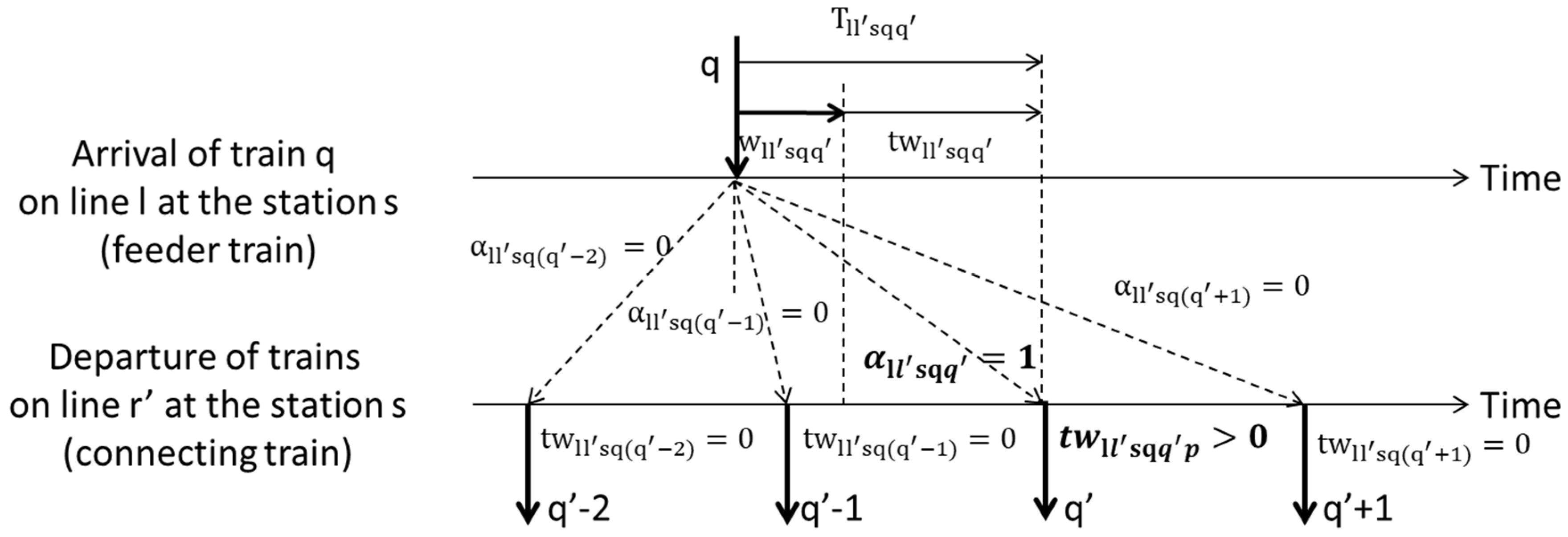
On the basis of these symbols, we use Figure 1 to describe the transfer process and the calculation of transfer waiting time. As shown in this figure, the passengers need to transfer from Line $\mathrm{l}$ to Line ${\mathrm{l}}^{\prime }$, at transfer station$\mathrm{s}$. Transferring to connecting Line${\mathrm{l}}^{\prime }$, passengers need to first walk to the platform. We use the variable${\mathrm{w}}_{{\mathrm{ll}}^{\prime }{\mathrm{sqq}}^{\prime }}$ to present the transfer walking time from the feeder train to the connecting train.

This figure shows the connection relationships among the feeder train $\mathrm{q}$ and a sequence of trains on the connecting line. In order to clarify the relationship between the feeder train and a connecting train, a binary variable, ${\mathsf{\alpha }}_{{\mathrm{ll}}^{\prime }{\mathrm{sqq}}^{\prime }}$, is introduced to describe whether these passengers could transfer from train $\mathrm{q}$ on Line $\mathrm{l}$ to train${\mathrm{q}}^{\prime }$ on Line${\mathrm{l}}^{\prime }$, at station $\mathrm{s}$ successfully. When ${\mathsf{\alpha }}_{{\mathrm{ll}}^{\prime }{\mathrm{sqq}}^{\prime }}$ equals 1 it means the passengers transfer successfully, while ${\mathsf{\alpha }}_{{\mathrm{ll}}^{\prime }{\mathrm{sqq}}^{\prime } }$ equals 0 indicates a transfer failure between train $\mathrm{q}$ on Line$\mathrm{l}$ to train${\mathrm{q}}^{\prime }$ on Line${\mathrm{l}}^{\prime }$, at station $\mathrm{s}$. It is determined based on following formula:

$${\mathsf{\alpha }}_{{\mathrm{ll}}^{\prime }{\mathrm{sqq}}^{\prime }}=\{\begin{array}{c}1,0\le {\mathrm{T}}_{{\mathrm{ll}}^{\prime }{\mathrm{sqq}}^{\prime }}- {\mathrm{w}}_{{\mathrm{ll}}^{\prime }{\mathrm{sqq}}^{\prime }} \le H^T\\ 0, \mathrm{otherwise}\end{array}$$

(1)

In order to determine the value of variable${\mathsf{\alpha }}_{{\mathrm{ll}}^{\prime }{\mathrm{sqq}}^{\prime }}$, the synchronization time, ${\mathrm{T}}_{{\mathrm{ll}}^{\prime }{\mathrm{sqq}}^{\prime }}$, needs to be determined in advance, which is defined as the time gap between the departure time of a connecting train and the arrival time of a feeder train, where ${\mathrm{T}}_{{\mathrm{ll}}^{\prime }{\mathrm{sqq}}^{\prime }}$ is the synchronization time between train $\mathrm{q}$ on Line $\mathrm{l}$ and train ${\mathrm{q}}^{\prime }$ on Line ${\mathrm{l}}^{\prime }$ at station$\mathrm{s}$:

$${\mathrm{T}}_{{\mathrm{ll}}^{\prime }{\mathrm{sqq}}^{\prime }}={\mathrm{D}}_{{\mathrm{l}}^{\prime }{\mathrm{q}}^{\prime }\mathrm{s}}-{\mathrm{A}}_{\mathrm{lqs}}$$

(2)

${\mathrm{T}}_{{\mathrm{ll}}^{\prime }{\mathrm{sqq}}^{\prime }}<0$means that train ${\mathrm{q}}^{\prime }$ on Line ${\mathrm{l}}^{\prime }$ left the station s, before train $\mathrm{q}$ arrived on Line $\mathrm{l}$, for example, train p and train ${\mathrm{q}}^{\prime }-2$, train p and train ${\mathrm{q}}^{\prime }-1$. If the synchronization time ${\mathrm{T}}_{{\mathrm{ll}}^{\prime }{\mathrm{sqq}}^{\prime }}$ is smaller than${\mathrm{w}}_{{\mathrm{ll}}^{\prime }{\mathrm{sqq}}^{\prime }}$, it means this time is not sufficient enough for a passenger to walk to the transfer platform, which is also a transfer failure with the value of ${\mathsf{\alpha }}_{{\mathrm{ll}}^{\prime }{\mathrm{sqq}}^{\prime }}$ as 0. On the contrary, passengers have enough time to transfer to the platform, and the situation exists that passengers prefer to skip trains and board later ones. Here, we assume that all passengers will get on the next possible connecting train and the capacity is sufficient for these passengers. Therefore, only the first possible connecting train is defined as a successful transfer. The values of${\mathsf{\alpha }}_{{\mathrm{ll}}^{\prime }{\mathrm{sqq}}^{\prime }}$are also set to be 0 for late trains. In this example, the synchronization time is not enough for them to walk from the feeder train to train q’- 1. Therefore, the passenger has to wait and get on the following train q’. Therefore, the ${\mathsf{\alpha }}_{{\mathrm{ll}}^{\prime }{\mathrm{sqq}}^{\prime }}$ equals 1 and ${\mathsf{\alpha }}_{{\mathrm{ll}}^{\prime }\mathrm{sq}{({\mathrm{q}}^{\prime }-1)}^{\prime }}$ equals 0.

Meanwhile, the transfer waiting time ${\mathrm{tw}}_{{\mathrm{ll}}^{\prime }{\mathrm{sqq}}^{\prime }}$ is calculated as the synchronization time minus the transfer walking time. Normally, it is positive. If the transfer walking time is negative, it means they did not catch this train, and then we set the value of the transfer waiting time as 0 in this model. The value of the transfer walking time is quite important for transfer passengers. A long transfer waiting time is negative for transfer passengers. Therefore, in timetable synchronization, designers have to reduce the amount of transfer waiting time, where transfer passengers from train q on Line l will take train q’ on Line l’ with a transfer waiting time${\mathrm{tw}}_{{\mathrm{ll}}^{\prime }{\mathrm{sqq}}^{\prime }}$.

2.3. Constraints

In this section, we introduce the basic constraints for the transfer synchronization problem for cross-platform transfer for the whole day, including train operation, headway, just-miss constraints, and so on as follows:

1. Train operation constraints

In this study, we assume that the running time on each section between station s and station s +1 are constant values. Meanwhile, the dwell time on each station s is constant for all trains. These constraints define the arrival and departure time of each train at terminal stations.

$${\mathrm{A}}_{\mathrm{lqs}}={\mathrm{D}}_{\mathrm{lq}0}+{\displaystyle \sum }_{\mathrm{k}=1}^{\mathrm{s}}{\mathrm{R}}_{\mathrm{lqk}}+{\displaystyle \sum }_{\mathrm{k}=1}^{\mathrm{s}-1}{\mathrm{E}}_{\mathrm{lqk}}$$

(3)

$${\mathrm{D}}_{\mathrm{lqs}}={\mathrm{A}}_{\mathrm{lqs}}+{\mathrm{E}}_{\mathrm{lqs}}$$

(4)

Our transfer synchronization model is based on a basic timetable, which is designed based on the time-varying passenger demand. Therefore, the adjustment of departure time at first station on Line $\mathrm{l}$ of this prescheduled timetable is limited to the following range:

$${\mathrm{d}}_{\mathrm{l}}^{\min }\le {\mathrm{ad}}_{\mathrm{lq}}\le {\mathrm{d}}_{\mathrm{l}}^{\max }$$

(5)

2. Safety headway constraints

Enough headway should be guaranteed between consecutive trains on the same station. In addition, in order to guarantee a certain train service frequency, the departure headway should not be too large. Since the headways are set differently for these operational time periods considering passenger requirements, the headway constraints are set for each operation time period as:

$${\mathrm{h}}_{\mathrm{ls}}^{\mathrm{T},\min }\le {\mathrm{D}}_{\mathrm{l}\left(\mathrm{q}+1\right)\mathrm{s}}-{\mathrm{D}}_{\mathrm{lqs}}\le {\mathrm{h}}_{\mathrm{ls}}^{T,\max }$$

(6)

Especially for the transit time period from peak to off-peak or vice versa, the headway between consecutive trains, the headways should be smaller than the headway during an off-peak time period, and bigger than the headway during a peak time period.

3. Train turn-around constraints

This constraint guarantees that each train has enough time to turn their running direction at the turn-around station.

$${\mathrm{ndt}}_{\mathrm{lq}}-{\mathrm{at}}_{\mathrm{lq}{N}_l}\ge {\mathrm{ta}}_{{\mathrm{lN}}_l}^{\min }$$

(7)

4. Just miss constraints

Just miss means that passenger saw the connecting train leaving when they reached the transfer platform, which causes significant passenger dissatisfaction [16]. This influence is more significant for cross-platform transfer, since the transfer passengers can directly see the trains on the opposite track. Therefore, the constraint is set as follows to avoid just miss:

$$A_{lqs}-{\mathrm{D}}_{l^{\prime }{\mathrm{q}}^{\prime }\mathrm{s}}>{\mathrm{CT}}_{\mathrm{ls}}$$

(8)

2.4. Objective

This study aims to minimize the weighted average transfer waiting time in transfer synchronization for the whole day as follows:

$$\min \left\{{\displaystyle \sum }_{\left(\mathrm{l},{\mathrm{l}}^{\prime }\right)}{\displaystyle \sum }_{\mathrm{s}}{\displaystyle \sum }_{\mathrm{q}}{\displaystyle \sum }_{{\mathrm{q}}^{\prime }}{\mathrm{p}}_{\mathrm{l}{\mathrm{l}}^{\prime }{\mathrm{sqq}}^{\prime }}{\ast \mathrm{tw}}_{{\mathrm{ll}}^{\prime }{\mathrm{sqq}}^{\prime }}/{\displaystyle \sum }_{\left(\mathrm{l},{\mathrm{l}}^{\prime }\right)}{\displaystyle \sum }_{\mathrm{s}}{\displaystyle \sum }_{\mathrm{q}}{\displaystyle \sum }_{{\mathrm{q}}^{\prime }}{\mathrm{p}}_{{\mathrm{ll}}^{\prime }{\mathrm{sqq}}^{\prime }}\right\}$$

(9)

where ${\mathrm{tw}}_{{\mathrm{ll}}^{\prime }{\mathrm{sqq}}^{\prime }}$ is the transfer waiting time for transfer pair, from train q on Line l to train q’ on Line l’.

As previously described, the transfer waiting time is 0 if the variable ${\mathsf{\alpha }}_{{\mathrm{ll}}^{\prime }{\mathrm{sqq}}^{\prime }}$ is 0. When a successful transfer is checked with ${\mathsf{\alpha }}_{{\mathrm{ll}}^{\prime }{\mathrm{sqq}}^{\prime }}$ as 1, the transfer waiting time ${\mathrm{tw}}_{{\mathrm{ll}}^{\prime }{\mathrm{sqq}}^{\prime }}$ is calculated by${\mathrm{T}}_{{\mathrm{ll}}^{\prime }{\mathrm{sqq}}^{\prime }}$ minus${\mathrm{w}}_{{\mathrm{ll}}^{\prime }{\mathrm{sqq}}^{\prime }}$:

$${\mathrm{tw}}_{{\mathrm{ll}}^{\prime }{\mathrm{sqq}}^{\prime }}=\{\begin{array}{c}0, {\mathsf{\alpha }}_{{\mathrm{ll}}^{\prime }{\mathrm{sqq}}^{\prime }}=0\\ {\mathrm{T}}_{{\mathrm{ll}}^{\prime }{\mathrm{sqq}}^{\prime }}-{\mathrm{w}}_{{\mathrm{ll}}^{\prime }{\mathrm{sqq}}^{\prime }}, {\mathsf{\alpha }}_{{\mathrm{ll}}^{\prime }{\mathrm{sqq}}^{\prime }}=1\end{array}$$

(10)

The weighted transfer waiting time is the number of transfer passengers for the target transfer pair. In our study, we assume these passengers are evenly distributed.

3. Algorithm

In this research, transfer synchronization was conducted based on a historical timetable and the decision variables are the adjustments of departure times for all trains at their initial stations in this historical timetable. The generic algorithm (GA) is a stochastic heuristic optimization procedure, which is widely applied to solve the NLP (Nonlinear Programming) problem in an urban rail transit system [1, 2, and 3]. In this paper, we designed a GA-based algorithm to solve the proposed model for cross-platform transfer synchronization. The flow chart for this algorithm is shown in Figure 2 and some key operations in the GA are elaborated.

• Chromosome Coding

The adjustments of departure times at the initial station for all trains were chosen as genes for chromosomes using decimal integer coding, denoted as$\left\{{\mathrm{ad}}_{\mathrm{i},1},{\mathrm{ad}}_{\mathrm{i},2},\dots ,{\mathrm{ad}}_{\mathrm{i},{\mathrm{Q}}_{\mathrm{i}}}\right\}$ for each line (with direction), where ${\mathrm{Q}}_{\mathrm{i}}$ presents the total number of trains on Line $\mathrm{i}$. An example for chromosome is shown in Figure 3. In this paper, the down running direction and up running direction of a practical line were treated as different lines in this model. Therefore, in total, four lines (two practical lines with four directions) are defined in the chromosome for a cross-platform transfer.

2.

Population/Individual Initialization

The individuals in the first generation are initialization in this step. Each gene of an individual is initialized with the random value between the lower and upper boundaries defined in Formula (5). When an individual is initialized, we have to check the feasibility, excluding the individual which does not satisfy the constraints. If the initialized individual is unfeasible, return to the step of individual initialization until the number of feasible individuals reaches the predetermined population size.

3.

Fitness function

The fitness value is the original objective function, minimizing weighted transfer waiting time at the transfer station. The fitness function of each individual can be expressed as the following formula:

$$\mathrm{F}={\displaystyle \sum }_{\left(\mathrm{l},{\mathrm{l}}^{\prime }\right)}{\displaystyle \sum }_{\mathrm{s}}{\displaystyle \sum }_{\mathrm{q}}{\displaystyle \sum }_{{\mathrm{q}}^{\prime }}{\mathrm{p}}_{{\mathrm{ll}}^{\prime }{\mathrm{sqq}}^{\prime }}{ \ast \mathrm{tw}}_{{\mathrm{ll}}^{\prime }{\mathrm{sqq}}^{\prime }}/{\displaystyle \sum }_{\left(\mathrm{l},{\mathrm{l}}^{\prime }\right)}{\displaystyle \sum }_{\mathrm{s}}{\displaystyle \sum }_{\mathrm{q}}{\displaystyle \sum }_{{\mathrm{q}}^{\prime }}{\mathrm{p}}_{{\mathrm{ll}}^{\prime }{\mathrm{sqq}}^{\prime }}$$

(11)

This calculation of fitness is based on the timetables of two practical lines associated with the transfer. Therefore, the first step is to generate the modified timetable based on the adjustment of departure time for each train which is recorded in the chromosomes. Then, the calculation process follows Formulas (9)–(10) with timetables, transfer walking time, and time-depend transfer passengers as inputs.

4.

Selection and elitist preservation operator

The selection operator ensures that the optimal individuals are inherited to the next generation. Tournament selection was employed to make the selection, which arranges a tournament between two randomly selected individuals from the population and the individual with better fitness is the winner of the tournament and selected. Comparing to the traditional roulette method, this method improves the evolution rate of the population and maintains the stability of the population.

5

Recombination operator

This paper employs the simulated binary crossover (SBX) operator to recombine the gene of selected parents for the real-coded genetic algorithm, which creates offspring solutions in proportion to the difference in parent solutions [17]. The procedure to find the value of the offspring solution $x_1$ and $x_2$ from parent solutions $p_1$ and $p_2$ is given below:

$$x_1=0.5\left[\left(1+\beta \right)p_1+\left(1-\beta \right)p_2\right]$$

(12)

$$x_2=0.5\left[\left(1-\beta \right)p_1+\left(1+\beta \right)p_2\right]$$

(13)

The separator $\beta$ is defined as the ratio of the absolution difference in children values to the parents:

$$\beta =\{\begin{array}{c}{\left(2u\right)}^{\frac{1}{{\eta }_c+1}}\\ {\left(\frac{1}{2\left(1-u\right)}\right)}^{\frac{1}{{\eta }_c+1}}\end{array}$$

(14)

where $u$ is a random number between 0 and 1 (1 is excluded) and ${\eta }_c$ is the distribution index. A larger ${\eta }_c$ tends to generate offspring closer to the parents. After the recombination, the feasibility of the offspring should also be checked. If the timetable is not feasible, this step will repeat until feasible solutions.

6.

Mutation

The mutation operator can help to avoid local optimal solutions. In this paper, we assume that each individual will have a certain probability of mutation operation, and randomly select the mutation position. Individuals which are mutated randomly, select multiple gene positions for mutation, and randomly select a value within the entire parameter range to replace the original value. To ensure that the new individual still satisfies the constraints, the feasibility of the individual should be checked after mutation. When the individual does not satisfy the constraints, the mutation process will repeat for this individual until the offspring is a feasible timetable.

7.

Elitist preservation operator

Elite selection is utilized in the end in order to guarantee the final results, so that the individual with the highest fitness in each generation is retained, replacing the individuals with the lowest fitness in the next generation.

8.

Termination Criterion

The iteration terminates when the highest fitness is unchanged at a certain number of iterations or the generation reaches the maximum generation, which should be defined in advance.

4. Case Study

In this section, we applied the proposed modeling framework and solution algorithm to the timetable synchronization problem for a real cross-platform transfer scenario in the Beijing urban transit system. The proposed algorithms were coded in Visual Studio C++ 2019, which was performed on a Windows 10 (64-bit) personal computer.

4.1. Case Description and Data Processing

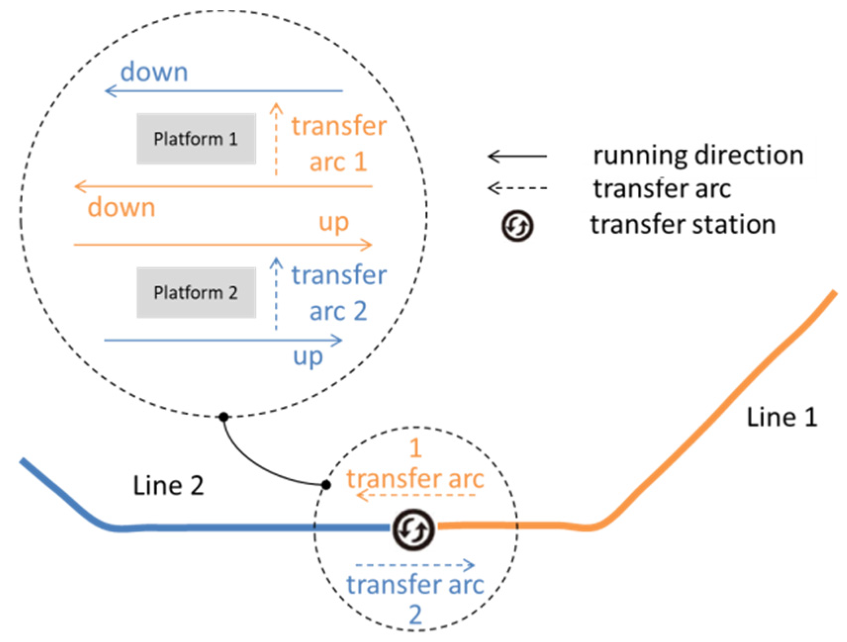
Figure 4 describes the layout of the cross-platform transfer station with two island platforms and four tracks. Line 1 uses the two tracks between two platforms, and Line 2 uses the other two outside tracks. Since this transfer station is a terminal station for the two lines, there are only two transfer directions, named as transfer arc in the figure. The first transfer arc (Transfer arc 1) is that the passengers transfer from Line 1 to Line 2 through Platform 1. The second transfer arc (Transfer arc 2) describes the transfer from Line 2 to Line 1 through Platform 2. The transfer walking time through each island platform is 1 min on average, considering the difference in train length for these two lines.

In Beijing, the design and optimization of timetables are conducted line by line in a certain order based on the characteristics of passenger flow and the network topology in reality. In this case, transfer synchronization was conducted to adjust the departure time and arrival time of trains on Line 2 at the transfer station, coordinating the operation plan on Line 1. These lines are typically commute lines, having an obvious characteristic of tidal flow during peak hours. Taking one normal workday as an example, the total number of passenger flow is 29,182 at the transfer station, where 11,520 passengers transfer from Line 2 to Line 1 and 13,104 passengers from Line 1 to Line 2. These transfer passengers account for a large proportion of all passengers arriving at this transfer station, reaching more than 80%. In addition, almost 50% of the transfer passengers, transfer from Line 2 to Line 1 for work during the morning peak period from 6:30 to 9:00. On the contrary, the main transfer direction is Transfer arc 1 during the afternoon peak period, from Line 1 to Line 2. In addition, therefore, the transfer synchronization is important at this transfer station.

In

Table 1. Headways scheduled for the whole day.

Headway (min)	First Train Period	Morning Peak Period	Morning Off-Peak	Afternoon Peak Period	Afternoon Off-Peak	Last Train Period
Line 1	10	5	8	5	8	10
Line 2	4.5	3	8	4	8	10

, the headways during different time periods of a whole day are described. According to the principle of symmetry operation, the headway during each time period is set the same for both directions. In the transitional period between different time periods, the synchronization of transfer should also be guaranteed. In total, 304 trains are scheduled to run throughout the whole day for Line 2, according to the passenger demand. It should be point out that the departure times of the first and last trains are predetermined by operators and the Beijing Traffic Control Center (TCC) considering the O-D pair of passenger flow in the whole network and it cannot be altered. Therefore, these time points were fixed in the proposed model with a total of 302 variables for this case.

Other model parameters were set based on operational and technical condition of two lines, which is described in detail in

Table 2. Model parameters set for studied case.

Parameter *	Parameter Value
Transfer walking time (s)	60
Trip time for down direction (s)	1310
Trip time for up direction (s)	1285
Train clear time of Line 1 (s)	45
Train clear time of line 2 (s)	45
Minimum turn-round time for down direction (s)	120
Minimum turn-round time for up direction (s)	120
Minimum technical headway (s)	120
Maximum operational headway (s)	900
Time of first train at initial station on down direction (-)	05:30:00
Time of last train at initial station on down direction (-)	22:55:00
Time of first train at initial station on up direction (-)	05:05:00
Time of last train at initial station on up direction (-)	22:30:00

* except train clear time, the other parameters are set for Line 2.

.

For the solution algorithm, the crossover rate is set as 0.7 and the mutation rate is set as 0.005. The population size is 100 and the algorithm will terminate at the 1000th generation or when the fitness value does not change in 100 generations. In addition, a sensitivity analysis of these parameters was also conducted in this case study.

4.2. Results Analysis

Figure 5 presents the optimization results of a single run, which illustrates the optimization progress of best fitness value and mean fitness value in each generation. The X-axis represents the generations of population and the Y-axis represents the best fitness value and the average fitness value in each generation. The result shows that the average weighted transfer waiting time between Line 1 and Line 2 was reduced to 132 s per person for the whole day through 1000 iterations. Compared with the original timetable, the average weighted transfer waiting time is reduced by 20%, from 193 s to 132 s by the proposed model and algorithm. It can be found that the best fitness value reduces more quickly at the initial period. Comparatively, the decrement of best fitness value is gentler in the later period. At the same time, the whole population has better performance with a smaller mean fitness value.

The operational performance of the original timetable and the optimized timetable were also compared in this study, with regards to the following scenarios: just-miss transfer, average transfer waiting time for each transfer pair, and weighted average transfer waiting time per person for the whole day. A comparison of Transfer arc 1 and Transfer arc 2 was completed. As shown in

Table 3. Operational performance of the original timetable and the optimized timetable.

Timetable		Just-Miss Transfer (-)	Average Transfer Waiting Time (s)	Average Weighted Transfer Waiting Time (s0
Original timetable	Transfer arc 1	23	273.08	212.35
	Transfer arc 2	16	211.47	204.17
Optimized timetable	Transfer arc 1	0	138.78	132.58
	Transfer arc 2	0	138.78	132.58

, just-miss transfer scenarios were avoided in the optimized timetable, which effectively improved the trip experience of transfer passengers. In addition, the optimization function average weighted transfer waiting time per person, and also the average transfer waiting time for each transfer pair was generally reduced in the optimized timetable.

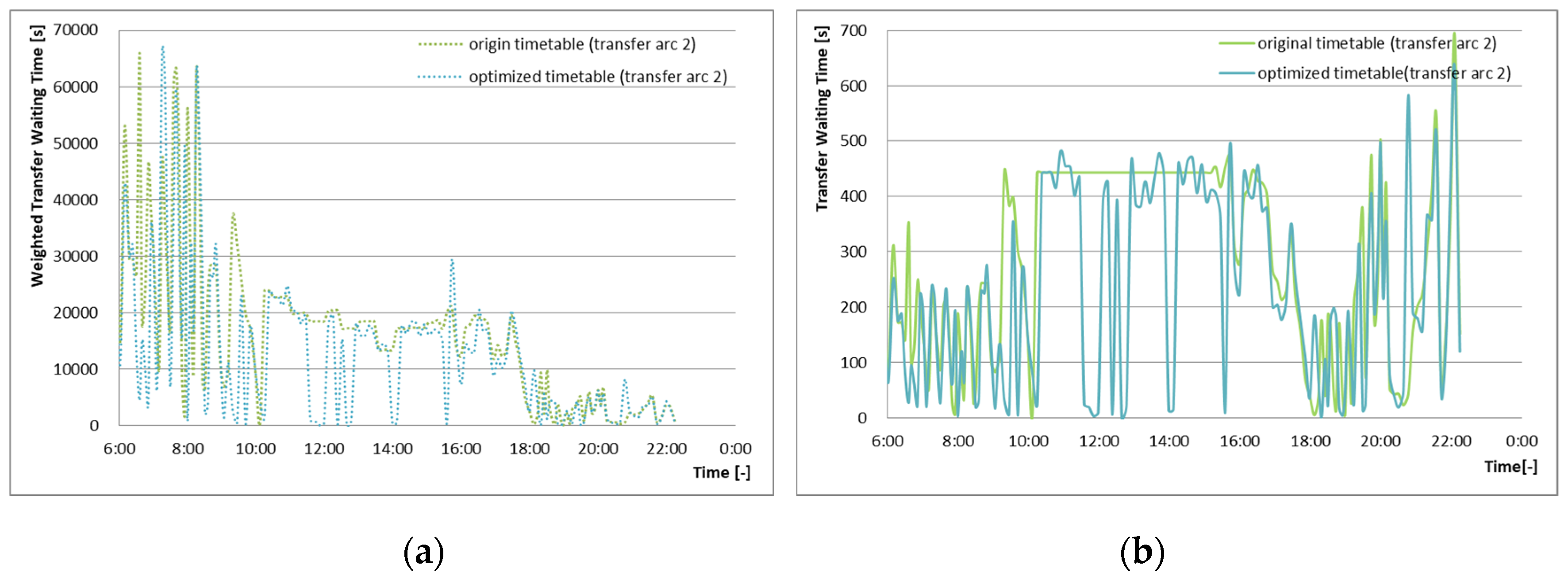
The weighted transfer waiting time considering the amount of passenger flow and the pure transfer waiting time for each transfer pair are both generally reduced in the optimized timetable, as shown in Figure 6. However, there are some exceptions indicating higher weighted transfer waiting times and transfer waiting times for certain transfer pairs, due to the strict constricts described in Section 2.3. We found that the peak weighted transfer waiting time is reached during the afternoon peak period due to the concentrated passenger flow. This peak corresponds to the trial characteristic of passenger flows. The curve in Figure 6b shows the transfer waiting time for each transfer pair in Transfer arc 1. The reduction in transfer waiting time was limited during the time period from 12:00 to 16:00, when the scheduled headways are the same for Line 1 and Line 2. Due to the constraints regarding the operation constraints, turn-around constraints, and just-miss constraints, the adjustment is limited. By comparison, better optimization effects happen during other time periods.

A detailed performance analysis was also done for Transfer arc 1 at this transfer station. Different from the optimization results of Transfer arc 1, there is no general reduction in weighted transfer waiting times and transfer waiting times for all transfer pairs, as shown in Figure 7. However, some certain transfer pairs have huge reductions of weighted transfer waiting time and transfer waiting time as compared with the original timetables, because the optimized timetable avoids several just-miss scenarios through optimization considering the constraints. For this transfer direction, the peak weighted transfer waiting time occurs during the time period from 6:00 to 8:00, when a large number of passengers transfer from Line 2 to Line 1 for work.

For the genetic algorithm, the parameter crossover rate and mutation rate are quite significant for the whole algorithm, which should be determined primarily. In order to obtain a suitable setting of these parameters, some trials should be carried out to test the model for different settings of these parameters. In our model, the population size and maximum generation number are set as 100 and 1000, respectively. We set crossover probability as 0.5, 0.6, 0.7, and 0.8, and mutation probability as 0.005, 0.01, 0.02, and 0.03. Hence, there are 16 kinds of situations in total. We tested every situation five times and the corresponding results are shown in

Table 4. Optimization results for parameter scenarios.

$({\mathit{P}}_{\mathit{C}},{\mathit{P}}_{\mathit{m}})$	Weighted Average Transfer Waiting Time (s)
	1	2	3	4	5	Average
(0.5, 0.001)	133.6046	131.5924	132.8749	132.8528	132.4779	132.6805
(0.5, 0.005)	132.0606	132.1766	131.3146	131.9489	131.4251	131.7852
(0.5, 0.01)	134.9172	135.2101	134.6301	135.4745	134.1522	134.8768
(0.5, 0.02)	138.6853	139.9563	140.3819	140.4382	140.0707	139.9065
(0.5, 0.03)	144.7713	144.2474	143.5480	145.8360	142.2524	144.1310
(0.6, 0.001)	132.1175	133.2350	132.9381	132.3212	132.3879	132.5999
(0.6, 0.005)	131.6824	131.6663	131.5824	131.5753	131.9280	131.6869
(0.6, 0.01)	135.2351	134.5462	135.2084	135.4091	134.8768	135.0551
(0.6, 0.02)	139.2688	141.1980	140.2803	139.2443	139.6086	139.9200
(0.7, 0.001)	133.3183	132.9052	133.9585	132.8812	132.1245	133.0375
(0.7, 0.005)	132.0622	131.2538	131.2728	131.6680	131.5487	131.5611
(0.7, 0.01)	135.0258	134.8982	135.8670	135.9954	133.9305	135.1434
(0.7, 0.02)	137.4536	139.6581	139.894	139.6751	140.3899	139.4141
(0.8, 0.001)	134.7905	134.0476	133.3393	133.1477	132.7718	133.6194
(0.8, 0.005)	131.6352	132.0475	132.2510	131.6513	131.9601	131.9090
(0.8, 0.01)	135.8541	134.7069	134.7013	134.5917	135.6755	135.1059

. In this table, the optimal average fitness value can be obtained with the scenario (0.7, 0.005) as 131.5611 s per person. On the basis of these results, the crossover probability is set as 0.7 and mutation probability is set as 0.005 eventually in this study.

5. Conclusions and Future Research

Considering the change of passenger demands and the utilization of trains throughout the whole day, a mixed integer linear programming model is developed to solve the transfer optimization problem for cross-platform transfer. With the developed model and method, an optimized timetable with less transfer waiting time was obtained by synchronizing the existing timetable. In addition, the transfer optimization could be conducted quickly and coped with the change of timetable in the transfer relationship. This highly improves the efficiency of timetable scheduling in reality. The case study shows that the synchronized timetable for the whole day provides a smoother transfer reducing the transfer waiting time significantly.

There are several improvements that should be done in future research. In a real metro operation, running time and dwell time are assigned for different trains and different time periods in some cases. Therefore, in future research, the adjustment of running time and dwell time would also be considered in modeling the transfer optimization problem to improve the inherent flexibility of this model. In this case, the passenger flow is below the train capacity constraint. However, integrating the train capacity constraint into the transfer optimization model is quite important for extremely busy lines, especially during rush hours. This point should also be considered in future work. In addition, the transfer synchronization problem should also be solved for other types of transfers in order to improve the applicability, such as channel transfer and hall transfer.

References

- Mohring, H.; Schroeter, J.; Wiboonchutikula, P. The Values of Waiting Time, Travel Time, and a Seat on a Bus. RAND J. Econ. 1987, 18, 40. [Google Scholar] [CrossRef]
- Jansen, L.N.; Pedersen, M.B.; Nielsen, O.A. Minimizing Passenger Transfer Times in Public Transport Timetables. In Proceedings of the 7th Conference of the Hong Kong Society for Transportation Studies: Transportation in the Information Age, Hong Kong, China, 14 December 2002; pp. 229–239. [Google Scholar]
- Ye, Y.; Zhang, J.; Wang, Y. Transfer Coordination-Based Train Organization for Small-Size Metro Networks. Arab. J. Sci. Eng. 2019, 45, 3599–3610. [Google Scholar] [CrossRef]
- Chakroborty, P. Genetic Algorithms for Optimal Urban Transit Network Design. Comput. Civ. Infrastruct. Eng. 2003, 18, 184–200. [Google Scholar] [CrossRef]
- Yin, H.; Wu, J.; Sun, H.; Kang, L.; Liu, R. Optimizing last trains timetable in the urban rail network: Social welfare and synchronization. Transp. B Transp. Dyn. 2018, 7, 473–497. [Google Scholar] [CrossRef]
- Teodorović, D.; Lucic, P. Schedule synchronization in public transit using the fuzzy ant system. Transp. Plan. Technol. 2005, 28, 47–76. [Google Scholar] [CrossRef]
- Cevallos, F.; Zhao, F. Minimizing Transfer Times in Public Transit Network with Genetic Algorithm. In Transportation Research Record. J. Transp. Res. Board 2006, 1971, 74–79. [Google Scholar] [CrossRef]
- Fang, X.; Zhou, L.; Xia, M. Research on Optimization of Urban Mass Transit Network Schedule Based on Coordination of Connecting Time Between Different Lines. In Proceedings of the 2010 Joint Rail Conference, Volume 1, ASME International, Urbana, IL, USA, 12–14 April 2010; pp. 465–477. [Google Scholar]
- Wong, R.C.W.; Yuen, T.W.Y.; Fung, K.W.; Leung, J.M.Y. Optimizing Timetable Synchronization for Rail Mass Transit. Transp. Sci. 2008, 42, 57–69. [Google Scholar] [CrossRef]
- Shafahi, Y.; Khani, A. A practical model for transfer optimization in a transit network: Model formulations and solutions. Transp. Res. Part A Policy Pr. 2010, 44, 377–389. [Google Scholar] [CrossRef]
- Wu, J.; Liu, M.; Sun, H.; Li, T.; Gao, Z.; Wang, D.Z. Equity-based timetable synchronization optimization in urban subway network. Transp. Res. Part C Emerg. Technol. 2015, 51, 1–18. [Google Scholar] [CrossRef]
- Guo, X.; Sun, H.; Wu, J.; Jin, J.; Zhou, J.; Gao, Z. Multiperiod-based timetable optimization for metro transit networks. Transp. Res. Part B Methodol. 2017, 96, 46–67. [Google Scholar] [CrossRef]
- Guo, X.; Wu, J.; Sun, H.; Liu, R.; Gao, Z. Timetable coordination of first trains in urban railway network: A case study of Beijing. Appl. Math. Model. 2016, 40, 8048–8066. [Google Scholar] [CrossRef]
- Kang, L.; Wu, J.; Sun, H.; Zhu, X.; Wang, B. A practical model for last train rescheduling with train delay in urban railway transit networks. Omega 2015, 50, 29–42. [Google Scholar] [CrossRef]
- Zhou, W.; Deng, L.; Xie, M.; Yang, X. Coordination Optimization of the First and Last Trains’ Departure Time on Urban Rail Transit Network. Adv. Mech. Eng. 2013, 5, 848292. [Google Scholar] [CrossRef]
- Kwan, C.M.; Chang, C. Timetable Synchronization of Mass Rapid Transit System Using Multiobjective Evolutionary Approach. IEEE Trans. Syst. Man, Cybern. Part C Applications Rev. 2008, 38, 636–648. [Google Scholar] [CrossRef]
- Deb, K.; Agrawal, R.B. Simulated binary crossover for continuous search space. Complex Syst. 1995, 9, 115–148. [Google Scholar]
© 2020 by the authors. Licensee MDPI, Basel, Switzerland. This article is an open access article distributed under the terms and conditions of the Creative Commons Attribution (CC BY) license (http://creativecommons.org/licenses/by/4.0/).