Article

Applied Identification of Industry Data Science Using an Advanced Multi-Componential Discretization Model

1
Department of Information Management, Hwa Hsia University of Technology, New Taipei City 23568, Taiwan
2
School of Computing Science and Engineering, VIT University, Vellore 632014, Tamil Nadu, India
3
National Museum of Marine Science & Technology, Keelung City 202010, Taiwan
*
Authors to whom correspondence should be addressed.
Symmetry 2020, 12(10), 1620; https://doi.org/10.3390/sym12101620
Submission received: 11 August 2020 / Revised: 14 September 2020 / Accepted: 16 September 2020 / Published: 30 September 2020
(This article belongs to the Special Issue Recent Advances in Social Data and Artificial Intelligence 2019)

Abstract

:
Applied human large-scale data are collected from heterogeneous science or industry databases for the purposes of achieving data utilization in complex application environments, such as in financial applications. This has posed great opportunities and challenges to all kinds of scientific data researchers. Thus, finding an intelligent hybrid model that solves financial application problems of the stock market is an important issue for financial analysts. In practice, classification applications that focus on the earnings per share (EPS) with financial ratios from an industry database often demonstrate that the data meet the abovementioned standards and have particularly high application value. This study proposes several advanced multicomponential discretization models, named Models A–E, where each model identifies and presents a positive/negative diagnosis based on the experiences of the latest financial statements from six different industries. The varied components of the model test performance measurements comparatively by using data-preprocessing, data-discretization, feature-selection, two data split methods, machine learning, rule-based decision tree knowledge, time-lag effects, different times of running experiments, and two different class types. The experimental dataset had 24 condition features and a decision feature EPS that was used to classify the data into two and three classes for comparison. Empirically, the analytical results of this study showed that three main determinants were identified: total asset growth rate, operating income per share, and times interest earned. The core components of the following techniques are as follows: data-discretization and feature-selection, with some noted classifiers that had significantly better accuracy. Total solution results demonstrated the following key points: (1) The highest accuracy, 92.46%, occurred in Model C from the use of decision tree learning with a percentage-split method for two classes in one run; (2) the highest accuracy mean, 91.44%, occurred in Models D and E from the use of naïve Bayes learning for cross-validation and percentage-split methods for each class for 10 runs; (3) the highest average accuracy mean, 87.53%, occurred in Models D and E with a cross-validation method for each class; (4) the highest accuracy, 92.46%, occurred in Model C from the use of decision tree learning-C4.5 with the percentage-split method and no time-lag for each class. This study concludes that its contribution is regarded as managerial implication and technical direction for practical finance in which a multicomponential discretization model has limited use and is rarely seen as applied by scientific industry data due to various restrictions.

1. Introduction

Stock investments may earn profits but are often associated with inherent risks. That is, risks in terms of a stock are a part of financial investments. Stock investors typically face specific risks, such as systematic risk or undiversifiable risk (such as economic risks or inflation), unsystematic risk or idiosyncratic risk (such as market value risk, interest rate risk, and commodity risk), and others (e.g., opportunity risk and liquidity risk) in dealing with the major problems caused by economic and noneconomic factors. Thus, learning about the risk of making appropriate decisions to meet financial goals is an ongoing and important issue. In particular, escaping risks caused by economic uncertainty for stock investments has the following characteristics: dynamism and cyclicality, both of which form a focal and widely studied topic as they make a significant impact on the profitability of financial investments to the stock investors. Financial investments have attracted much attention because investors invest in the stock market, which results in various researchers using data to explore money markets [1] by achieving good data utilization in complex financial industry environments, such as through the use of smart/intelligent models or techniques. Therefore, this study is focused on financial applications with big data solutions that trigger advanced and intelligent componential models. These have posed great opportunities and challenges for data researchers because applied large-scale data are collected from diversified database services in a mixed-industry setting.
Within big data technology communities, large-scale data are collected from heterogeneous network services and integrated for good data utilization that addresses real-world problems. Technological advancement in financial management has been affected by the big data paradigm, such as the application of data mining to manage stock investments. Stocks with distinct characteristics in major markets have been a popular tool for analysis for investment purposes in Taiwan. Based on the data from the Taiwan Stock Exchange (TWSE), up to August 2015, the accumulated number of accounts opened was 17,771,994, and the number of accumulated investors with trading accounts was 9,715,629, while the population of Taiwan was just 23.51 million. Obviously, this shows active and busy market trends. Stock selection is a real-world problem because there are over 880 listed companies. It is a complex and risky issue to choose TWSE stocks. The measures used some main components that were unsystematic and had other risks involved in investing in stocks, such as commodity risk, currency risk, equity risk, headline risk, interest rate risk, obsolescence risk, or legislative risk, among which commodity risk is specific to the risk in connection with fluctuating commodity prices, such as copper, gold, or oil. Commodity risk is highly correlated with natural hazards; this allows it to be analyzed and managed with intelligent information from data mining [2,3]. Some advances in data mining technology (such as by Wang and Miao [4]) applied in stock analysis can definitely assist in escaping risk and achieving better investment performance. Thus, effective analytical tools or techniques are a priority to achieve the goals stated above. The principles of stock analysis have the following routes: technical analysis and fundamental analysis, which are used to prevent investors from searching for suitable research material on the stock market and are employed objectively and scientifically in modeling classification activities and functions for this study, as follows.
(1) Technical analysis: It is the knowledge and steps used to assess stocks to predict future trends by measuring the statistics collected from stock trading activities, such as price or volume changes. Technical analysts indicate that the past trading activity of a stock, in terms of price and volume changes, is a good sign for possible future price trends. First, market prices may offer rebates for various factors that affect the stock price. Second, market price trends or movements are not random but specific trends or movements of an identified pattern. Over the past decade, commonly used indicators include price trend indices, such as varied types of the moving average (MA) [5] or momentum indices, such as moving average convergence and divergence (MACD) [6]. MA has an average of closing prices of a specific number of time periods, such as a 7-period MA for seven days, which defines a flowing correlation between the time period and the money rate [5]. MACD uses exponential moving averages (EMAs) to calculate its value, equal to the value of the shorter time of EMAs and less than the value of the longer time of EMAs [7]. Furthermore, many varied and diverse perspectives for MA and MACD were studied for these purposes, such as EMA, simple moving average (SMA), or weighted moving average (WMA), and variety of MACD-1–4 [7]. These are suitable for stock predictions, as shown in recent studies that demonstrated good performance and were involved in risk aversion.
(2) Fundamental analysis: It is the knowledge and steps of assessing a stock to estimate its intrinsic value by way of measuring related financial, economic, and other quantitative or qualitative attributes. Fundamental analysts study something that may affect stock value, such as the overall industry and economic qualifications of macroeconomic conditions. Its main purpose is highlighted to calculate a quantifiable value for an investor to measure its price at a specific time and to evaluate whether that stock is over- or undervalued. The fundamental analysis utilizes earnings, future growth, profit margins, return on equity, and revenues, among others, as evaluation instruments for stocks and equities because they identify a company’s underlying value and future potential for growth. In particular, fundamental analysis reads a company’s financial statements in terms of the company as a stock. A company’s value is measured by its ability to realize cash flow under uncertainty; at the same time, it is the measure of modern finance to assess asset value, which is defined as being equal to the present value of the expected future cash flow since it is always discounted at the indispensable return. Three variables for its valuation models, including discounted cash flow models (DCFMs), dividend discount models (DDMs), and models depend on multiples (MDMs), are defined. First, DDMs make an elementary assumption, i.e., the value of a stock is decided by rebating the anticipated dividend as future cash. Therefore, the real value of a stock is decided by the present value of the stock cash dividend, which will be received by the shareholder. However, if the company chooses to reduce or stop dividends, the formula of DDMs becomes unworkable. Second, DCFMs were developed as an alternative. In DCFMs, analysts calculate the free cash flow of the company, consider the tax, depreciation, and amortization, change in working capital and capital expenditure, and discount the terminal value and free cash flow to gain the intrinsic value of a company. Third, compared to DDMs and DCFMs, more commonly used are the multiples that determine stock value. Such multiplier models (i.e., MDMs) assume that the company’s value is several times the earnings, sales, cash flow, or book value. For example, referring to the earning multiplier model, the stock value is equal to multiple times the earnings. The information implies that the stock price is exactly several times its earnings per share (EPS) [8]. EPS is served as a financial indicator for the portion of earnings per outstanding share of allocated common stock for a company’s profit over a fixed period of time [9,10]. The same logic applies to book value per share, cash flow per share, and sales per share to form variation of multiplier models. Among these models, company earnings are the most commonly used practical information. Estimating EPS is particularly crucial to analysts of fundamental analysis for complicated financial data. Moreover, as the market is developing and becoming more efficient, fundamental analysis is receiving more attention in the long-term. Given the above reasons, the EPS of fundamental analysis is emphasized in this study due to its preeminent advances and rich features.
Fundamental analysis is used to analyze data from financial reports, which assumes that the market price of a stock is centered on the company’s intrinsic value. With further regard to financial reports, financial statements [11,12] should be addressed preferentially and contiguously to reflect a company’s performance, such as an income statement, balance sheet, and a statement of cash flow. This study proposes advanced multicomponential discretization models that will analyze and mine data about financial ratios by predicting EPS. High EPS for fundamental analysis is the core selection used by investors to buy or hold a stock for a longer period of time. Classification applications for EPS from data from industry databases are of high practical value. Finding an intelligent hybrid classification model that develops out of financial ratio applications is considered an important issue for financial analysts. Many advanced componential data mining techniques used in this study are focused on some effective tools, such as data-discretization, feature-selection, and classification methods. Their performance is assessed and verified by looking at the application of financial ratios versus motivations by proposing an advanced multitechnological use for data processing analytics.
The main purpose of this study is as follows: (a) To build hybrid classification models using an advanced computing framework to diagnose and classify EPS from views of fundamental analysis and to evaluate their effectiveness; (b) to use the paths of literature review and relevant expert knowledge to select the essential financial ratios in advance; (c) to measure various multicomponent discretization performances of the applied hybrid models proposed; (d) to evaluate various classifiers’ performance arising from big data recorded from the stock market to establish the identification of a specific target picture; the financial diagnosis application of comparative studies uses classifiers of advanced noted machine learning (ML) computing, such as the K-nearest neighbor (KNN) algorithm, decision tree (DT) learning, ensemble learning of stacking (STK), radial basis function network (RBFN), and naïve Bayes (NB) due to their past superior performance [11]; (e) to identify effective financial ratios useful to address EPS issues; (f) to discretize the selected condition attributes into corresponded linguistic terms of natural language; (g) to generate the knowledge of comprehensible decision tree-based rules extracted from the given datasets; (h) to identify suitable alternative work available for further research and use a difference-oriented exploration from the rich information.
As a whole, Section 2 introduces the literature to review relevant financial ratio issues. Section 3 presents the main framework of the study methods and materials used. Section 4 describes the data experiments and data analyses executed from the collected dataset, and Section 5 forms a complete discussion. Finally, Section 6 makes some conclusions and talks about future research.

2. Literature Review

The section discusses relevant issues for the identification of financial EPS diagnosis as well as some ML computing approaches, such as the applied financial ratio from scientific data, decision tree learning, the K-nearest neighbor algorithm, applied ensemble learning of stacking, the radial basis function network, and applied naïve Bayes.

2.1. Applied Financial Ratio from Scientific Data

From the perspective of fundamental analysis, financial ratios [13,14,15,16] are helpful to better understand the overall information of a specific company and its operating performance for various kinds of benefits. They are a premotivator to determine the company’s financial condition from financial statements, and, in particular, they are used for comparisons for stakeholders, such as a company’s owner and current and potential investors, in various object-oriented interpretations. Regarding the purposes of comparisons and analyses, financial ratios are measured between similar or competitive countries, industries, and companies, within different time ranges for one company or within a company with an industry-average and with benchmarked objects. Examples of financial ratios are often categorized into five specific groups, including debt ratios, market value ratios, profitability ratios, solvency ratios, and turnover ratios [14], and in most instances, quantify different aspects of a specific company from static and dynamic viewpoints. Mainly, (1) debt ratios are the measurement of the efficiency to refund previous long-term debt and the availability of using cash to return debt; (2) market value ratios value the investment return for shareholders and concern the response to return and the cost of issuing stock; (3) profitability ratios are used to assess the efficiency of using assets to manage operation performances for gaining an acceptable rate of earnings during a specific time period; (4) solvency ratios used are to evaluate the liquidity for uncashed assets converted into cash assets; (5) turnover ratios are used to measure operation ability by using owner assets to produce operating sales, and, in particular, they are valuable mediators in illustrating the operation performance of a company. Values of financial ratios used are calculated from various financial statements, such as the statements of balance sheet, income, cash flows, and the changes in equity [17]. As for most of these ratios, the value of the ratios improves with the performance that the company has compared with its competitors’ ratio or a similar ratio with a specific time interval. Thus, financial ratios are of great interest to potential shareholders of a company, creditors, and financial managers to compare the SWOT (strengths, weaknesses, opportunities, and threats) analyses of various companies.
In practice, financial ratios are associated with predictive factors to EPS from the stock market. A study highlighted 20 key financial ratios that are known to be more relevant with EPS because they are considered to be highly correlated by financial experts and have had a limited literature review in earlier studies [9,11,12]. They are the accounts receivable turnover ratio, cash flow of each share, cash flow ratio, cash ratio, current liabilities, current ratio, debt ratio, fixed asset turnover ratio, interest expense, inventory turnover ratio, net asset value of each share, net worth turnover ratio, operating income per share, operating income margin, quick ratio, return on net asset, sales per share, times interest earned, total asset turnover ratio, and year-on-year percentage total assets, and they are grouped into five financial categories.

2.2. Decision Tree Learning

As to ML algorithms, DT learning [18] is a prominent classification method commonly used in data-mining domains that are specifically for multicriteria decision analysis, operations research in decision analysis, operations management, resource costs, and utility functions, which are faced in practical problems, and its main intent is to frame a tree-structured graph representation that predicts the value of a specific attribute from some input attributes. This tree-structured model, in which the specific attribute creates a possibly finite set of target values, is made as a classification decision-tree. The tree-like flowchart model in decision analysis involves three types of internal nodes that denote a test on a variable completely, branches that refer to the outcome of this test, and leaves that denote a decision-labeled class. The routes for root to leaf are linearized as decision-rules of classification, where the outcome is the contents of the leaf nodes. The decisional rules are generalized and formulated as a meaningful type of a comprehensive set like “IF condition 1 and condition 2 and condition 3 … THEN outcome 1”. Algorithms used for constructing DTs [19] usually work top-down in a flowchart-like construction by picking an attribute from each step to best break up the set of decision rules to help identify a better choice that is most likely to achieve a specific goal.
DTs have five major advantages, including (1) they are simple and easy to comprehend and definable in a concise explanation based on DT rules; (2) they use a white box model; (3) they are helpful to determine new possible scenarios; (4) they give values with little hard data; (5) they easily combine with other algorithms in ML techniques. Importantly, C4.5 [20] is used as a core algorithm to create a classification decision rule. It is a popular classifier with a better frequentation within numerous data-mining techniques than the other four DT algorithms, including C5.0, CART (classification and regression trees), CHAID (chi-square automatic interaction detector), and ID3 (iterative dichotomizer 3) [20].

2.3. K-Nearest Neighbors Algorithm

Regarding the field of pattern recognition for ML search processing, the instance where the specific class is projected to be a target class of the closest to training examples is made up as the nearest-neighbor algorithm; for deep definition, a K-nearest neighbor (abbreviated as KNN) algorithm [21] uses a nonparametric approach for important regression analysis and interested classification works. Within the classification stage, K is defined as a constant by the user, and an unlabeled vector is targeted by allocating the label, which has the most frequent use among these K training examples and is nearest to the query point. That is, an objective target is labeled by voting on the plurality of its neighbors and being allocated the target object to the most common class among the KNNs [22,23]. However, the majority voting mechanism occurs with a drawback when facing a skewed class distribution problem. To solve this problem, one way of weighting the classification [24] is by considering the distance calculated from the test light to each of the KNNs. Thus, for both cases of classification and regression tasks, KNN is helpful and useful [23] to set weights from the dedications of the neighbors, which results in the closest neighbor having more contributions compared to the average value than the more remote ones. Specifically, if K = 1, this object is directly dispatched to the class of the single nearest neighbor, and the selection of the best K is highly dependent on the given data [22,25]; although larger K-values lower the noise effect when processing the classification [26], they create less distinction for the boundaries from classes. Interestingly, good Ks are achieved through some heuristic learning approaches, and the performance evaluations (accuracies) of the KNN algorithm are significantly distorted and degraded by the irrelevant features and the presence of unexpected noise. Efforts for scaling and selecting features from many researchers have been improved with classification performance. Thus, an interesting and popular tool uses the reciprocal information [27] on the data with the classes trained and the evolutionary algorithms to optimize feature selecting and scaling. In particular, the output is a class membership in KNN’s classification community.
Conversely speaking, KNNs have some disadvantages with larger sets of data as they are computationally intensive and tractable. In particular, KNNs are an instance-based heuristic learning method; the effects are locally approximative, and all mathematical computations are postponed until the classification work is complete [28]. The classification performance of KNNs is always significantly improved through supervised learning techniques, resulting in some strongly consistent results. Some algorithms for nearest neighbors have been intensively studied during the past decades, and this research has focused on seeking a decrease in all numbers of distance assessments actually fulfilled. Given the case, it is possible to make great improvements to the speed of KNNs by using proximity graphs [28].
KNN algorithms are the simplest type of algorithm for ML communities, where its algorithms are easier to perform by calculating the distances from all the test examples to the stored examples. Given these successful reasons for using the KNN algorithm in the context of various application data, the classification performance of KNNs will be increased effectively and significantly if the distance metric is studied and learned by a specialized algorithm like the large margin nearest neighbor (LMNN) classification algorithm [29]; the KNN algorithm is analyzed extensively [30] in this study to seek its performance in classification learning.

2.4. Applied Ensemble Learning of Stacking Classifier

Regarding the introduction of ML techniques, an ensemble method is important for conducting an empirical exploration. The ensemble method, which produces more accurate solutions, uses several learning algorithms to construct a new classifier [31,32] in unsupervised and supervised learning cases; it is called a meta-algorithm. Although this ensemble classification method tends to achieve empirically more predictive outcomes when a major variation between these models is faced and shows more flexibility functions [33], the prediction of this ensemble method needs more computational time than the prediction of a stand-alone model. Thus, ensemble methods are regarded as a way to perform extra computations to compensate for poor search-learning algorithms. There are various types of ensemble learning classification approaches [34] (that is, stacking, bagging, and boosting), and there is no single winner. First, bagging has a function to reduce the variation from the prediction by using a repetition method for adding data from the original dataset for training. Second, boosting adopts a two-step procedure to use subsets from the raw data to yield, on average, a series of carrying-out classification systems and boosts their classification performance by using a particular method of majority voting to unite them. Third, stacking [35] (STK) is a similar boosting method, and what is unique is that STK is able to determine the models constructed. In particular, it trains a learning model of such an ensemble method to make the predictions of combining other learning models to the STK classifier. Interestingly, a logistic regression algorithm is more used for the combiner in the STK method. STK [36] typically yields better performance than any of the stand-alone models trained, and it is well made for some supervised learning algorithms, such as regression analysis [37] and the classification method [38] and unsupervised learning algorithms such as chemical process fault diagnosis [39].
Although the performance that combines a variety of strong hybrid learning algorithms [40] to promote diversity is more effective than using single models, it is difficult to apply this method to find the best approach for overcoming practical problems. Theoretically, the STK algorithm [41] yields better classification performance than any single one of the models trained. Thus, the performance of the STK algorithm is tested in practice in this study.

2.5. Radial Basis Function Network

Typically, the radial basis function network [42] (RBFN) is used for the construction of an algorithm of a type of artificial neural network (ANN), which gives radial basis algorithms the role of an activation function in forming a mathematical model that is helpful in defining linear problems of functioning inputs and neuron parameters. RBFNs have three layers of structure, including a pass-through input layer, a hidden layer, and an output layer. Regarding the formation of the layers’ structure, the input layer is formed for a vector of realistic numbers and is linked to a number of hidden neurons, and the Euclidean distance for a center vector and a Gaussian function [42] is typically used in the norm formulation since the function is radially symmetric to this vector; thus, the radial basis algorithm is named. RBFNs consider different natures of the nonlinear hidden neurons versus the linear output neuron and are justified by weights. RBFNs are processed in a two-step algorithm corresponding to the training done. The first step involves performing unsupervised learning to choose and fix the center vectors, width, and weights in the hidden layers. The center vectors are defined by using a K-means clustering algorithm, or they are sampled and trained randomly from some sets of instances since no obvious way is effectively determined for the centers. Interestingly, RBFN is a type of nonparametric model, and its weights with parameters do not have a special intention associated with the problem to which it is used for estimating the values of a neural network in supervised learning [43,44]. The second step simply involves fitting a linear model with appropriate weights to create the hidden layer’s output based on some objective function, such as the least-squares function that optimizes the accuracy of fit by the optimal choice of weights [45].
A main advantage of the RBFN is to keep the mathematics model simple. RBFN is relatively cheap in linear algebra and computational intelligence [43]. In particular, RBFN learns how to convert input data to a wanted response, and it has widely used for the functions of pattern recognition, classification, time series prediction, system control, and approximation [46,47,48]. The above rationality for the noticed well-being of the RBFN classifier in previous research is highlighted within this study; it is selected as one of the primary goals of complex comparison purposes to estimate the underlying function of neural networks due to their intrinsic meaning.

2.6. Applied Naïve Bayes

In applied views of ML domains, the classifier of naïve Bayes, NB, is a popular approach in a simple type of probabilistic process of classifier, with powerfully independent hypotheses between the attributes to process real-life problems according to Bayes’ theorem [49,50]. NB assumes that the value of a specific attribute has independence from the value of any other attributes in the class variable given, and it effectively considers each of the attributes to be independently devoted to the possibility used. In spite of the naïve design and oversimplified hypotheses, the NB classifier [51,52] has done well, with considerable applications for complex real-world problems, particularly in financial prediction and medical diagnosis, with more advanced computing methods. From the limited literature on statistics and computer science, the NB classifier holds many capabilities that make it helpful enough to attract the attention of researchers. First, for completing the decoupling of the class distributions of conditional features, each distribution is estimated independently for a type of one-dimensional distribution, which serves to lessen a real problem derived from the effects of the curse of dimensionality on dataset features. Second, in many real applications, the method of maximum likelihood is used as an extensive parameter estimation for NB classification models; restated, it is unnecessary to accept Bayesian probability or to use any Bayesian method. Third, the NB classifier [53] of ML is highly concerned with scalable jobs in some linear parameters for the attributes used for solving real-life problems.
According to a smart advantage of NB [54], only small numbers of data training are needed to produce a good forecast of the linear parameter that is useful to classification works in many applications in order to meet the requirement of a good classifier. Given this reason, the classifier is sound enough to neglect strict inadequacy in the fundamental naïve probabilities of models. Regarding some probability models, the NB classifier is efficiently trained in an ML technique. Thus, NB is used in this study as a comparative means to assess its performance due to its prominent results in past studies.

3. Methods and Materials

This section introduces the related methods and materials used in this study to address the applied financial application issues related to EPS to reach meaningful empirical research with a rich treasure trove of knowledge, as follows.

3.1. Background of the Applied Study Framework

In practice, benefiting the consideration of financial stock investment settled in the big data framework of the complicated stock market for interesting financial truths and options, accurately classifying the EPS of listed companies is an interesting issue attracting investors; however, unscientific decisions are unfortunately involved in the profit-making development, which may never be successful for the investing plan. Highly skilled investors have searched for an intelligent model to properly identify the potential positive/negative target from the vast sea of stocks for escaping possible losses and, conversely, maximizing profits. To keep making the right investor decisions, this study uses the advantages of past reviews of literature and the managerial experience of experts on financial ratios to propose a hybrid multicomponential discretization model with ML techniques to develop effective early-warning rules for the identification of positive/negative EPS. This study proposes a map of advanced multicomponential discretization models for identifying financial diagnoses and has the purpose of using 2009–2014 financial statements to research the EPS of companies on TWSE from six different industry online financial databases to assess the componential performance of the models, with effective comparative studies for getting rich features. The varied components of the models in the study test the performance measurements of differently organized data-preprocessing, data-discretization, feature-selection, two data split methods, machine learners, rule-based DT knowledge, time-lag effects, different times of running experiments, and two types of different classes.
Recently, a varied function of emerged linear and nonlinear ML techniques [55,56] in advanced soft computing algorithms such as DT-C4.5, the KNN algorithm, ensemble STK, RBFN, and NB, other than the nonlinear support vector machine, multilayer perceptron, and the linear logistic regression, has been used as an important research approach for both academicians and practitioners due to their superior past performance and has been well studied, with a wide application field with beneficial effects. Therefore, past prominent capability is very worthy of being a starting point to a study and overview of the linear or nonlinear comparative studies for further research work. In view of these interesting facts for modeling classification works [57,
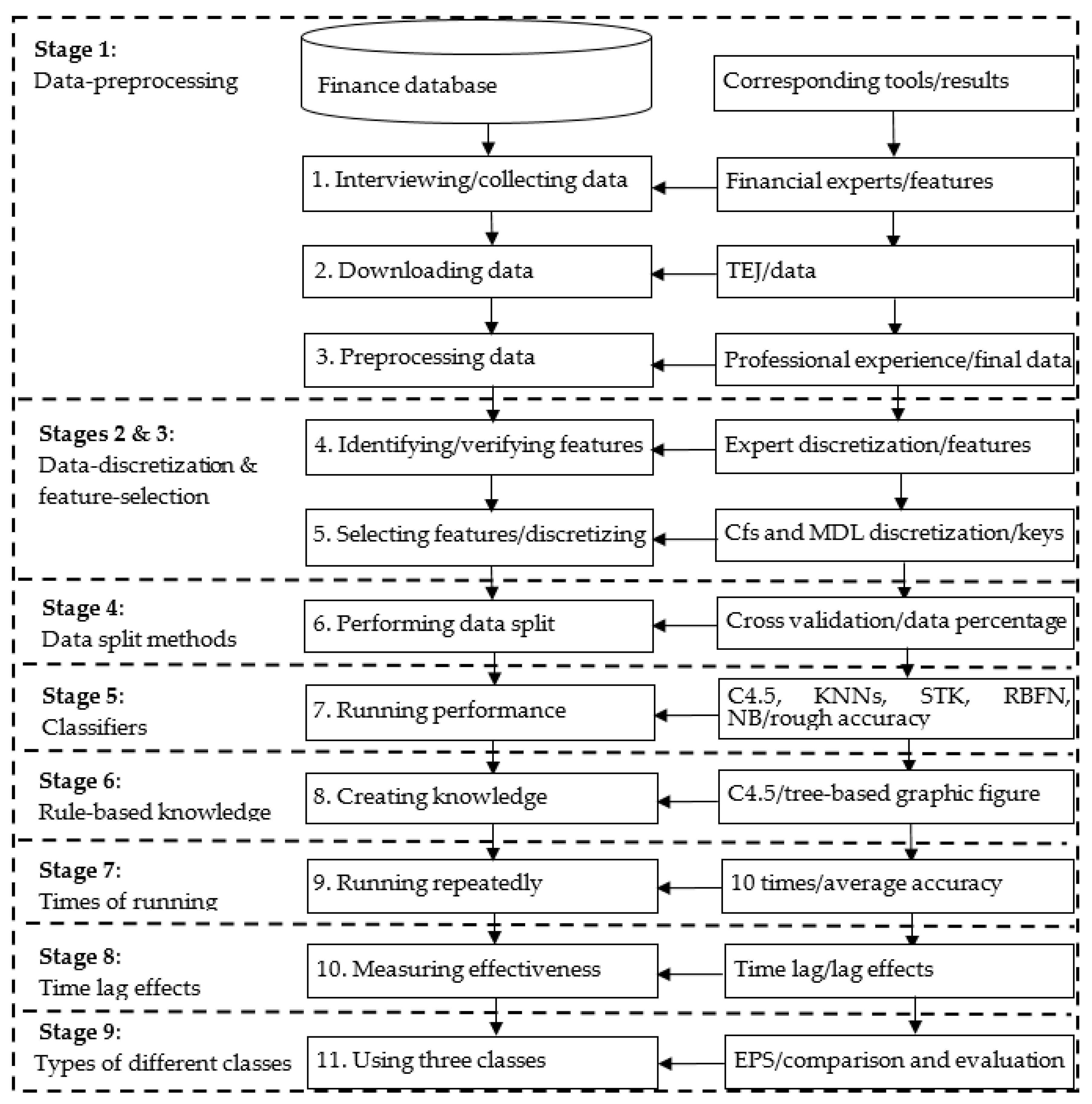
58], they are used as the basis for the complete construction of the study framework. There are nine components (stages), with 11 detailed steps for raising the advantages and rationalities of this study. (1) Data-preprocessing: This component is used to build a tangible benefit from the reviews of literature and experts from a specific database. (2) Data-discretization: The discretization facilitates the use of data from the view of natural language and improves classification accuracy. (3) Feature-selection: This core technique is used to lower data dimension and complexity to speed the benefits of operating experiments. (4) Two data-split methods: The different data-split methods are used for comparison of the review of practical datasets in the same environment. (5) Machine learners: Different classifiers are assessed and compared to discover the best suitable tool for EPS financial diagnosis. (6) Rule-based DT knowledge: The decisional rules generated by the DT-C4.5 algorithm are used for constructing the instructions of the “IF…THEN…” form used to help define a better choice to achieve a specific goal. (7) Different times of running experiments: It has the advantage of determining the performance of various classifiers with the same given data. (8) Time lag effects: The lag effects of different time periods are measured to understand whether the financial data consider a substantial time-lag effect demonstrated by the given data as well as to identify the right time lag. (9) Types of different classes: The merit of measuring different classes is used to define the performance difference of various classifiers. Mainly, the nine major stages systematically detail the computing processes to support a further clear definition, which is described in Figure 1, to present a flowchart of the applied hybrid models proposed to represent data relativity, with the corresponding tools and steps for experiencing the empirical outcomes (results) of EPS.
These abovementioned components are selected based on the following three reasons. First, they had a high level of evaluation in past studies. Second, no one has tried to use them in predicting EPS of financial fields and then created rule-based decisional knowledge for the stock market to address this practical problem. Third, it is worthwhile to explore the interesting issue of multicomponential discretization models, and its application areas of research and its application advantage are accordingly expected and studied here.
From the restricted review, the study has a valuable contribution and directions in which the multicomponential discretization models are very limited and rarely seen for such an industry setting. Thus, the applied hybrid models proposed are of interest, with the uses of the above nine stages with 11 detailed steps. The proposed hybrid models are implemented and executed in a step-by-step mode; some steps (e.g., five classifiers: DT-C4.5, KNNs, STK, RBFN, and NB) are respectively run for each model from a software package tool, and some other steps are coded or stored in the CSV format of Excel software (e.g., data-preprocessing is implemented in Microsoft Excel).

3.2. Algorithm of the Applied Hybrid Models Proposed

In the subsection, this study applies five main hybrid classification models, with nine stages, to address financial application issues related to EPS to find a meaningful empirical research method. To improve the readability of this study, the concepts and structures of these models are addressed in a tableau list report. The main stages of these proposed hybrid models (referred to as Models A–E) are data-preprocessing, data-discretization, feature-selection, data split methods, various classifiers, time-lag effects, and the measurement of two types of classes. Table 1 lists their information in detail below. Interestingly, the order performance for executing data-discretization and feature-selection is evaluated in this study.
The algorithm for the above five hybrid models, with the experience of an empirical case study application extracted from a real financial database in Taiwan, is detailed and implemented in 11 steps systematically, as follows.
Stage 1. Data-preprocessing: Table 1 shows that this component is used in all the applied hybrid models proposed, Models A–E.
Step 1. Consulting field experts and gathering data: In this step, we first interviewed field experts interested in financial analysis and investment management and studied the online financial database of the noted Taiwan Economic Journal (TEJ) [59], which is targeted as the object of the experiments in order to identify and confirm essential features. The 25 essential features, including 24 condition features encoded as X1–X24 and one decision feature (X25) encoded as Class, were first defined with the help of financial experts and literature reviews. Financial experts added the first four extra features (X1–X4; Year, Season, Industrial Classification, and Total Capital) to the list of the 20 features (renamed, in order, as X5–X24) that were seen in Section 2.1. The classes of EPS were suggested by experts.
Step 2. Downloading the data used from the TEJ database: Accordingly, raw data for these features were downloaded as an experimental dataset, with 4702 instances from the TEJ database for a six-year period. For ease of presentation, the dataset is named the TEJ dataset.
Step 3. Preprocessing the data: In further analysis, this step filtered six industries. The six industries are electrical machinery, biotechnology and medical, semiconductor, optoelectronics, electronic components, and shipping industries, which are well-known and of high trading volume among Taiwanese investors. As this was the first attempt to find rules in the Taiwanese stock market, the study chose these industries to begin. To facilitate the operation of the experiment, this step cleared irrelevant columns with incomplete or inaccurate data, added and computed some new columns that were not present in the TEJ dataset (such as times interest earned), joined columns of special stock and common stock as the feature of total capital, reconfirmed the information of the TEJ dataset with official reports reviewed from TWSE, and stored the dataset in Excel software format. Table 2 lists all the feature information with descriptive statistics from the TEJ dataset.
Stages 2 and 3. Data-discretization and feature-selection: Table 1 makes it is clear that the component of data-discretization is only used in Models B, D, and E, and the component of feature-selection is for Models C–E.
Step 4. Identifying and verifying and discretizing features: The decisional feature of this study is defined as EPS, which is divided into two types of two and three classes, and the conditional features are 20 financial ratios plus the related four financial variables of Year, Season, Industrial Classification, and Total Capital, which are listed in Table 2. In two classes, the decisional feature of EPS named as Class is firstly classified into P (>0 in NTD, i.e., positive profit) and N (≦0, negative profit), according to the opinion and selection of three experts.
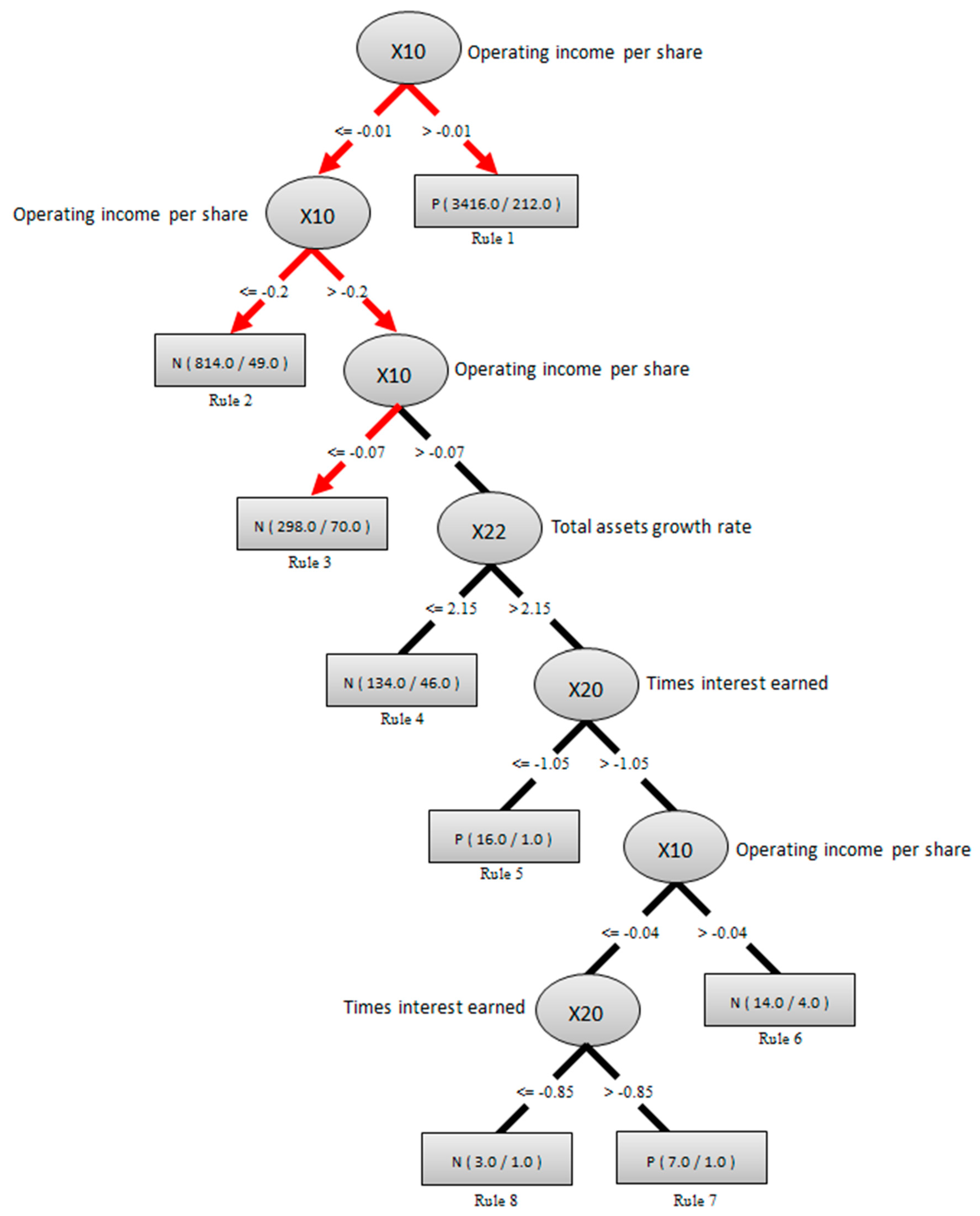
Step 5. Selecting the features and/or discretizing the data: Subsequently, test five organized ways of data-mining the models using various components of data-preprocessing, data-discretization, and feature-selection for performance comparison, including (1) with data-preprocessing but without data-discretization and feature-selection, (2) with data-preprocessing and data-discretization but without feature-selection, (3) with data-preprocessing and feature-selection but without data-discretization, (4) conducting data-preprocessing and data-discretization before feature-selection, and (5) conducting data-preprocessing and feature-selection before data-discretization. The above five ways are mainly measured for component performances by using a Cfs subset evaluation algorithm of search method for feature-selection and a filter function of discretizing tool with minimum description length (MDL) of automatic data-discretization in professional software for data mining techniques from software-defined networks, followed by different classifiers that are executed by employing professional package services. As a result, there are a total of three core determinators, including times interest earned, operating income per share, and total assets growth rate, that are identified in the feature-selection processes for influencing EPS in the type of two classes, which is significantly improved and associated with the stock price of a specific listed stock.
Stage 4. Data-split methods: This component is used for Models A–E.
Step 6. Performing cross-validation and percentage data-split: Furthermore, it is interesting to find out an appropriate model to overcome problems faced in real life by assessing the function of various components of models and then selecting a suitable model. It is desirable to avoid spending a long-time on training a model that is poor. Thus, this step uses two model-selection methods, cross-validation and percentage data-split, when training/testing the processing of the target dataset to make the right selection. On the one hand, based on a study by Džeroski and Zenko [60], the cross-validation method, a general approach for model-selection, is allocated and synthesized with “testing the models with the entire training dataset, and choosing the one that works best” when various models are used with a large set of real problems. In the reviews of model-selection, a basic form of cross-validation divides the dataset into two sets, with the bigger set used for training and the other smaller set used for testing if data are not scarce and are substantial enough to enable input–output measurements. On the contrary, another model-selection approach is to use percentage-split data; it is a popular approach in ML application algorithms from numerous studies [61,62]. The percentage-split for the dataset partitions the original set into different groups of training/testing sub-datasets, such as 90%/10% and 80%/20%. In practice, the training/testing sub-dataset is usually at a 2/1 ratio to achieve a good and reasonable result. To reverify their selection performance, the above two methods are adopted into all the proposed hybrid models, and, from past successful examples, the 10-fold cross-validation and 67%/33% percentage-split of data are commonly used in this step.
Stage 5. Classifiers: This component is used in Models A–E.
Step 7. Applying classifiers and making performance comparisons: Accordingly, run five classifiers (DT-C4.5, KNNs, STK, RBFN, and NB) for each model from the software package tool, with no changes predesigned on these learning classifiers; the five classifiers are selected from performance assessments based on their past high satisfactory results, and their classification performance in accuracy rate due to common use under the two classes of EPS is compared to see and judge their differences that may have some implied information for stock investors. The accuracy rate in one run for these classifiers is then achieved.
Stage 6. Rule-based knowledge: This component is used for Models A–E.
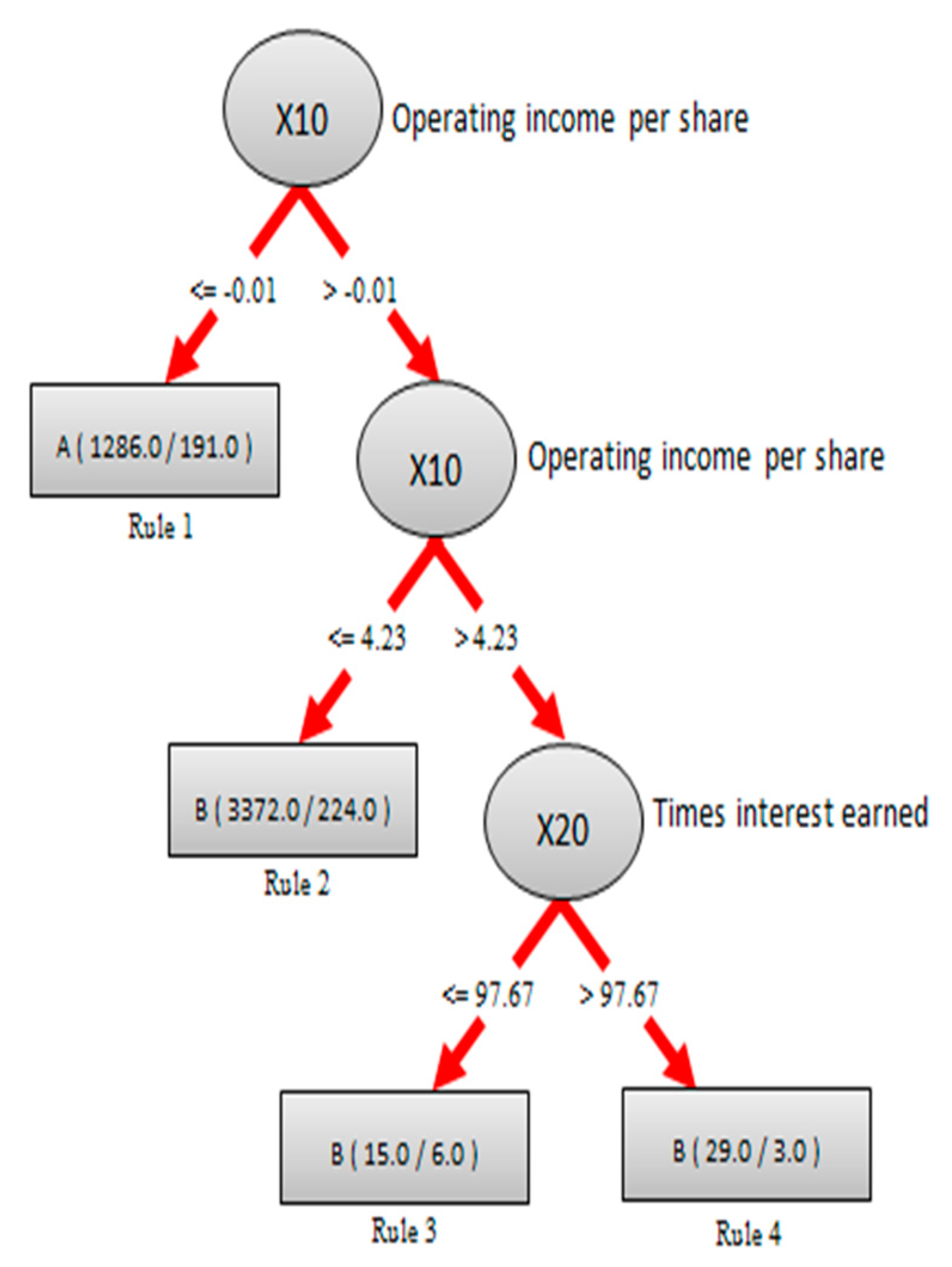
Step 8. Creating rule-based knowledge for interested parties: To generate and understand the hidden information of forming “IF…THEN…” in rule-based knowledge, this step employs a fundamental step of the DT-C4.5 algorithm to create a decisional-tree-based structure (in a graphic figure) to represent the formatted knowledge of the target TEJ dataset. The knowledge in the figure is crucial to a varied topic of EPS in financial investment. For easy presentation and reading, the created tree-based structure (in a graphic figure) and its explanations will be uniformly displayed in the next section.
Stage 7. Times of running experiments: This component is used in Models A–E.
Step 9. Running the experiments repeatedly: To further validate and test the classification accuracy of the five classifiers, the experiment is repeatedly run 10 times for the TEJ dataset, and the average accuracy is obtained for the difference analysis.
Stage 8. Time-lag effects: This component is used for Models A–E.
Step 10. Measuring the effectiveness of time lag: To consider whether time lag has an influence on the prediction of EPS, divide the dataset by seasons, and use the EPS of the current season (T+0), the next season (T+1), the third season (T+2), and the fourth season (T+3) as the decisional feature to test and find the best performing models, which are using the DT-C4.5 and RBFN classifiers and dividing EPS into two classes due to their suitability.
Stage 9. Types of different classes: Finally, this component is used for Models A–E.
Step 11. Using three classes of EPS: To further differentiate and create the class difference, use three classes (i.e., A (<0), B (0~3.75), and C (>3.75)) of EPS based on the automatic discretization recommendation instead of two classes in all the applied hybrid models proposed, and the experiments from Steps 1–10 are run again.

4. Experimental Data Analysis and Research Finding

This section summarizes and concludes the above empirical results in the TEJ dataset on EPS and describes some rule-based knowledge construction, with some followed useful research findings and management implications, and the limitations of the study.

4.1. Empirical Results with Implication

Based on the applied hybrid models proposed with an empirical case study of financial ratios and financial variables, the experimental results are concluded uniformly in some tableau lists for the purposes of performance comparison. Moreover, regarding research-based conclusions, some meaningful information is referenced as a consultant datum to interested parties. First, the performance of models on the tests of cross-validation and percentage-split data was preferentially conducted in view of technical background and support. The cross-validation method selects 90% of the training data subset, and splits 67% of the training data for the other method. Accordingly, the performance of different periods of time-lag effects, different times of running experiments, and different classes were evaluated for the TEJ dataset. Conclusively, the analytical results from all experiments are respectively defined as the following three key points. First, Table 3, Table 4, Table 5 and Table 6 show that the outputs of Steps 1–8 and 11 (i.e., Stages 1–6 and 9) in one run for two data-split methods and two types of classes; second, Table 7, Table 8, Table 9 and Table 10 show the outputs of Steps 1–9 and 11 (i.e., Stages 1–7 and 9) in 10 runs; and third, Table 11, Table 12, Table 13 and Table 14 show the outputs of Steps 1–8 and 10 (i.e., Stages 1–6 and 8) for measuring the time-lag effects.
A total of 10 directions are simply defined from all the main empirical results of the above Table 3, Table 4, Table 5 and Table 6 for Models A–E in the TEJ dataset; they are described as follows.
(1) Performance comparison of models and classifiers: As indicated in the above four tables, seven key results have been determined in terms of models and classifiers, and the shading highlights their significance in the accuracy rate. (a) The poorest accuracy is 75.59%: On average accuracy, Model A has the poorest performance, implying feature-selection and data-discretization could effectively and significantly enhance classification performance. (b) The highest accuracy is 88.14%: On average accuracy, Models D and E have the highest performance, providing valid proof that both feature-selection and data-discretization can improve classification accuracy. (c) The better performance: On total average accuracy, Model B (86.13%) outperforms Model C (81.13%), implying that by comparing the effects of feature-selection with data-discretization, the latter (data-discretization) has more impact on classification performance than on the former feature-selection method. (d) The same accuracy: Models D (87.50%) and E (87.50%) have the same performance in total average accuracy, implying that the executing sequence of feature-selection with data-discretization does not affect model performance. (e) The better average accuracy: Among the five classifiers, DT-C4.5 (91.47%) and RBFN (87.46%) algorithms have better performance than the others in terms of accuracy rate or average accuracy. (f) The best model: Conclusively, Models D and E are the best models both in terms of average accuracy (87.51%) and total average accuracy (87.50%). (g) The best classifier: Conclusively, the DT-C4.5 algorithm wins as the best classifier in terms of both average accuracy (91.49%) and total average accuracy (91.47%).
(2) Assessment of data-discretization: When comparing Model A with Model B in Table 3, Table 4, Table 5 and Table 6, it is clear that Model B has mostly better accuracy than Model A. This information implies that the data-discretization method is an effective tool to improve classification accuracy.
(3) Assessment of feature-selection: Similarly, when comparing Model A with Model C in the same tables, they show that Model C has better accuracy than Model A. This case implies that the feature-selection method benefits classification accuracy.
(4) Measurement of two data-split methods: The analytical results indicate that the cross-validation data approach has higher classification performance than the percentage-split data method in the TEJ dataset when Table 3 and Table 4 are compared with Table 5 and Table 6, respectively.
(5) Measurement of two types of classes of EPS: It is seen that dividing EPS into two classes yields better performance than dividing EPS into three classes. This phenomenon implies a converse management implication that the more classes a decision feature has, the less accuracy the classifier has.
(6) Measurement of two types of running times for experiments: Furthermore, to better justify these comparative results and conclusions, the study repeated the experiments 10 times to compute the mean as well as its standard deviation (S.D.) of the accuracy rate of each setting. Table 7, Table 8, Table 9 and Table 10 show that there are five important viewpoints determined from the views of the mean and standard deviation of accuracy rate for the two data split methods and the two types of classes. (a) As the standard deviations (e.g., 1.00%) of accuracy rates are quite small compared to the mean values (e.g., 87.53%), it is known that the accuracy rates are densely distributed around the mean values. Therefore, the aforementioned conclusions based on the comparisons of average accuracy rates of each model setting are credible. (b) Regarding average accuracy, Models D and E have the same performance (i.e., 87.53%, 87.46%, 87.09%, and 87.04%) and win this accuracy competition regardless of two or three classes in 10 runs. (c) As for the standard deviation of average accuracy, Models D and E have a lower value (e.g., 1.00% < 1.07% < 1.58% < 1.61%, from Table 7) of relative stability, and it implies that the data-discretization and feature-selection methods not only improve classification accuracy but also enhance their high stability regardless of two or three classes in 10 runs. (d) It was found that the percentage-split data method in Models A (e.g., 75.69% > 75.52%) and B (e.g., 86.39% > 86.24%) has a better performance than the cross-validation method regardless of two and three classes. Conversely, the percentage-split data method in Models C–E (e.g., 78.19% < 78.31% and 87.46% < 87.53%) has less performance than the cross-validation method regardless of two and three classes. This interesting problematic issue should be further explored and examined in subsequent research. (e) More interestingly, the accuracy of 91.43% of DT-C4.5 in Model A without exogenous data-discretization and feature-selection has the second-highest accuracy in the 10 runs. A rational basis about the special case is that the DT-C4.5 algorithm already has an endogenous function of data-discretization and feature-selection, which is more suitable for the TEJ dataset than other methods.
(7) Measurement of time-lag effects: To test the influence that time lag has on EPS, the study ran the first two better-performing models found by using the classifiers of DT-C4.5 and RBFN in two classes. Table 11, Table 12, Table 13 and Table 14 mainly show that there are four key directions useful to understanding the time effectiveness of rule-making for investors. (a) It is implied that the less the time lag, the higher the accuracy, and vice versa, regardless of data cross-validation or percentage-split methods and two or three classes. This analytical result indicates and implies that the models could not predict EPS in the far future and support the treatment of using the current season’s EPS in most of the TEJ dataset. (b) Most of the rank of performance is followed by (T+0) ➔ (T+1) ➔ (T+2) ➔ (T+3) (e.g., 91.43% > 83.25% > 78.89% > 76.79% in Model A from Table 11), which shows in the cross-validation method in two classes for RBFN classifier. (c) From Model A, when Table 11 and Table 12 are compared to Table 13 and Table 14, it clearly indicates that DT-C4.5 (e.g., (91.38% and 92.06%) > (86.58% and 87.55%)) significantly outperforms RBFN in average accuracy, and it was found that the RBFN algorithm needs the support of some external techniques like feature-selection and data-discretization methods to improve its classification accuracy. (d) The above information implies that some classifiers in stand-alone models require some special methods to support its classification ability, and it implies hybrid models perform better than stand-alone models.
(8) Results of data-discretization: According to the estimation from Model E in two classes, Table 15 lists the results of the data-discretization method after implementing feature-selection. Table 15 shows that the three key condition features, X10, X20, and X22, are discretized into six, six, and five intervals based on the automatic discretization method, which correspond to linguistic terms A_1–A_6, B_1–B_6, and C_1–C_5, respectively. The decisional feature is discretized into two intervals (i.e., P and N), as suggested by three financial experts. These linguistic terms are referred to as a natural language, which is useful and helpful to good understanding and decision-making. For example, the linguistic terms A_1–A_6 are referenced as very low, low, medium, medium–high, high, and very high, respectively. Moreover, the data-discretization method for setting the linguistic terms improves the classification accuracy.
(9) Results of feature-selection: According to the estimation from Steps 4 and 5, three important factors, including total assets growth rate, times interest earned, and operating income per share, are specified in the feature-selection method for the two classes of EPS; simultaneously, two key features, times interest earned and operating income per share, are defined for the three classes. Obviously, the two key factors of times interest earned and operating income per share are identified in both the two and three classes.
(10) Additional measurement of hybrid models with stand-alone models: To further evaluate the capacity between the applied hybrid models proposed and the stand-alone models [18,30,34,45,54], the stand-alone models were run and their classification accuracy was achieved, respectively, in the two and three classes. Subsequently, the applied hybrid models proposed had the best of 92.46% compared to that of each stand-alone model, regardless of two or three classes. Clearly, the hybrid models did better than the stand-alone models used for the empirical case of this study.

4.2. Rule-based Knowledge Construction

The decision-rule-based trees created by the C4.5 algorithm in Step 8 of the applied hybrid models proposed, as well as three key features for influencing EPS, including times interest earned, total assets growth rate, and operating income per share, were determined. Figure 2 and Figure 3 depict the framework of the tree-based rules in an interactive visualization form below. To illustrate the forming processes of the rules effectively, examples of some rules (highlighted in red in the type of two classes and three classes) are indicated in EPS object-oriented interpretations for explaining financial ratios and variables applications using advanced multicomponential discretization models toward a solution of big data benchmarks.
For example, the explanation of three rules in Figure 2 is described in detail, as follows:
(1) Rule 1: => IF X10 > −0.01 THEN Class = P.
This information of rule indicates that if only the feature of operating income per share (i.e., X10) is more than -0.01 (in NT$), then the EPS of a listed specific stock (i.e., a specific company) will be a positive profit. Thus, this study infers and forecasts that this listed stock will have an uptrend price associated with Rule 1 in the future.
(2) Rule 2: => IF X10 ≦ −0.01 and X10 ≦ −0.20 THEN Class = N.
This information of rule indicates that if the feature of operating income per share is less than or equal to -0.0 and -0.20, then the EPS of a listed specific stock will be a negative profit. Similarly, this study infers and forecasts that this listed stock will have a downtrend price associated with Rule 2 in the future.
(3) Rule 3: => IF X10 ≦ −0.01 and X10 > −0.20 and X10 ≦ −0.07 THEN Class = N.
This information of the rule indicates that if the feature of operating income per share is less than or equal to −0.01 and more than −0.20 and less than or equal to −0.07, then the EPS of a listed specific stock will be a negative profit. Additionally, this study infers and forecasts that this listed stock will have a downtrend price associated with Rule 3 in the future.
Certainly, following the same method, Rules 4–8 in Figure 2 are also formatted in the form “IF… THEN…” of rule-based knowledge construction.
Furthermore, their explanation for the four rules in Figure 3 is described, as follows:
(1)
Rule 1: => IF X10 ≦ −0.01 THEN Class = A, or semantically low EPS.
This rule indicates that if only the feature of operating income per share (i.e., X10) is less than −0.01 (in NTD), then the EPS of a listed specific stock will have nonpositive benefits.
(2)
Rule 2: => IF −0.01 > X10 ≦ 4.23 THEN Class = B, or semantically medium EPS.
This rule indicates that if only the feature of operating income per share is in this range (-0.01 > X10 ≦ 4.23), then the EPS of a listed specific stock will have a result between 0 and 3.75.
(3)
Rule 3: => IF X10 > 4.23 and X20 ≦ 97.67 THEN Class = B, or semantically medium EPS.
This rule indicates that if the feature of operating income per share is greater than 4.23, and times interest earned (i.e., X20) is equal or less than 97.67, then the EPS of a listed specific stock will have a result between 0 and 3.75.
(4)
Rule 4: => IF X10 > 4.23 and X20 > 97.67 THEN Class = C, or semantically high EPS.
This rule indicates that if the feature of operating income per share is greater than 4.23, and times interest earned is greater than 97.67, then the EPS of a listed specific stock will have a result higher than 3.75.
Table 3, Table 4, Table 5 and Table 6 illustrate the rule-based knowledge that could predict EPS with an accuracy rate of above 90%, which is a high accuracy to predict real targets. Following the rules in Figure 2 and Figure 3, investors can easily consider and select positive/negative information of listed stock for their well-maintained investment portfolios with a positive affirmation.

4.3. Helpful Research Findings and Management Implications

To further mine the empirical information hidden in the TEJ dataset, the experimental results yield the following 11 useful research findings.
(1) Benefit of feature-selection: Through the Cfs algorithm for feature-selection in two classes, five features remained and 20 features were removed. In particular, the accuracy of the applied hybrid Models D and E proposed, with the five used features, still had significant performances when compared with the other listed models using the original features under the same settings. Based on Thangavel and Pethalakshmi [63], their postreduction performance of an experiment result showed that the hybrid model using the features after feature-selection had higher classification accuracy than the original features for the same conditions; the experimental results proved that the reasonably practicable solution of feature-selection techniques effectively reduces the features, yielding better accuracy than that of the original feature set.
(2) Feature-selection-based discretization method: After performing the feature-selection function, it was found, interestingly, that some key features were discretized into meaningful linguistic terms (e.g., small, medium, and large) of natural language by data-discretization methods to assist rule-based knowledge construction; concurrently, the functions of combining feature-selection with data-discretization works uncommonly improved classification accuracy.
(3) Important discovery from the functions of feature-selection and data-discretization works: It was found that the execution order for performing the works of feature-selection and data-discretization had clearly indicated no performance difference between the listed two methods of functional components when Table 3, Table 4, Table 5 and Table 6 were compared to Table 7, Table 8, Table 9 and Table 10, respectively.
(4) Interpretation of constructing the decision rule-based knowledge: This study generates some comprehensible decision-rule-based knowledge to explain how to use the graphic-based information visualization created by the C4.5 algorithm for investors to enable knowledge formation.
(5) Selection of good financial status EPS: From Figure 2 and Figure 3, this study discovered important rules for the positive/negative status of listed stock, which can help investors to manage effective investment strategy.
(6) The best practice of enablers: From the study results, it was found that the best classifier is the decision tree C4.5 algorithm for the TEJ dataset, and the best model is Models D and E in terms of average accuracy.
(7) Interpretation of two data-split methods: It was found that the cross-validation data approach makes more appropriate use of the TEJ dataset than the percentage-split data approach.
(8) Interpretation of different running times of experiments: It was found that the rank of average accuracy for the Models D and E ➔ Model B ➔ Model C ➔ Model A is the same between one run and 10 runs of experiments, regardless of different data-split methods and two types of classes of EPS.
(9) Difference interpretation for different types of classes of EPS: It was found that a difference exists within the key features when different types of classes in the same decision feature of EPS are used.
(10) Effects of time lag for the financial industries: From Table 11, Table 12, Table 13 and Table 14, the applied hybrid models proposed have the best classification capacity when the time lag reaches time T+0, and they do not have a deferred effect in the TEJ dataset on some public listed companies of Taiwan’s stock market.
(11) Identification of the two most key determinants: From the above experimental results, two key features, operating income per share and times interest earned, are identified, regardless of two or three classes of EPS.
Three meaningful management implications from the empirical results of this study are found and catalogued.
(1) For individual investors: Three major attributes, total assets growth rate, times interest earned, and operating income per share, have been sorted out and deserve more attention from dozens of financial ratios when conducting fundamental analysis of a listed stock. The construction of knowledge-based decision rules provides effective instructs to select a proper target from the sea of considerable potential stocks.
(2) For investment-technology-developing companies: DT-C4.5 and RBFN are two good targets of classifiers suitable for predicting EPS in the TWSE with some empirical evidence. Investment decision support systems based on data-mining techniques deserve further valuable assessments and developments in the future.
(3) For practitioners and academicians: The experimental results are valuable information helpful to them by closing the knowledge gap between theoretical frameworks and evidence-based practices in future research.

4.4. Closing the Gap Report from the Applied Hybrid Models Proposed

Table 3, Table 4, Table 5, Table 6, Table 7, Table 8, Table 9, Table 10, Table 11, Table 12, Table 13 and Table 14 clearly indicate that this study has four practical values to bridge the gap between past studies and this study, as follows: (1) The practical gap in field applications is filled with a small step for providing applicable remarks and practical experiences to control the performance of profit-making of the associated EPS classification for investors used in the financial environment. (2) The gap of technical services has been closed since the study has made an advanced appropriate hybrid model offered to the stock market application field. (3) The gap of knowledge creation to review applicable decision-rule-based diagnostic systems for identifying EPS has been closed with the successful results in financial ratio verification. (4) Moreover, the study bridges the gap of the lack of literature on EPS application support.

4.5. Research Limitations of the Study

Although the study is empirically valid, the following limitations must be noted and addressed in the future:
(1)
A significant shortfall of this study is that the sample used only listed companies on the TWSE. Investor choice, such as companies traded over the counter and emerging the stock market, was not considered in this study, and there are 969 such companies currently operating, which is quite large.
(2)
Another limitation of this study is that the pool of possible predictors is confined to company financial statements, but, for the work of forecasting EPS, a broader range of information sources may be considered.
(3)
The financial ratios and variables were predefined and calculated from financial statements of online databases, and researchers should have professional knowledge of this industry background and environment to know the financial topics better.
(4)
The classifiers were limited to DT-C4.5, KNNs, STK, RBFN, and NB, which were used and validated. Future studies may take other classification algorithms in hybrid and stand-alone models into account for a generalized application in the identification of EPS for financial diagnosis.

5. Discussion

In the data-mining and machine-learning fields [64,65,66], so many challenges trigger the researchers’ ability. Developing a model to overcome a dilemma in decision-making for financial analysts is necessary. This study proposed an advanced hybrid model [67] to fulfill a valuable research need for classifying EPS with good identification of financial ratios for various categories from large-scale data structures, with the empirical results as desired. However, regarding the key components of the applied hybrid models proposed, it was determined that three directions are required to ascertain the intrinsic needs of the experiences for this study.
First, financial data are continuous and of a big volume. Pal and Kar [68] suggested using the data-discretization technique to improve classification performance. Data-discretization could reduce the number of generated classifying rules, enhance the performance of classifiers, and ease the semantic representation. This study, through model performance comparison and the illustration of decision rule-based knowledge, confirmed Pal and Kar’s study [68].
Second, feature-selection is a suggested technique to tackle big data by reducing the complexity of multifaceted data across disciplines [66,69]. Seeja [70] had mentioned several benefits of performing feature-selection functions, such as simplifying the model or accelerating model building and knowledge forming. The results of model performance comparisons and the generated simple DTs in this study were in line with Seeja’s proposition [70]. This study has tested the effect of a sequence in applying data-discretization and feature-selection and found no difference between them. It was found that feature-selection had less impact on accuracy than data-discretization did. However, this study conjectured that the performance was determined by the fit between model and data because the reported performance from different model settings remained mixed.
Third, the five classifiers tested were all well-known and reported with good performance in previous studies. However, the performance of the learning classifier is strongly limited for some cases applied, such as the dependence of instance complexity [71], the objective of study [72], the subject experience of users [73], and the application field [74]. In particular, Tabassum [71] indicated that the performance of the classifiers was varied among data domains, such as the framework of the number of instances or attributes used in the experiences from the learning classifiers. It is problematic and difficult to mine suitable learning classifiers with the best performance from experimental instances. Interestingly, this study confirmed Tabassum’s study [71]. With reference to the study results, DT-C4.5 and RBFN outperformed other classifiers significantly, indicating that there is no classifier universally good or poor in terms of classification performance. The reason for this is that DT-C4.5 and RBFN performed better than others, which may lie in the inherent nature of the Taiwanese stock market. Therefore, future studies require a greater variety of input data that might further test the proposition of fit between model and data, as well as explore the proper dimensions to describe the implicit nature of data to explain the fit.

6. Conclusions

Classifying EPS with financial ratios and variables has practical and researchable values in financial management and stock investment. This study contributed five hybrid models with advanced multicomponential discretization methods to use different classifiers of ML technologies to find key functions of data-discretization, feature-selection works, two data split methods, rule-based knowledge construction, effects of time lag, different running times of experiments, and two types of different classes in model building. This study also identified that DT-C4.5 and RBFN were relatively efficient classifiers for identifying positive EPS stocks from enormous financial ratio applications in the TEJ dataset for large-scale data analytics and solutions. Simultaneously, total assets growth rate, times interest earned, and operating income per share showed a specific feature-selection advantage in two classes of EPS. Particularly for Table 7, Table 8, Table 9 and Table 10, some core results were concluded. (1) Most of Models D and E had higher accuracy rates with a lower standard deviation for the comparison of average accuracy. (2) Models D and E had the best accuracy and the same performance in average accuracy in 10 runs. (3) Feature-selection and data-discretization techniques had abilities for accuracy improvement and the stability of model implementation in the TEJ dataset. (4) Regarding the percentage-split data method, Models A and B had better performance than the cross-validation method; however, Models C–E for the percentage-split data method had worse performance than the cross-validation method. (5) Better accuracy, 91.43%, for DT-C4.5 in Model A was better suited than other classifiers for the cross-validation method. As for the better classification accuracy from all the experiments in Table 3, Table 4, Table 5, Table 6, Table 7, Table 8, Table 9, Table 10, Table 11, Table 12, Table 13 and Table 14, four empirical results were identified for the TEJ dataset. (1) The highest accuracy of 92.46% occurred in Model C, using decision tree learning with the percentage-split method in two classes for one run. (2) The mean of highest accuracy, 91.44%, occurred in Models D and E using naïve Bayes learning, both with the cross-validation method and the percentage-split method in two classes for 10 runs. (3) The mean of highest average accuracy, 87.53%, occurred in Models D and E with the cross-validation method in two classes. (4) The highest accuracy of 92.46% occurred in Model C using decision tree learning-C4.5 with the percentage-split method and no time lag in two classes. It is feasible, due to the methodology used in this study, that the classifiers learned an acceptable classification accuracy rate and achieved an adequate ranking in the related financial characteristics applied. The proposed method provided a better possible way for a ranking, mentioned above, of the learning classifiers.
Stock selection is a real-world problem with a trade-off between risk and profit because returns from stock investments are risky. This study provides an alternate model to identify a good EPS stock associated with an expected high stock price, with risk aversion adequately and effectively addressed. Hence, in terms of research contribution, this study concludes that various performance measurements of multicomponents for comparison intentions, when searching for a suitable means and tool, are useful for financial analysts. Empirically, the analytical results showed that data-discretization and feature-selection with some classifiers had significantly better accuracy with a satisfactory result. There are five key findings identified and concluded from the empirical results. (1) Model A is the poorest one as it is without the key techniques of data-discretization and feature-selection; the abovementioned information implies that the hybrid models have better performance than that of stand-alone models. (2) Regarding model components used in this study, their performance degree is further assessed under various evaluation criteria for universal application in subsequent research. (3) From Pal and Kar [68], it was found that data first need to be discretized when putting it into a classification model. Thus, the MDL of automatic data-discretization to build thresholds in increasing performance provides just such a prominent example with good satisfaction to validate the importance of using rule-based models in this study. The above-detailed knowledge intensifies the requirement of discretizing data of the conditional features for financial applications. (4) The study results on data-discretization performance are matched and affirmed with the literature [68]. (5) Furthermore, the key data-discretization methods have been used as a useful tool for defining purposeful linguistic terms in natural language for manipulating rule-based knowledge representation. This study conclusively makes a valuable contribution to useful research findings, managerial implications, and technical directions in which multicomponential discretization models are limited and rarely seen for such an industry setting, from the restricted reviews. This study is a stepping stone on the road towards an advanced data-mining application for financial data resolution [75,76], with some meaningful differentiation from past studies and having sentimental value. Furthermore, this study’s originality is in the devising of multimodels with advanced settings to identify the best model and set for anticipating the EPS of Taiwanese companies.
In future studies, there is a need for expansion defined as follows: (1) For example, use the applied hybrid models proposed to analyze datasets from different industries and measure the model-selection performance. (2) It helps address good concerns to validate the same financial datasets, but collected from other countries, to develop different hybrid models, to use different years of financial datasets, and to evaluate the performance difference. (3) Future studies may take a variety of various companies into account for a well-identified application. Thus, other companies from different industries other than those used in this study may be studied for comparison. (4) In addition, different characteristics of features, such as market efficiency, might influence the model-selection of predictors or classifiers, which should be considered in the future. (5) Different discretization data techniques in identifying the EPS feature are worthy of future consideration in the applied hybrid models proposed; likewise, different feature-selection methods should be explored for the same purposes. (6) Various types of decisional features other than two and three classes of financial EPS status are necessary to retest the function of the hybrid models. (7) Extra conditional features differentiated from the study should be measured with the hybrid models. (8) Different time-lag effects should be further identified for measuring later events on the basis of the former ones in order to further validate the application function of the hybrid models. (9) In particular, the plan to add geo-information of firm locations to the TEJ dataset in Taiwan and to test a wider variety of classifiers to compare their performances is an interesting issue since stocks are a famous investment portfolio for global world investors. Taiwan is located over the Taiwan Strait, away from mainland China, with a 180-km distance. Regarding the stock market of mainland China, the three interests of Hong Kong Exchanges and Clearing Limited (HKEx), Shenzhen Stock Exchange (SZSE), and Shanghai Stock Exchange (SSE) are major stock markets with distinct characteristics from TWSE. Many geographically related interesting financial facts and rules about the companies reside in the big data of the four stock markets. Subsequent studies may research the EPS of companies in SSE, SZSE, and HKEx to construct a map of the Chinese stock market with rich features. (10) Exploring the topic is concerned with how these proposed hybrid models increase financial EPS to provide further verification. Additionally, differentiating and learning the function before/after feature-selection and data-discretization techniques in the study is needed in subsequent research.

Author Contributions

Conceptualization, H.-C.H.; methodology, H.-C.H. and Y.-S.C.; software, S.-F.C.; validation, Y.-S.C. and S.-F.C.; formal analysis, S.-F.C.; investigation, Y.-S.C. and A.K.S.; resources, Y.-S.C.; data curation, S.-F.C.; writing—original draft preparation, H.-C.H.; writing—review and editing, Y.-S.C. and A.K.S.; visualization, Y.-S.C. and A.K.S. All authors have read and agreed to the published version of the manuscript.

Funding

This research was funded by the Ministry of Science and Technology of Republic of China, Taiwan, grant number MOST 108-2410-H-146-001.

Acknowledgments

The authors would like to cordially express many thanks for the above financial support of this paper. The authors also sincerely appreciate the editors and the four anonymous referees for their constructive comments and helpful suggestions to improve the quality of the paper.

Conflicts of Interest

The authors declare no conflict of interest.

References

  1. Allen, K.D.; Winters, D.B. Auditor response to changing risk: Money market funds during the financial crisis. Rev. Quant. Financ. Account. 2020. [Google Scholar] [CrossRef]
  2. Cai, S.; Zhang, J. Exploration of credit risk of P2P platform based on data mining technology. J. Comput. Appl. Math. 2020, 372, 112718. [Google Scholar] [CrossRef]
  3. Wang, Z.; Yin, J. Risk assessment of inland waterborne transportation using data mining. Marit. Policy Manag. 2020, 47, 633–648. [Google Scholar] [CrossRef]
  4. Wang, G.; Miao, J. Design of data mining algorithm based on rough entropy for US stock market abnormality. J. Intell. Fuzzy Syst. 2020, 1–9. [Google Scholar] [CrossRef]
  5. Dimitrakopoulos, S.; Kolossiatis, M. Bayesian analysis of moving average stochastic volatility models: Modeling in-mean effects and leverage for financial time series. Econ. Rev. 2020, 39, 319–343. [Google Scholar] [CrossRef]
  6. Muruganandan, S. Testing the profitability of technical trading rules across market cycles: Evidence from India. Colombo Bus. J. 2020, 11, 24–46. [Google Scholar] [CrossRef]
  7. Hung, N.H. Various moving average convergence divergence trading strategies: A comparison. Invest. Manag. Financ. Innov. 2016, 13, 1–7. [Google Scholar] [CrossRef]
  8. Chahine, S.; Malhotra, N.K. Impact of social media strategies on stock price: The case of Twitter. Eur. J. Mark. 2018, 52, 1526–1549. [Google Scholar] [CrossRef]
  9. Cuestas, J.C.; Huang, Y.S.; Tang, B. Does internationalisation increase exchange rate exposure?—Evidence from Chinese financial firms. Int. Rev. Financ. Anal. 2018, 56, 253–263. [Google Scholar] [CrossRef]
  10. Mehlawat, M.K.; Kumar, A.; Yadav, S.; Chen, W. Data envelopment analysis based fuzzy multi-objective portfolio selection model involving higher moments. Inf. Sci. 2018, 460–461, 128–150. [Google Scholar] [CrossRef]
  11. Choi, H.; Son, H.; Kim, C. Predicting financial distress of contractors in the construction industry using ensemble learning. Expert Syst. Appl. 2018, 110, 1–10. [Google Scholar] [CrossRef]
  12. Lu, R.; Wei, Y.C.; Chang, T.Y. The effects and applicability of financial media reports on corporation default ratings. Int. Rev. Econ. Financ. 2015, 36, 69–87. [Google Scholar] [CrossRef]
  13. Kadim, A.; Sunardi, N.; Husain, T. The modeling firm’s value based on financial ratios, intellectual capital and dividend policy. Accounting 2020, 6, 859–870. [Google Scholar] [CrossRef]
  14. Bagina, R.W. Assessing the financial statement (ratios) of Anglogold-Ashanti Limited, Ghana. Asian J. Econ. Bus. Account. 2020, 14, 45–55. [Google Scholar] [CrossRef] [Green Version]
  15. Sriram, M. Do firm specific characteristics and industry classification corroborate voluntary disclosure of financial ratios: An empirical investigation of S&P CNX 500 companies. J. Manag. Gov. 2020, 24, 431–448. [Google Scholar] [CrossRef]
  16. Cengiz, H. The relationship between stock returns and financial ratios in Borsa Istanbul analysed by the classification tree method. Int. J. Bus. Emerg. Markets 2020, 12, 204–216. [Google Scholar] [CrossRef]
  17. Mita, A.F.; Utama, S.; Fitriany, F.; Wulandari, E.R. The adoption of IFRS, comparability of financial statements and foreign investors’ ownership. Asian Rev. Account. 2018, 26, 391–411. [Google Scholar] [CrossRef]
  18. Rawal, B.; Agarwal, R. Improving accuracy of classification based on C4.5 decision tree algorithm using big data analytics. Adv. Intell. Syst. Comput. 2019, 711, 203–211. [Google Scholar]
  19. Lee, C.-T.; Horng, S.-C. Abnormality detection of Cast-Resin transformers using the fuzzy logic clustering decision tree. Energies 2020, 13, 2546. [Google Scholar] [CrossRef]
  20. Ghasemi, E.; Gholizadeh, H.; Adoko, A.C. Evaluation of rockburst occurrence and intensity in underground structures using decision tree approach. Eng. Comput. 2020, 36, 213–225. [Google Scholar] [CrossRef]
  21. Saadatfar, H.; Khosravi, S.; Joloudari, J.H.; Mosavi, A.; Shamshirband, S. A new K-nearest neighbors classifier for big data based on efficient data pruning. Mathematics 2020, 8, 286. [Google Scholar] [CrossRef] [Green Version]
  22. Gohari, M.; Eydi, A.M. Modelling of shaft unbalance: Modelling a multi discs rotor using K-Nearest Neighbor and Decision Tree Algorithms. Measurement 2020, 151, 107253. [Google Scholar] [CrossRef]
  23. Qaddoura, R.; Faris, H.; Aljarah, I. An efficient clustering algorithm based on the k-nearest neighbors with an indexing ratio. Int. J. Mach. Learn. Cybern. 2020, 11, 675–714. [Google Scholar] [CrossRef]
  24. Tran, H.Q.; Ha, C. High precision weighted optimum K-Nearest Neighbors algorithm for indoor visible light positioning applications. IEEE Access 2020, 8, 114597–114607. [Google Scholar] [CrossRef]
  25. Tjahjadi, H.; Ramli, K. Noninvasive blood pressure classification based on Photoplethysmography using K-Nearest Neighbors algorithm: A feasibility study. Information 2020, 11, 93. [Google Scholar] [CrossRef] [Green Version]
  26. Fiorentini, N.; Losa, M. Handling imbalanced data in road crash severity prediction by machine learning algorithms. Infrastructures 2020, 5, 61. [Google Scholar] [CrossRef]
  27. Cai, W.; Pan, W.; Liu, J.; Chen, Z.; Ming, Z. k-Reciprocal nearest neighbors algorithm for one-class collaborative filtering. Neurocomputing 2020, 381, 207–216. [Google Scholar] [CrossRef]
  28. Ala’raj, M.; Majdalawieh, M.; Abbod, M.F. Improving binary classification using filtering based on k-NN proximity graphs. J. Big Data 2020, 7, 15. [Google Scholar] [CrossRef]
  29. Zhang, X.; Han, N.; Qiao, S.; Zhang, Y.; Huang, P.; Peng, J.; Zhou, K.; Yuan, C.-A. Balancing large margin nearest neighbours for imbalanced data. J. Eng. 2020, 2020, 316–321. [Google Scholar] [CrossRef]
  30. Prajapati, B.P.; Kathiriya, D.R. A hybrid machine learning technique for fusing fast k-NN and training set reduction: Combining both improves the effectiveness of classification. Adv. Intell. Syst. Comput. 2019, 714, 229–240. [Google Scholar]
  31. Jiang, M.; Liu, J.; Zhang, L.; Liu, C. An improved Stacking framework for stock index prediction by leveraging tree-based ensemble models and deep learning algorithms. Phys. A Stat. Mech. Appl. 2020, 541, 122272. [Google Scholar] [CrossRef]
  32. Pisula, T. An ensemble classifier-based scoring model for predicting bankruptcy of polish companies in the Podkarpackie Voivodeship. J. Risk Financ. Manag. 2020, 13, 37. [Google Scholar] [CrossRef] [Green Version]
  33. Soui, M.; Smiti, S.; Mkaouer, M.W.; Ejbali, R. Bankruptcy prediction using stacked auto-encoders. Appl. Artif. Intell. 2020, 34, 80–100. [Google Scholar] [CrossRef]
  34. García, V.; Marqués, A.I.; Sánchez, J.S. Exploring the synergetic effects of sample types on the performance of ensembles for credit risk and corporate bankruptcy prediction. Inf. Fusion 2019, 47, 88–101. [Google Scholar] [CrossRef]
  35. Liang, D.; Tsai, C.F.; Lu, H.Y.R.; Chang, L.S. Combining corporate governance indicators with stacking ensembles for financial distress prediction. J. Bus. Res. 2020, 120, 137–146. [Google Scholar] [CrossRef]
  36. Khan, W.; Ghazanfar, M.A.; Azam, M.A.; Karami, A.; Alyoubi, K.H.; Alfakeeh, A.S. Stock market prediction using machine learning classifiers and social media, news. J. Ambient Intell. Hum. Comput. 2020. [Google Scholar] [CrossRef]
  37. Saha, M.; Santara, A.; Mitra, P.; Chakraborty, A.; Nanjundiah, R.S. Prediction of the Indian summer monsoon using a stacked autoencoder and ensemble regression model. Int. J. Forecast. 2020. [Google Scholar] [CrossRef]
  38. Patil, P.R.; Sivagami, M. Forest cover classification using stacking of ensemble learning and neural networks. In Artificial Intelligence and Evolutionary Computations in Engineering Systems. Advances in Intelligent Systems and Computing; Dash, S., Lakshmi, C., Das, S., Panigrahi, B., Eds.; Springer: Singapore, 2020; Volume 1056, pp. 89–102. [Google Scholar]
  39. Zheng, S.; Zhao, J. A new unsupervised data mining method based on the stacked autoencoder for chemical process fault diagnosis. Comput. Chem. Eng. 2020, 135, 106755. [Google Scholar] [CrossRef]
  40. Liu, H.; Long, Z. An improved deep learning model for predicting stock market price time series. Digital Signal Process. 2020, 102, 102741. [Google Scholar] [CrossRef]
  41. Ribeiro, M.H.D.M.; dos Santos Coelho, L. Ensemble approach based on bagging, boosting and stacking for short-term prediction in agribusiness time series. Appl. Soft Comput. 2020, 86, 105837. [Google Scholar] [CrossRef]
  42. Kanazawa, N. Radial basis functions neural networks for nonlinear time series analysis and time-varying effects of supply shocks. J. Macroecon. 2020, 64, 103210. [Google Scholar] [CrossRef]
  43. Mansor, M.A.; Mohd Jamaludin, S.Z.; Mohd Kasihmuddin, M.S.; Alzaeemi, S.A.; Md Basir, M.F.; Sathasivam, S. Systematic boolean satisfiability programming in radial basis function neural network. Processes 2020, 8, 214. [Google Scholar] [CrossRef] [Green Version]
  44. Teixeira Zavadzki de Pauli, S.; Kleina, M.; Bonat, W.H. Comparing artificial neural network architectures for Brazilian stock market prediction. Ann. Data Sci. 2020. [Google Scholar] [CrossRef]
  45. Mirjalili, S. Evolutionary radial basis function networks. Stud. Comput. Intell. 2019, 780, 105–139. [Google Scholar]
  46. Buhmann, M.; Jäger, J. Multiply monotone functions for radial basis function interpolation: Extensions and new kernels. J. Approx. Theory 2020, 256, 105434. [Google Scholar] [CrossRef]
  47. Karimi, N.; Kazem, S.; Ahmadian, D.; Adibi, H.; Ballestra, L.V. On a generalized Gaussian radial basis function: Analysis and applications. Eng. Anal. Bound. Elem. 2020, 112, 46–57. [Google Scholar] [CrossRef]
  48. Soradi-Zeid, S. Efficient radial basis functions approaches for solving a class of fractional optimal control problems. Comput. Appl. Math. 2020, 39, 20. [Google Scholar] [CrossRef]
  49. Nabipour, M.; Nayyeri, P.; Jabani, H.; Shahab, S.; Mosavi, A. Predicting stock market trends using machine learning and deep learning algorithms via continuous and binary data: A comparative analysis. IEEE Access 2020, 8, 150199–150212. [Google Scholar] [CrossRef]
  50. Vismayaa, V.; Pooja, K.R.; Alekhya, A.; Malavika, C.N.; Nair, B.B.; Kumar, P.N. Classifier based stock trading recommender systems for Indian stocks: An empirical evaluation. Comput. Econ. 2020, 55, 901–923. [Google Scholar] [CrossRef]
  51. Bhandare, Y.; Bharsawade, S.; Nayyar, D.; Phadtare, O.; Gore, D. SMART: Stock Market Analyst Rating Technique Using Naive Bayes Classifier. In Proceedings of the 2020 International Conference for Emerging Technology (INCET), Belgaum, India, 5–7 June 2020; pp. 1–4. [Google Scholar]
  52. Rahul; Sarangi, S.; Kedia, P.; Monika. Analysis of various approaches for stock market prediction. J. Stat. Manag. Syst. 2020, 23, 285–293. [Google Scholar]
  53. Ahmed, M.; Sriram, A.; Singh, S. Short term firm-specific stock forecasting with BDI framework. Comput. Econ. 2020, 55, 745–778. [Google Scholar] [CrossRef]
  54. Chen, W.; Zhang, S.; Li, R.; Shahabi, H. Performance evaluation of the GIS-based data mining techniques of best-first decision tree, random forest, and naïve Bayes tree for landslide susceptibility modeling. Sci. Total Environ. 2018, 644, 1006–1018. [Google Scholar] [CrossRef] [PubMed]
  55. Nascimento, A.C.A.; Prudêncio, R.B.C.; Costa, I.G. A multiple kernel learning algorithm for drug-target interaction prediction. BMC Bioinf. 2016, 17, 17–46. [Google Scholar] [CrossRef] [PubMed] [Green Version]
  56. Tripathy, A.; Anand, A.; Rath, S.K. Document-level sentiment classification using hybrid machine learning approach. Knowl. Inf. Syst. 2017, 1–27. [Google Scholar] [CrossRef]
  57. Shon, H.S.; Batbaatar, E.; Kim, K.O.; Cha, E.J.; Kim, K.-A. Classification of kidney cancer data using cost-sensitive hybrid deep learning approach. Symmetry 2020, 12, 154. [Google Scholar] [CrossRef] [Green Version]
  58. Liu, J.; Wang, Y.; Zhang, Y. A novel Isomap-SVR soft sensor model and its application in rotary kiln calcination zone temperature prediction. Symmetry 2020, 12, 167. [Google Scholar] [CrossRef] [Green Version]
  59. Taiwan Economic Journal Website. Available online: http://www.tej.com.tw/twsite/Default.aspx?TabId=186 (accessed on 31 January 2020).
  60. Džeroski, S.; Zenko, B. Is combining classifiers with stacking better than selecting the best one? Mach. Learn. 2004, 54, 255–273. [Google Scholar] [CrossRef] [Green Version]
  61. Chen, Y.S. An empirical study of a hybrid imbalanced-class DT-RST classification procedure to elucidate therapeutic effects in uremia patients. Med. Biol. Eng. Comput. 2016, 54, 983–1001. [Google Scholar] [CrossRef]
  62. Chen, Y.S. A comprehensive identification-evidence based alternative for HIV/AIDS treatment with HAART in the healthcare industries. Comput. Methods Programs Biomed. 2016, 131, 111–126. [Google Scholar] [CrossRef]
  63. Thangavel, K.; Pethalakshmi, A. Dimensionality reduction based on rough set theory: A review. Appl. Soft Comput. 2009, 9, 1–12. [Google Scholar] [CrossRef]
  64. Kuang, Y.; Wu, Q.; Shao, J.; Wu, J.; Wu, X. Extreme learning machine classification method for lower limb movement recognition. Cluster Comput. 2017, 20, 3051–3059. [Google Scholar] [CrossRef]
  65. Ren, X.; Li, L.; Yu, Y.; Xiong, Z.; Yang, S.; Du, W.; Ren, M. A simplified climate change model and extreme weather model based on a machine learning method. Symmetry 2020, 12, 139. [Google Scholar] [CrossRef] [Green Version]
  66. Alabdulwahab, S.; Moon, B. Feature selection methods simultaneously improve the detection accuracy and model building time of machine learning classifiers. Symmetry 2020, 12, 1424. [Google Scholar] [CrossRef]
  67. Wu, Q.; Wang, L.; Zhu, Z. Research of pre-stack AVO elastic parameter inversion problem based on hybrid genetic algorithm. Cluster Comput. 2017, 20, 3173–3183. [Google Scholar] [CrossRef]
  68. Pal, S.S.; Kar, S. Time series forecasting for stock market prediction through data discretization by fuzzistics and rule generation by rough set theory. Math. Comput. Simul. 2019, 162, 18–30. [Google Scholar] [CrossRef]
  69. Balogun, A.O.; Basri, S.; Mahamad, S.; Abdulkadir, S.J.; Almomani, M.A.; Adeyemo, V.E.; Al-Tashi, Q.; Mojeed, H.A.; Imam, A.A.; Bajeh, A.O. Impact of feature selection methods on the predictive performance of software defect prediction models: An extensive empirical study. Symmetry 2020, 12, 1147. [Google Scholar] [CrossRef]
  70. Seeja, K.R. Feature selection based on closed frequent itemset mining: A case study on SAGE data classification. Neurocomputing 2015, 151, 1027–1032. [Google Scholar] [CrossRef]
  71. Tabassum, H. Enactment ranking of supervised algorithms dependence of data splitting algorithms: A case study of real datasets. Int. J. Comput. Sci. Inf. Technol. 2020, 12, 1–8. [Google Scholar] [CrossRef]
  72. Fan, H.; Mark, A.E.; Zhu, J.; Honig, B. Comparative study of generalized born models: Protein dynamics. Proc. Natl. Acad. Sci. USA 2005, 102, 6760–6764. [Google Scholar] [CrossRef] [Green Version]
  73. Barber, S. Creating effective load models for performance testing with incomplete empirical data. In Proceedings of the Sixth IEEE International Workshop, Chicago, IL, USA, 11 September 2004; pp. 51–59. [Google Scholar]
  74. Chen, C.C. A model for customer-focused objective-based performance evaluation of logistics service providers. Asia Pac. J. Mark. Logist. 2008, 20, 309–322. [Google Scholar] [CrossRef]
  75. Li, Z.; Gan, S.; Jia, R.; Fang, J. Capture-removal model sampling estimation based on big data. Cluster Comput. 2017, 20, 949–957. [Google Scholar] [CrossRef]
  76. Wu, Y.; Guo, Y.; Liu, L.; Huang, N.; Wang, L. Trend analysis of variations in carbon stock using stock big data. Cluster Comput. 2017, 20, 989–1005. [Google Scholar] [CrossRef]
Figure 1. Flowchart of the applied hybrid models proposed, with corresponding tools in detailed steps.
Symmetry 12 01620 g001
Figure 2. A tree-based rule set of two classes of EPS in the TEJ dataset.
Symmetry 12 01620 g002
Figure 3. A tree-based rule set in three classes of EPS in the TEJ dataset.
Symmetry 12 01620 g003
Table 1. Component information of the applied hybrid five models proposed.
ModelABCDE
Stage (Component)
1. Data-preprocessing
2. Data-discretization √(1)√(2)
3. Feature-selection √(2)√(1)
4. Measurement of data-split methods
5. Classifiers
6. Measurement of rule-based knowledge
7.Measurement of times of running experiments
8. Measurement of time-lag effects
9. Measurement of types of classes
Note: The (1) and (2) denote the execution sequence for experiments to process data-discretization and feature-selection, respectively.
Table 2. Information of descriptive statistics for all features in the TEJ dataset.
CodeFeatureTypeMin.Max.Mean (μ)S.D. (σ)
X1YearSymbolic----
X2SeasonSymbolic----
X3Industrial classificationSymbolic----
X4Total capitalNumeric200,000259,291,2397,721,909.2323,565,808.62
X5Current liabilitiesNumeric42,034419,171,7458,008,758.4121,742,627.73
X6Cash flow ratioNumeric−176.05297.839.0918.18
X7Net asset value of each shareNumeric0.09249.4221.4814.48
X8Cash flow of each shareNumeric−23.3437.030.881.89
X9Sales per shareNumeric−56.669.908.057.30
X10Operating income per shareNumeric−17.4428.430.481.32
X11Current ratioNumeric19.932247.51224.54175.44
X12Quick ratioNumeric5.422127.72165.93152.63
X13Debt ratioNumeric2.7097.9542.0415.82
X14Accounts receivable turnover ratioNumeric−2.63305.331.807.90
X15Inventory turnover ratioNumeric−1681.031274.554.5975.30
X16Fixed asset turnover ratioNumeric−6.3891.331.314.97
X17Operating income marginNumeric−640.32167.5217.6623.38
X18Return on net assetNumeric−84.4045.294.2110.17
X19Cash ratioNumeric020.410.871.31
X20Times interest earnedNumeric−266,442600,237957.5015,209.79
X21Interest expenseNumeric−77,9272,173,52838,994.51130,730.96
X22Year-on-year percentage total assetsNumeric−58.02349.275.6222.05
X23Total asset turnover ratioNumeric−0.551.490.190.10
X24Net worth turnover ratioNumeric−1.064.370.370.27
X25EPS (two classes and three classes)Numeric−11.9525.380.401.19
Note: “S.D.” refers to standard deviation, and “-“ refers to a field with no answer given.
Table 3. Testing results for the cross-validation method in two classes for the TEJ dataset.
ModelA (%)B (%)C (%)D (%)E (%)Avg. (%)
DT-C4.591.429291.429291.174091.429291.429291.3782
KNNs74.670488.047686.239991.344191.344186.3292
STK72.203372.203372.203372.203372.203372.2033
RBFN74.330190.089385.878391.301691.301686.5802
NB65.312688.983455.891191.388691.388678.5929
Avg. accuracy75.589186.150678.328487.533487.533483.0270
Note: “Avg.” refers to average, and the shading highlights the significance in the accuracy rate.
Table 4. Testing results of the percentage-split method in two classes for the TEJ dataset.
ModelA (%)B (%)C (%)D (%)E (%)Avg. (%)
DT-C4.592.139291.688192.461392.010392.010392.0618
KNNs76.417588.788786.340291.945991.945987.0876
STK72.680472.680472.680472.680472.680472.6804
RBFN73.646991.301588.659892.074792.074787.5515
NB69.458890.657259.149592.010392.010380.6572
Avg. accuracy76.868687.023279.858288.144388.144384.0077
Table 5. Testing results of the cross-validation method in three classes for the TEJ dataset.
ModelA (%)B (%)C (%)D (%)E (%)Avg. (%)
DT-C4.590.876290.918890.855090.918890.918890.8975
KNNs73.479488.217886.091090.855090.855085.8996
STK71.267571.267571.267571.267571.267571.2675
RBFN77.392688.749588.643190.539590.539587.1728
NB66.971586.473863.611290.450990.450979.5917
Avg. accuracy75.997485.125580.093686.806386.806382.9658
Table 6. Testing results of the percentage-split method in three classes for the TEJ dataset.
ModelA (%)B (%)C (%)D (%)E (%)Avg. (%)Total Avg. (%)
DT-C4.591.237191.557391.559391.559391.559391.494591.4708
KNNs75.644388.273288.273291.494891.494887.036186.5881
STK71.778471.778471.778471.778471.778471.778471.9824
RBFN78.672790.399590.399591.559391.559388.518187.4557
NB70.618689.110889.177891.172791.172786.250581.2731
Avg. accuracy77.590286.223886.237687.512987.512985.015583.7540
Total avg.76.511386.130881.129587.499287.4992--
Table 7. Accuracy mean and standard deviation of the cross-validation method in two classes for the TEJ dataset.
ModelA (%)B (%)C (%)D (%)E (%)
MeanS.D.MeanS.D.MeanS.D.MeanS.D.MeanS.D.
DT-C4.591.431.2591.361.2691.181.2091.391.2591.391.25
KNNs74.701.7488.281.3186.201.4791.281.2391.281.23
STK72.200.0972.200.0972.200.0972.200.0972.200.09
RBFN74.092.6190.231.3586.101.8991.351.2591.351.25
NB65.172.2389.111.3255.893.4091.441.1891.441.18
Avg. accuracy75.52 1.58 86.24 1.07 78.31 1.61 87.53 1.00 87.53 1.00
Note: “S.D.” refers to standard deviation, and the shading highlights the significance in the accuracy rate.
Table 8. Accuracy mean and standard deviation of the percentage-split method in two classes for the TEJ dataset.
ModelA (%)B (%)C (%)D (%)E (%)
MeanS.D.MeanS.D.MeanS.D.MeanS.D.MeanS.D.
DT-C4.591.320.6091.150.5191.160.7791.260.5791.260.57
KNNs74.581.1388.480.7985.860.6391.090.6691.090.66
STK72.200.0272.200.0272.200.0272.200.0272.200.02
RBFN74.581.8190.490.6786.641.5391.300.6291.300.62
NB65.782.2589.610.5155.083.7691.440.6191.440.61
Avg. accuracy75.69 1.16 86.39 0.50 78.19 1.34 87.46 0.50 87.46 0.50
Table 9. Accuracy mean and standard deviation of the cross-validation method in three classes for the TEJ dataset.
ModelA (%)B (%)C (%)D (%)E (%)
MeanS.D.MeanS.D.MeanS.D.MeanS.D.MeanS.D.
DT-C4.591.131.2191.141.2191.211.1691.151.2091.151.20
KNNs74.102.0088.561.5486.921.3291.151.1991.151.19
STK71.740.0871.740.0871.740.0871.740.0871.740.08
RBFN77.062.2789.691.2490.961.1790.861.2690.861.26
NB67.422.4687.801.4262.274.8590.571.2090.571.20
Avg. accuracy76.29 1.60 85.79 1.10 80.62 1.72 87.09 0.99 87.09 0.99
Table 10. Accuracy mean and standard deviation of the percentage-split method in three classes for the TEJ dataset.
ModelA (%)B (%)C (%)D (%)E (%)
MeanS.D.MeanS.D.MeanS.D.MeanS.D.MeanS.D.
DT-C4.590.930.5491.120.5691.020.6191.050.5691.050.56
KNNs74.081.1188.550.7086.850.6291.150.5891.150.58
STK71.730.0271.730.0271.730.0271.730.0271.730.02
RBFN77.391.1190.090.4990.760.6390.700.4490.700.44
NB67.942.1188.390.4759.095.7090.560.6090.560.60
Avg. accuracy76.41 0.98 85.98 0.45 79.89 1.52 87.04 0.44 87.04 0.44
Table 11. Test results of cross-validation with EPS of two classes, classifier C4.5, and time lag.
ModelA (%)B (%)C (%)D (%)E (%)Avg. (%)
T+091.429291.429291.174091.429291.429291.3782
T+183.250883.853684.908584.693284.693284.2799
T+278.885180.542480.111980.542480.542480.1248
T+376.785780.128279.830680.128280.128279.4002
Table 12. Test results of percentage-split with EPS of two classes, classifier C4.5, and time lag.
ModelA (%)B (%)C (%)D (%)E (%)Avg. (%)
T+092.139291.688192.461392.010392.010392.0618
T+182.974683.105084.540183.496483.496483.5225
T+277.886581.017679.908781.017681.017680.1696
T+376.613579.111779.111779.111779.111778.6121
Table 13. Test results of cross-validation with EPS of two classes, classifier RBFN, and time lag.
ModelA (%)B (%)C (%)D (%)E (%)Avg. (%)
T+074.330190.089385.878391.301691.301686.5802
T+171.001184.327281.033484.155054.155074.9343
T+272.793880.434880.305668.661268.661274.1713
T+372.435979.601679.006475.870075.870076.5568
Table 14. Test results of percentage-split with EPS of two classes, classifier RBFN, and time lag.
ModelA (%)B (%)C (%)D (%)E (%)Avg. (%)
T+073.646991.301588.659892.074792.074787.5515
T+172.798484.214082.387583.496483.496481.2785
T+272.080979.843480.561077.951777.951777.6777
T+375.156178.140277.932076.613576.613576.8911
Table 15. Information of data-discretization for the four features in two classes in the TEJ dataset.
Feature Cutoff Point Interval Linguistic Term Natural LanguageCorresponding Instances
X10−0.195, −0.005, 0.135, 0.235, 0.3856A_1–A_6 Very low, Low, Medium, Medium high, High, and Very high 814, 472, 517, 352, 448, 2099
X20−0.195, −0.005, 0.135, 0.235, 0.3856B_1–B_6 Very low, Low, Medium, Medium high, High, and Very high20, 1080, 340, 282, 610, 2370
X22−0.195, −0.005, 0.135, 0.2355C_1–C_5 Very low, Low, Medium, High, and Very high110, 745, 1046, 471, 2330
X25By expert suggestion2P and NPositive and Negative-

