Truncated-Exponential-Based Appell-Type Changhee Polynomials

Abstract

The truncated exponential polynomials ${\mathbf{e}}_m\left(x\right)$ (1), their extensions, and certain newly-introduced polynomials which combine the truncated exponential polynomials with other known polynomials have been investigated and applied in various ways. In this paper, by incorporating the Appell-type Changhee polynomials $\mathcal{C}{h}_n^{*}\left(x\right)$ (10) and the truncated exponential polynomials in a natural way, we aim to introduce so-called truncated-exponential-based Appell-type Changhee polynomials ${}_e{\mathcal{C}}_n^{*}\left(x\right)$ in Definition 1. Then, we investigate certain properties and identities for these new polynomials such as explicit representation, addition formulas, recurrence relations, differential and integral formulas, and some related inequalities. We also present some integral inequalities involving these polynomials ${}_e{\mathcal{C}}_n^{*}\left(x\right)$. Further we discuss zero distributions of these polynomials by observing their graphs drawn by Mathematica. Lastly some open questions are suggested.

1. Introduction and Preliminaries

A number of special polynomials have found many vital applications in a variety of fields such as mathematics, applied mathematics, mathematical physics and engineering. According to the necessity for solving certain specific problems in diverse fields or pure mathematical interests, recently, a remarkably large number of new polynomials and numbers have been presented (see, e,g., [1,2,3,4,5,6,7,8,9,10,11,12,13,14,15,16,17,18]). Among them are the truncated exponential polynomials ${\mathbf{e}}_m\left(x\right)$ defined by the series (see [19,20,21])

$${\mathbf{e}}_m\left(x\right)=\sum _{r=0}^m\frac{x^r}{r!}\left(m\in {\mathbb{N}}_0\right),$$

(1)

which are the first $(m+1)$ terms of the Maclaurin series for ${\mathtt{e}}^x$. Here and elsewhere, let $\mathbb{N}$, $\mathbb{Z}$, $\mathbb{Q}$, $\mathbb{R}$, ${\mathbb{R}}^{+}$, and $\mathbb{C}$ denote the sets of positive integers, integers, rational numbers, real numbers, positive real numbers, and complex numbers, respectively. Let ${\mathbb{N}}_0:=\mathbb{N}\cup \left\{0\right\}$ and ${\mathbb{R}}_0^{+}:={\mathbb{R}}^{+}\cup \left\{0\right\}$. Dattoli et al. [2] made a systematic investigation of these polynomials. They also [2] noted that these polynomials appear in many problems of optics and quantum mechanics, and also play an important role in the evaluation of certain integrals involving the product of special functions. It is interesting to note that ${\mathbf{e}}_m\left(x\right)$ $(m\in \mathbb{N})$ is irreducible in $\mathbb{Q}\left[x\right]$, which is a special case of Schur’s theorem (see [20,21]; see also [22,23]): Any polynomial

$$1+c_{1}x+c_2\frac{x^2}{2!}+\cdots +c_{m-1}\frac{x^{m-1}}{(m-1)!}\pm \frac{x^m}{m!}(m\in \mathbb{N},c_i\in \mathbb{Z})$$

is irreducible in $\mathbb{Q}\left[x\right]$. For further properties and applications of these polynomials, see, for example, [24,25,26,27,28,29,30,31,32,33,34,35,36,37,38].

Using the well-known gamma function $\mathsf{\Gamma }$ defined by (see, e.g., [19,39], Section 1.1)

$$\mathsf{\Gamma }\left(z\right)={\int }_0^{\infty }{\mathrm{e}}^{-t}{t}^{z-1}\mathtt{d}t(\Re \left(z\right)>0),$$

(2)

in particular,

$$\mathsf{\Gamma }(m+1)=m!={\int }_0^{\infty }{\mathrm{e}}^{-t}{t}^m\mathtt{d}t\left(m\in {\mathbb{N}}_0\right),$$

(3)

we find (see, e.g., [2], Equation (2))

$${\mathbf{e}}_m\left(x\right)=\frac{1}{m!}{\int }_0^{\infty }{\mathrm{e}}^{-t}{(x+t)}^m\mathtt{d}t\left(m\in {\mathbb{N}}_0\right).$$

(4)

The truncated exponential polynomials ${\mathbf{e}}_m\left(u\right)$ are defined by the generating function (see [2], p. 596, Equation (4)):

$$\frac{{\mathrm{e}}^{xt}}{1-t}=\sum _{m=0}^{\infty }{\mathbf{e}}_m\left(x\right)t^m\left(\right|t|<1).$$

(5)

The generating relation (5) can be easily derived by taking the Cauchy product of two Maclaurin series ${\mathrm{e}}^{xt}$ and $1/(1-t)$. Differentiating both sides of the identity (5) with regard to the variable t and x, respectively, yields the following differential-recursive relations (see [2], Equation (5))

$$\frac{\mathrm{d}}{\mathrm{d}x}{\mathbf{e}}_m\left(x\right)={\mathbf{e}}_{m-1}\left(x\right)(m\in \mathbb{N})$$

(6)

and

$${\mathbf{e}}_{m+1}\left(x\right)=\left[1+\frac{x}{m+1}\left(1-\frac{\mathrm{d}}{\mathrm{d}x}\right)\right]{\mathbf{e}}_m\left(x\right)\left(m\in {\mathbb{N}}_0\right).$$

(7)

These two relations are incorporated to give the second-order differential equation (see [2], Equation (8))

$$\left[x\frac{{\mathrm{d}}^2}{\mathrm{d}{x}^2}-(m+x)\frac{\mathrm{d}}{\mathrm{d}x}+m\right]{\mathbf{e}}_m\left(x\right)=0\left(m\in {\mathbb{N}}_0\right).$$

(8)

Kim et al. [8] introduced the Changhee polynomials $\mathcal{C}{h}_n\left(x\right)$ by means of the following generating function

$$\frac{2}{2+t}{(1+t)}^x=\sum _{n=0}^{\infty }\mathcal{C}{h}_n\left(x\right)\frac{t^n}{n!}.$$

(9)

Here $\mathcal{C}{h}_n:=\mathcal{C}{h}_n\left(0\right)$ are the corresponding Changhee numbers. Then the Changhee polynomials and numbers have been generalized to yield more complicated polynomials and numbers which are found to have a number of identities including, especially, certain differential equations and proved to be connected with various problems in the areas of engineering and physics (see, e.g., [5,9,10,14,18,40]). Lee et al. [14] introduced so-called Appell-type Changhee polynomials $\mathcal{C}{h}_n^{*}\left(x\right)$ by the generating function

$$\frac{2}{2+t}{\mathrm{e}}^{xt}=\sum _{n=0}^{\infty }\mathcal{C}{h}_n^{*}\left(x\right)\frac{t^n}{n!}$$

(10)

and $\mathcal{C}{h}_n^{*}:=\mathcal{C}{h}_n^{*}\left(0\right)$ are the corresponding Appell-type Changhee numbers. Obviously $\mathcal{C}{h}_n^{*}=\mathcal{C}{h}_n$. They [14] provided a number of identities involving the Appell-type Changhee polynomials and numbers.

Many authors have investigated certain interesting polynomials which combine the truncated exponential polynomials ${\mathbf{e}}_m\left(x\right)$ (1) with, for example, Frobenius–Euler polynomials [37], Appell polynomials [36], Hermite forms [30], Sheffer polynomials [35], and Apostol-type polynomials [38].

In this paper, by incorporating the Appell-type Changhee polynomials $\mathcal{C}{h}_n^{*}\left(x\right)$ (10) and the truncated exponential polynomials ${\mathbf{e}}_m\left(x\right)$ (1) in a natural way, we aim to introduce so-called truncated-exponential-based Appell-type Changhee polynomials ${}_e{\mathcal{C}}_n^{*}\left(x\right)$ in Definition 1. Then we investigate certain properties and identities for these new polynomials such as explicit representation, addition formulas, recurrence relations, differential and integral formulas, and some related inequalities. We also present some integral inequalities involving these polynomials ${}_e{\mathcal{C}}_n^{*}\left(x\right)$. Further we discuss zero distributions of these polynomials by observing their graphs drawn by Mathematica. Lastly, some open questions are suggested.

2. Truncated-Exponential-Based Appell-Type Changhee Polynomials

By incorporating two generating functions (10) and (5), we introduce a family of new polynomials, which are called truncated-exponential-based Appell-type Changhee polynomials, in the following definition.

Definition 1.

Truncated-exponential-based Appell-type Changhee polynomials ${}_e{\mathcal{C}}_n^{*}\left(x\right)$ are defined by the generating function

$$\frac{2}{(1-t)(2+t)}{\mathrm{e}}^{xt}=\sum _{n=0}^{\infty }{}_e{\mathcal{C}}_n^{*}\left(x\right)t^n\left(\right|t|<1,x\in \mathbb{C}).$$

(11)

Then ${}_e{\mathcal{C}}_n^{*}:={}_e{\mathcal{C}}_n^{*}\left(0\right)$ are called truncated-exponential-based Appell-type Changhee numbers.

We present a set of identities for ${}_e{\mathcal{C}}_n^{*}\left(x\right)$ which are expressed as finite series in terms of Appell-type Changhee polynomials, Appell-type Changhee numbers, truncated exponential polynomials, including explicit representations, in the following theorem.

Theorem 1.

Let $n\in {\mathbb{N}}_0$ and $x\in \mathbb{C}$. Then the following identities hold.

$${}_e{\mathcal{C}}_n^{*}\left(x\right)=\sum _{r=0}^n{}_e{\mathcal{C}}_r^{*}\frac{x^{n-r}}{(n-r)!};$$

(12)

$${}_e{\mathcal{C}}_n^{*}\left(x\right)=\sum _{r=0}^n\frac{\mathcal{C}{h}_r^{*}\left(x\right)}{r!};$$

(13)

$$\begin{array}{cc}\hfill {}_e{\mathcal{C}}_n^{*}\left(x\right)& ={\displaystyle \sum _{k=0}^n}{\displaystyle \sum _{r=0}^k}\frac{{(-1)}^{k-r}{x}^r}{2^{k-r}r!}\hfill \\ & ={\displaystyle \sum _{k=0}^n}{\displaystyle \sum _{r=0}^k}\frac{{(-1)}^{n-k}{x}^r}{2^{n-k}r!};\hfill \end{array}$$

(14)

$${}_e{\mathcal{C}}_n^{*}\left(x\right)=\sum _{r=0}^n\frac{{(-1)}^{n-r}{\mathrm{e}}_r\left(x\right)}{2^{n-r}};$$

(15)

$${}_e{\mathcal{C}}_n^{*}\left(x\right)=\sum _{r=0}^n\frac{\mathcal{C}{h}_{n-r}^{*}\left(x\right)}{(n-r)!}{\mathrm{e}}_r\left(x\right);$$

(16)

$${}_e{\mathcal{C}}_n^{*}=\frac{2}{3}\left\{1+\frac{{(-1)}^n}{2^{n+1}}\right\}.$$

(17)

Proof of Theorem 1. 

These identities are easily derivable mainly from the generating functions (10), (5) and (11), by manipulating double and triple series.

We prove only (17) by letting

$$f\left(t\right)=\frac{2}{(1-t)(2+t)}=\frac{2}{3}\left(\frac{1}{1-t}+\frac{1}{2+t}\right)\left(t\ne 1,-2\right).$$

Then

$$f^{\left(n\right)}\left(t\right)=\frac{2}{3}\left\{\frac{n!}{{(1-t)}^{n+1}}+\frac{{(-1)}^{n}n!}{{(2+t)}^{n+1}}\right\}\left(n\in {\mathbb{N}}_0\right).$$

We find

$$\sum _{n=0}^{\infty }{}_e{\mathcal{C}}_n^{*}{t}^n=\sum _{n=0}^{\infty }\frac{f^{\left(n\right)}\left(0\right)}{n!}{t}^n,$$

which, upon equating the coefficients of $t^n$, yields (17). □

From (14), the first few of ${}_e{\mathcal{C}}_n^{*}\left(x\right)$ are

$${}_e{\mathcal{C}}_0^{*}\left(x\right)=1,{}_e{\mathcal{C}}_1^{*}\left(x\right)=x+\frac{1}{2},{}_e{\mathcal{C}}_2^{*}\left(x\right)=\frac{x^2}{2}+\frac{x}{2}+\frac{3}{4},$$

$${}_e{\mathcal{C}}_3^{*}\left(x\right)=\frac{x^3}{6}+\frac{x^2}{4}+\frac{3x}{4}+\frac{5}{8},{}_e{\mathcal{C}}_4^{*}\left(x\right)=\frac{x^4}{24}+\frac{x^3}{12}+\frac{3x^2}{8}+\frac{5x}{8}+\frac{11}{16}.$$

We observe some inequalities for the truncated-exponential-based Appell-type Changhee polynomials ${}_e{\mathcal{C}}_n^{*}\left(x\right)$ and numbers ${}_e{\mathcal{C}}_n^{*}$ as well as truncated-exponential polynomials ${\mathbf{e}}_m\left(x\right)$, collected in Theorem 2.

Theorem 2.

The following properties hold.

(i) 

$\frac{1}{2}\le {}_e{\mathcal{C}}_n^{*}\le 1\left(n\in {\mathbb{N}}_0\right)$.

(ii) 

${}_e{\mathcal{C}}_n^{*}\left(x\right)$ is neither an even nor odd function for $n\in \mathbb{N}\backslash \left\{1\right\}$.

(iii) 

$1\le {\mathrm{e}}_m\left(x\right)\le {\mathrm{e}}^x\left(m\in {\mathbb{N}}_0,x\in {\mathbb{R}}_0^{+}\right)$.

(iv) 

${}_e{\mathcal{C}}_n^{*}\left(x\right)>0$$\left(n\in {\mathbb{N}}_0,x\in {\mathbb{R}}_0^{+}\right)$.

(v) 

$${}_e{\mathcal{C}}_{2n}^{*}\left(x\right)-{}_e{\mathcal{C}}_{2n}^{*}(-x)=R_{2n}\left(x\right)\left(n\in \mathbb{N},x\in {\mathbb{R}}^{+}\right),$$

where

$$0<R_{2n}\left(x\right)<2{\mathrm{e}}_{2n-1}\left(x\right).$$

(vi) 

$${}_e{\mathcal{C}}_{2n+1}^{*}\left(x\right)+{}_e{\mathcal{C}}_{2n+1}^{*}(-x)=R_{2n+1}\left(x\right)\left(n\in \mathbb{N},x\in {\mathbb{R}}^{+}\right),$$

where

$$0<R_{2n+1}\left(x\right)<2{\mathrm{e}}_{2n}\left(x\right).$$

Proof of Theorem 2. 

The inequalities in (i) follow easily from (17).

We can find those properties in (ii) from (12) and (17).

The truncated exponential polynomials ${\mathbf{e}}_m\left(x\right)$ in (1) give the inequalities in (iii).

The result in (iv) is found from (12) and (i).

From (12), we have

$${}_e{\mathcal{C}}_{2n}^{*}\left(x\right)=\sum _{r=0}^n{}_e{\mathcal{C}}_{2r}^{*}\frac{x^{2n-2r}}{(2n-2r)!}+\sum _{r=0}^{n-1}{}_e{\mathcal{C}}_{2r+1}^{*}\frac{x^{2n-2r-1}}{(2n-2r-1)!},$$

(18)

which, upon replacing x by $-x$, gives

$${}_e{\mathcal{C}}_{2n}^{*}(-x)=\sum _{r=0}^n{}_e{\mathcal{C}}_{2r}^{*}\frac{x^{2n-2r}}{(2n-2r)!}-\sum _{r=0}^{n-1}{}_e{\mathcal{C}}_{2r+1}^{*}\frac{x^{2n-2r-1}}{(2n-2r-1)!}.$$

(19)

Subtracting (19) from (18), side by side, gives

$${}_e{\mathcal{C}}_{2n}^{*}\left(x\right)-{}_e{\mathcal{C}}_{2n}^{*}(-x)=R_{2n}\left(x\right),$$

(20)

where

$$R_{2n}\left(x\right)=2\sum _{r=0}^{n-1}{}_e{\mathcal{C}}_{2r+1}^{*}\frac{x^{2n-2r-1}}{(2n-2r-1)!}.$$

Using (i), we obtain

$$\begin{array}{cc}\hfill {\displaystyle \sum _{r=0}^{n-1}}\frac{x^{2n-2r-1}}{(2n-2r-1)!}& \le R_{2n}\left(x\right)\le 2{\displaystyle \sum _{r=0}^{n-1}}\frac{x^{2n-2r-1}}{(2n-2r-1)!}\hfill \\ & \le 2{\displaystyle \sum _{r=0}^{2n-1}}\frac{x^r}{r!}=2{\mathbf{e}}_{2n-1}\left(x\right).\hfill \end{array}$$

This completes the proof of (v). Similarly, (vi) can be proved. □

We provide three recurrence relations for the truncated-exponential-based Appell-type Changhee polynomials ${}_e{\mathcal{C}}_n^{*}\left(x\right)$, asserted in the following theorem.

Theorem 3.

Let $x\in \mathbb{C}$ and $n\in \mathbb{N}$. Then the following recurrence formulas hold.

$${}_e{\mathcal{C}}_n^{*}\left(x\right)-{}_e{\mathcal{C}}_{n-1}^{*}\left(x\right)=\frac{\mathcal{C}{h}_n^{*}\left(x\right)}{n!}\left(n\in \mathbb{N}\right);$$

(21)

$$2{}_e{\mathcal{C}}_n^{*}\left(x\right)+{}_e{\mathcal{C}}_{n-1}^{*}\left(x\right)=2{\mathrm{e}}_n\left(x\right)\left(n\in \mathbb{N}\right);$$

(22)

$$2{}_e{\mathcal{C}}_n^{*}\left(x\right)-{}_e{\mathcal{C}}_{n-1}^{*}\left(x\right)-{}_e{\mathcal{C}}_{n-2}^{*}\left(x\right)=\frac{2x^n}{n!}\left(n\in \mathbb{N}\backslash \left\{1\right\}\right).$$

(23)

Proof of Theorem 3. 

Multiplying both sides of (11) by $1-t$ and using (10) to expand the left member of the resulting identity, we have

$$\sum _{n=0}^{\infty }\mathcal{C}{h}_n^{*}\left(x\right)\frac{t^n}{n!}=\sum _{n=0}^{\infty }{}_e{\mathcal{C}}_n^{*}\left(x\right)t^n-\sum _{n=1}^{\infty }{}_e{\mathcal{C}}_{n-1}^{*}\left(x\right)t^n.$$

(24)

Then, identifying the coefficients of $t^n$ on both sides of (24), we obtain (21).

Similarly, multiplying both sides of (11) by $2+t$ and using (5), we can get (22).

Similarly again, multiplying both sides of (11) by $(1-t)(2+t)$ can yield (23). □

We establish some addition formulas for the polynomials ${}_e{\mathcal{C}}_n^{*}\left(x\right)$, asserted in Theorem 4.

Theorem 4.

Let $x,y\in \mathbb{C}$ and $n\in {\mathbb{N}}_0$. Then the following addition formulas hold.

$${}_e{\mathcal{C}}_n^{*}(x+y)=\sum _{r=0}^n{}_e{\mathcal{C}}_r^{*}\left(x\right)\frac{y^{n-r}}{(n-r)!};$$

(25)

$${}_e{\mathcal{C}}_n^{*}(x+y)=\sum _{r=0}^n\frac{1}{r!}{\mathrm{e}}_{n-r}\left(x\right)\mathcal{C}{h}_r^{*}\left(y\right);$$

(26)

$${}_e{\mathcal{C}}_n^{*}(x+y)=\sum _{r=0}^n{\left(-\frac{1}{2}\right)}^r{\mathrm{e}}_{n-r}\left(x\right){\mathrm{e}}_r(-2y);$$

(27)

$${}_e{\mathcal{C}}_n^{*}(x+y)=\sum _{r=0}^n\frac{{(-2)}^{n-r}}{r!(n-r)!}\mathcal{C}{h}_r^{*}\left(y\right)\mathcal{C}{h}_{n-r}^{*}\left(-\frac{x}{2}\right);$$

(28)

$${}_e{\mathcal{C}}_n^{*}(x+y)=\sum _{m=0}^n\sum _{k=0}^m\sum _{r=0}^k\frac{{(-1)}^{m-k}{x}^{k-r}{y}^r}{2^{m-k}(k-r)!r!}.$$

(29)

Proof of Theorem 4. 

Replacing x by $x+y$ in (11), we obtain

$$\sum _{n=0}^{\infty }{}_e{\mathcal{C}}_n^{*}(x+y)t^n=\frac{2}{(1-t)(2+t)}{\mathrm{e}}^{xt}·{\mathrm{e}}^{yt}.$$

(30)

Using (11) to expand the first member of the right side of (30), we get

$$\sum _{n=0}^{\infty }{}_e{\mathcal{C}}_n^{*}(x+y)t^n=\sum _{n=0}^{\infty }\frac{y^n{t}^n}{n!}·\sum _{r=0}^{\infty }{}_e{\mathcal{C}}_r^{*}\left(x\right)t^r.$$

(31)

Manipulating the double series in the right side of (31) yields

$$\sum _{n=0}^{\infty }{}_e{\mathcal{C}}_n^{*}(x+y)t^n=\sum _{n=0}^{\infty }\left\{\sum _{r=0}^n{}_e{\mathcal{C}}_r^{*}\left(x\right)\frac{y^{n-r}}{(n-r)!}\right\}{t}^n,$$

which, upon equating the coefficients of $t^n$, leads to (25).

Factor the right side of (30) as

$$\frac{{\mathrm{e}}^{xt}}{1-t}·\frac{2}{2+t}{\mathrm{e}}^{yt},$$

each factor of which is expanded, one after the other, by using (5) and (10). Then, manipulating the resulting double series into a single series and identifying equal powers of $t^n$ on both sides of the left side of (30) and the resulting single series gives (26).

Replacing x by $-2x$ and t by $-\frac{t}{2}$ in Equation (5), and x by $-\frac{x}{2}$ and t by $-2t$ and in Equation (10), respectively, gives

$$\mathcal{C}{h}_n^{*}\left(x\right)=\frac{{(-1)}^{n}n!}{2^n}{\mathbf{e}}_n(-2x)$$

(32)

and

$$n!{\mathbf{e}}_n\left(x\right)={(-2)}^n\mathcal{C}{h}_n^{*}\left(-\frac{x}{2}\right).$$

(33)

Using relations (32) and (33) in Equation (26), we obtain (27) and (28).

Factoring the right side of (30) as

$$\frac{1}{1-t}·\frac{2}{2+t}·{\mathrm{e}}^{xt}·{\mathrm{e}}^{yt}$$

and each factor is expanded in the Maclaurin series, similarly, we obtain (29). □

3. Differential Formulas

Certain differential formulas and equations associated with diverse polynomials have been investigated (see, e.g., [3,6,7,10]). Here we also give certain differential formulas and equations involving polynomials ${}_e{\mathcal{C}}_n^{*}\left(x\right)$ and the generating function of the numbers ${}_e{\mathcal{C}}_n^{*}$, asserted in the following theorems.

Theorem 5.

Let $n,r\in {\mathbb{N}}_0$ and $x\in \mathbb{C}$. Then the following differential formulas hold.

$$\frac{d^r}{d{x}^r}{}_e{\mathcal{C}}_n^{*}\left(x\right)=\left\{\begin{array}{cc}0\hfill & (0\le n<r)\hfill \\ {}_e{\mathcal{C}}_{n-r}^{*}\left(x\right)\hfill & (n\ge r).\hfill \end{array}\right.$$

(34)

In particular,

$$\frac{d}{dx}{}_e{\mathcal{C}}_n^{*}\left(x\right)={}_e{\mathcal{C}}_{n-1}^{*}\left(x\right)(n\in \mathbb{N}).$$

(35)

Furthermore, polynomials ${}_e{\mathcal{C}}_n^{*}\left(x\right)$ are convex functions on any closed bounded interval $[u,v]$ with $0\le u<v<\infty$.

Proof of Theorem 5. 

We find from (14) that ${}_e{\mathcal{C}}_n^{*}\left(x\right)$ is a polynomial in x of degree n. Then, differentiating r times $(r\in {\mathbb{N}}_0)$ the right member of (11) with respect to x, we get

$$\sum _{n=r}^{\infty }\frac{{\mathrm{d}}^r}{\mathrm{d}{x}^r}{}_e{\mathcal{C}}_n^{*}\left(x\right)t^n=\sum _{n=0}^{\infty }\frac{{\mathrm{d}}^r}{\mathrm{d}{x}^r}{}_e{\mathcal{C}}_{n+r}^{*}\left(x\right)t^{n+r}.$$

(36)

Differentiating r times $(r\in {\mathbb{N}}_0)$ the left member of (11) with respect to x, we obtain

$$\begin{array}{cc}\hfill \frac{2}{(1-t)(2+t)}\frac{{\mathrm{d}}^r}{\mathrm{d}{x}^r}{e}^{xt}& =t^r\frac{2}{(1-t)(2+t)}{e}^{xt}\hfill \\ & ={\displaystyle \sum _{n=0}^{\infty }}{}_e{\mathcal{C}}_n^{*}\left(x\right)t^{n+r}\hfill \\ & ={\displaystyle \sum _{n=r}^{\infty }}{}_e{\mathcal{C}}_{n-r}^{*}\left(x\right)t^n.\hfill \end{array}$$

(37)

Finally, equating the coefficients of $t^n$ on both sides of the left member of (36) and the rightmost member of (37) yields (34).

We find from (34) that

$$\frac{d^2}{d{x}^2}{}_e{\mathcal{C}}_n^{*}\left(x\right)\ge 0$$

for all real $x\in [0,\infty )$. This implies the convexity of the polynomials ${}_e{\mathcal{C}}_n^{*}\left(x\right)$ on the interval $[0,\infty )$ (see, e.g., [41] pp. 133–135). □

We establish certain higher-order differential equations involving the generating function of the truncated-exponential-based Appell-type Changhee numbers ${}_e{\mathcal{C}}_n^{*}$, asserted in Corollary 1.

Theorem 6.

Let $G\left(t\right)$ and $f\left(t\right)$ be functions defined on an open interval $(a,b)$ such that $G^{\left(n\right)}\left(t\right)$ and $f^{\left(n\right)}\left(t\right)$ exist on $(a,b)$ for some $n\in \mathbb{N}$ and satisfy

$$G^{\prime }\left(t\right)=f\left(t\right)G\left(t\right)(t\in (a,b)).$$

(38)

Then $G\left(t\right)$ satisfy the following higher-order differential equations

$$G^{\left(k\right)}\left(t\right)=A_k\left(t\right)G\left(t\right)(t\in (a,b),k=1,\dots ,n),$$

(39)

where $A_k\left(t\right)$ are given by the differential recurrence relation

$$A_k\left(t\right)=\frac{\mathrm{d}}{\mathrm{d}t}{A}_{k-1}\left(t\right)+f\left(t\right)A_{k-1}\left(t\right)(k=2,\dots ,n)and{A}_1\left(t\right)=f\left(t\right).$$

(40)

In particular,

$$A_2\left(t\right)=f^{\prime }\left(t\right)+{\left\{f\left(t\right)\right\}}^2,A_3\left(t\right)=f^{\left(2\right)}\left(t\right)+3f^{\prime }\left(t\right)f\left(t\right)+{\left\{f\left(t\right)\right\}}^3.$$

Proof of Theorem 6. 

Equation (39), when $k=1$, is obvious from (38). Assume that $G^{\left(j\right)}\left(t\right)=A_j\left(t\right)G\left(t\right)$ holds for some $j\in \mathbb{N}$ with $1\le j\le n-1$. Then

$$\begin{array}{cc}\hfill G^{(j+1)}\left(t\right)& =\left\{\frac{\mathrm{d}}{\mathrm{d}t}{A}_j\left(t\right)\right\}G\left(t\right)+A_j\left(t\right)G^{\prime }\left(t\right)\hfill \\ & =\left\{\frac{\mathrm{d}}{\mathrm{d}t}{A}_j\left(t\right)\right\}G\left(t\right)+A_j\left(t\right)f\left(t\right)G\left(t\right)\hfill \\ & =A_{j+1}G\left(t\right),\hfill \end{array}$$

where the second and third equalities follow, respectively, from (38) and (40). The proof is completed by mathematical induction. □

Corollary 1.

Let $H\left(t\right)$ be the generating function of truncated-exponential-based Appell-type Changhee numbers in (11). Then

$$H^{\prime }\left(t\right)=g\left(t\right)H\left(t\right),$$

where

$$g\left(t\right)=\frac{1}{1-t}-\frac{1}{2+t}\mathit{and}{g}^{\left(n\right)}\left(t\right)=\frac{n!}{{(1-t)}^{n+1}}+\frac{{(-1)}^{n+1}n!}{{(2+t)}^{n+1}}\left(n\in {\mathbb{N}}_0\right).$$

$H\left(t\right)$ satisfies the following higher-order differential equations

$$H^{\left(n\right)}\left(t\right)=B_n\left(t\right)H\left(t\right)(t\ne 1,-2;n\in {\mathbb{N}}_0),$$

(41)

where $B_n\left(t\right)$ are given by the differential recurrence relation

$$B_n\left(t\right)=\frac{\mathrm{d}}{\mathrm{d}t}{B}_{n-1}\left(t\right)+g\left(t\right)B_{n-1}\left(t\right)\left(n\in {\mathbb{N}}_0\right)and{B}_1\left(t\right)=g\left(t\right).$$

(42)

In particular,

$$B_2\left(t\right)=\frac{4+6t+6t^2}{{(1-t)}^2{(2+t)}^2}.$$

Proof of Corollary 1. 

Taking a logarithmic derivative of $H\left(t\right)$ gives $H^{\prime }\left(t\right)=g\left(t\right)H\left(t\right)$. Then the result here easily follows from the assertion in Theorem 6. □

Remark 1.

The truncated-exponential-based Appell-type Changhee polynomials introduced here may belong to the family of Appell polynomials. In this regard, the truncated-exponential-based Appell-type Changhee polynomials can be called truncated-Appell-type Changhee polynomials. As is well known, due mainly to their remarkable applications in a variety of research branches, the Appell polynomial sequences have been extensively investigated and arisen in numerous problems of, for example, applied mathematics, theoretical physics, approximation theory, numerical analysis, and number theory (see, e.g., [42,43,44,45,46,47,48,49,50,51,52,53,54]).

4. Integral Formulas

We present certain integral formulas involving the truncated-exponential-based Appell-type Changhee polynomials, the Appell-type Changhee polynomials and the truncated exponential polynomials.

Theorem 7.

Let $u,v\in \mathbb{C}$. Then the following integral formulas hold.

$${\int }_0^u{}_e{\mathcal{C}}_{n-1}^{*}(x+v)\mathrm{d}x={}_e{\mathcal{C}}_n^{*}(u+v)-{}_e{\mathcal{C}}_n^{*}\left(v\right)(n\in \mathbb{N}).$$

(43)

In particular,

$${\int }_0^u{}_e{\mathcal{C}}_{n-1}^{*}\left(x\right)\mathrm{d}x={}_e{\mathcal{C}}_n^{*}\left(u\right)-\frac{2}{3}\left\{1+\frac{{(-1)}^n}{2^{n+1}}\right\}(n\in \mathbb{N}).$$

(44)

$${\int }_0^u{}_e{\mathcal{C}}_n^{*}\left(x\right)\mathrm{d}x=\frac{2}{3}\sum _{r=0}^n\left\{1+\frac{{(-1)}^r}{2^{r+1}}\right\}\frac{u^{n-r+1}}{(n-r+1)!}\left(n\in {\mathbb{N}}_0\right).$$

(45)

$${\int }_0^u{}_e{\mathcal{C}}_n^{*}\left(x\right)\mathrm{d}x=\sum _{k=0}^n\sum _{r=0}^k\frac{{(-1)}^{n-k}{u}^{r+1}}{2^{n-k}(r+1)!}\left(n\in {\mathbb{N}}_0\right).$$

(46)

$${\int }_0^u{\mathrm{e}}_n\left(x\right)\mathrm{d}x={}_e{\mathcal{C}}_{n+1}^{*}\left(u\right)+\frac{1}{2}{}_e{\mathcal{C}}_n^{*}\left(u\right)-1\left(n\in \mathbb{N}\right).$$

(47)

$${\int }_0^u\mathcal{C}{h}_n^{*}\left(x\right)\mathrm{d}x=\frac{\mathcal{C}{h}_{n+1}^{*}\left(u\right)}{n+1}+\frac{{(-1)}^{n}n!}{2^{n+1}}\left(n\in \mathbb{N}\right).$$

(48)

$${\int }_u^{u+1}{}_e{\mathcal{C}}_{n-1}^{*}\left(x\right)\mathrm{d}x={}_e{\mathcal{C}}_n^{*}(u+1)-{}_e{\mathcal{C}}_n^{*}\left(u\right)\left(n\in \mathbb{N}\right).$$

(49)

$${\int }_0^1{}_e{\mathcal{C}}_p^{*}\left(x\right){}_e{\mathcal{C}}_q^{*}\left(x\right)\mathrm{d}x=\sum _{j=0}^p\sum _{k=0}^q\frac{{}_e{\mathcal{C}}_{p-j}^{*}{}_e{\mathcal{C}}_{q-k}^{*}}{j!k!(j+k+1)}\left(p,q\in {\mathbb{N}}_0\right).$$

(50)

Proof of Theorem 7. 

Replacing x by $x+v$ in (11) and integrating both sides of the resulting identity with respect to x from 0 to u, we obtain

$$\begin{array}{cc}\hfill {\displaystyle \sum _{n=1}^{\infty }}{\int }_0^u{}_e{\mathcal{C}}_{n-1}^{*}(x+v)\mathrm{d}x{t}^{n-1}& =\frac{2}{(1-t)(2+t)}{\mathrm{e}}^{(u+v)t}-\frac{2}{(1-t)(2+t)}{\mathrm{e}}^{vt}\hfill \\ & ={\displaystyle \sum _{n=0}^{\infty }}{}_e{\mathcal{C}}_n^{*}(u+v)t^n-{\displaystyle \sum _{n=0}^{\infty }}{}_e{\mathcal{C}}_n^{*}\left(v\right)t^n,\hfill \end{array}$$

from the leftmost and rightmost members of which, upon equating the coefficients of $t^n$, leads to (43). Setting $v=0$ in (43) and using (17) gives (44).

Integrating both sides of (12) with respect to x from 0 to u and using (17) yields (45).

Integrating both sides of (14) with respect to x from 0 to u proves (46).

Integrating both sides of (22) with respect to x from 0 to u and using (44) yields (47).

Integrating both sides of (22) with respect to x from 0 to u and using (44), and employing (22) again, we obtain (48).

Integrating both sides of (35) with respect to x from u to $u+1$ yields (49).

From (11), we find

$$\frac{2}{(1-u)(2+u)}{\mathrm{e}}^{xu}·\frac{2}{(1-v)(2+v)}{\mathrm{e}}^{xv}=\sum _{p=0}^{\infty }\sum _{q=0}^{\infty }{}_e{\mathcal{C}}_p^{*}\left(x\right){}_e{\mathcal{C}}_q^{*}\left(x\right)u^p{v}^q,$$

both sides of which, upon integrating with respect to x from 0 to 1, gives

$$\sum _{p=0}^{\infty }\sum _{q=0}^{\infty }{\int }_0^1{}_e{\mathcal{C}}_p^{*}\left(x\right){}_e{\mathcal{C}}_q^{*}\left(x\right)\mathrm{d}x{u}^p{v}^q=\frac{2}{(1-u)(2+u)}\frac{2}{(1-v)(2+v)}\frac{e^{u+v}-1}{u+v}.$$

(51)

Here

$$\begin{array}{cc}\hfill \frac{e^{u+v}-1}{u+v}& ={\displaystyle \sum _{k=0}^{\infty }}\frac{{(u+v)}^k}{(k+1)!}={\displaystyle \sum _{k=0}^{\infty }}\frac{1}{(k+1)!}{\displaystyle \sum _{j=0}^k}\left(\genfrac{}{}{0pt}{}{k}{j}\right)u^j{v}^{k-j}\hfill \\ & ={\displaystyle \sum _{k=0}^{\infty }}{\displaystyle \sum _{j=0}^{\infty }}\frac{1}{(k+j+1)!}\left(\genfrac{}{}{0pt}{}{k+j}{j}\right)u^j{v}^k\hfill \\ & ={\displaystyle \sum _{k=0}^{\infty }}{\displaystyle \sum _{j=0}^{\infty }}\frac{u^j{v}^k}{j!k!(j+k+1)},\hfill \end{array}$$

which, upon substituting in the rightmost factor of (51), yields

$$\begin{array}{cc}\hfill {\displaystyle \sum _{p=0}^{\infty }}{\displaystyle \sum _{q=0}^{\infty }}{\int }_0^1{}_e{\mathcal{C}}_p^{*}\left(x\right){}_e{\mathcal{C}}_q^{*}\left(x\right)\mathrm{d}x{u}^p{v}^q& ={\displaystyle \sum _{n=0}^{\infty }}{\displaystyle \sum _{m=0}^{\infty }}{\displaystyle \sum _{k=0}^{\infty }}{\displaystyle \sum _{j=0}^{\infty }}{}_e{\mathcal{C}}_n^{*}{}_e{\mathcal{C}}_m^{*}\frac{u^{n+j}{v}^{m+k}}{j!k!(j+k+1)}\hfill \\ & ={\displaystyle \sum _{n=0}^{\infty }}{\displaystyle \sum _{m=0}^{\infty }}{\displaystyle \sum _{k=0}^m}{\displaystyle \sum _{j=0}^n}{}_e{\mathcal{C}}_{n-j}^{*}{}_e{\mathcal{C}}_{m-k}^{*}\frac{u^n{v}^m}{j!k!(j+k+1)}.\hfill \end{array}$$

(52)

Then, equating the coefficients of $u^p{v}^q$ gives (50). □

5. Inequalities Involving Integrals

Some integral inequalities associated with the polynomials ${}_e{\mathcal{C}}_n^{*}\left(x\right)$ are given in the following theorem.

Theorem 8.

The following inequalities hold.

(i) 

[Inequality for the arithmetic and geometric mean]

$$\frac{1}{v}{\int }_0^{v}log{}_e{\mathcal{C}}_n^{*}\left(x\right)\mathtt{d}x\le log\left\{\frac{1}{v}{\int }_0^v{}_e{\mathcal{C}}_n^{*}\left(x\right)\mathtt{d}x\right\},$$

(53)

where $n\in {\mathbb{N}}_0$ and $v\in {\mathbb{R}}^{+}$;

(ii) 

[Hermite–Hadamard type inequality]

$${}_e{\mathcal{C}}_n^{*}\left(\frac{u+v}{2}\right)\le \frac{1}{v-u}{\int }_u^v{}_e{\mathcal{C}}_n^{*}\left(x\right)\mathtt{d}x\le \frac{{}_e{\mathcal{C}}_n^{*}\left(u\right)+{}_e{\mathcal{C}}_n^{*}\left(v\right)}{2},$$

(54)

where $n\in {\mathbb{N}}_0$ and $0\le u<v<\infty$.

(iii) 

$${\left({\int }_0^1{\left({}_e{\mathcal{C}}_n^{*}\left(x\right)\right)}^p\mathtt{d}x\right)}^{1/p}\le {\left({\int }_0^1{\left({}_e{\mathcal{C}}_n^{*}\left(x\right)\right)}^q\mathtt{d}x\right)}^{1/q},$$

(55)

where $n\in {\mathbb{N}}_0$ and $0<p<q$;

(iv) 

$${\int }_0^{v}log{}_e{\mathcal{C}}_n^{*}\left(x\right)\mathtt{d}x\le log\left(\frac{1+{}_e{\mathcal{C}}_n^{*}\left(v\right)}{2}\right),$$

(56)

where $n\in {\mathbb{N}}_0$ and $v\in {\mathbb{R}}^{+}$.

Proof of Theorem 8. 

From part (iv), Theorem 2, we find that the functions ${}_e{\mathcal{C}}_n^{*}\left(x\right)$ satisfy the conditions of the inequality (1.11.3) in ([55], p. 2) (see also [56], pp. 136–138). Then the inequality (53) follows from the inequality (1.11.3) in ([55], p. 2).

From the last statement in Theorem 5, the polynomials ${}_e{\mathcal{C}}_n^{*}\left(x\right)$ are convex functions on any closed bounded interval $[u,v]$ with $0\le u<v<\infty$, which can also be proved by the first statement in (ii), Section 6. Then the chain of inequalities (54) follows (see, e.g., [57], Equation (1.1)).

For proof of the inequality (55), one may consult (for example) ([58], p. 182).

The inequality (56) may easily follow from the inequalities (53) and (54). □

6. Zero Distributions of the Polynomials ${}_e{\mathcal{C}}_n^{*}\left(u\right)$ Via Graphical Approach

Asymptotic properties including asymptotic zero distributions of general orthogonal polynomials have been investigated (see, e.g., [59,60,61], ([55], Chapter XII)).

Yet, with the aid of Mathematica, here we try to explore how complex roots of the polynomials ${}_e{\mathcal{C}}_n^{*}\left(u\right)$ in (11) are located by observing the graphs of plotted zeros of the polynomials. To do this, we choose the double series representation in (14):

$${}_e{\mathcal{C}}_n^{*}\left(u\right)=\sum _{k=0}^n\sum _{r=0}^k\frac{{(-1)}^{n-k}{u}^r}{2^{n-k}r!}.$$

(57)

We list zero distributions and some properties of the polynomials ${}_e{\mathcal{C}}_n^{*}\left(u\right)$ in (11) as follows:

(i)

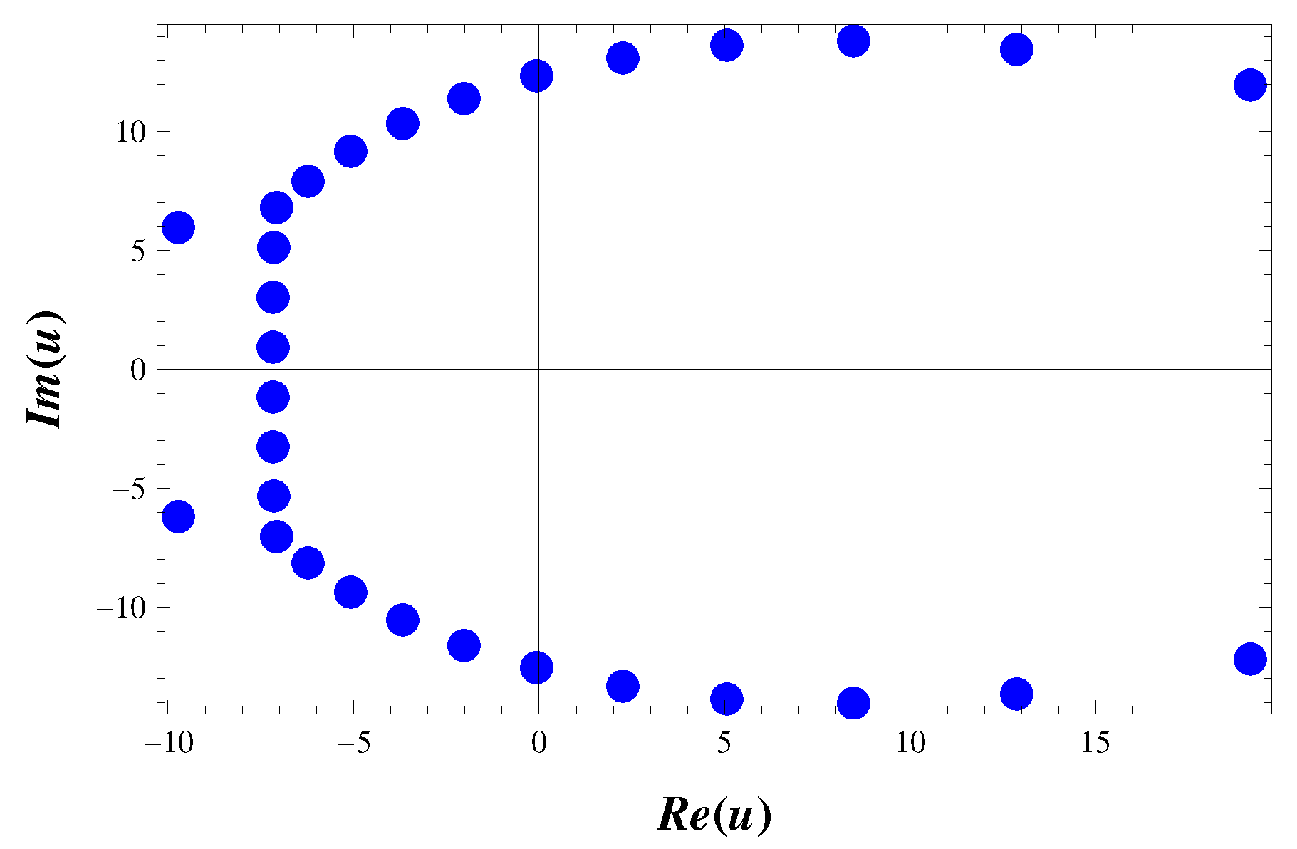
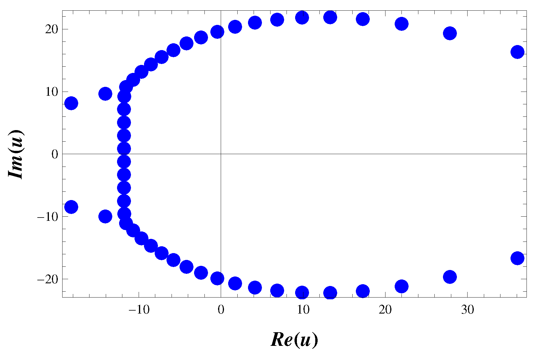
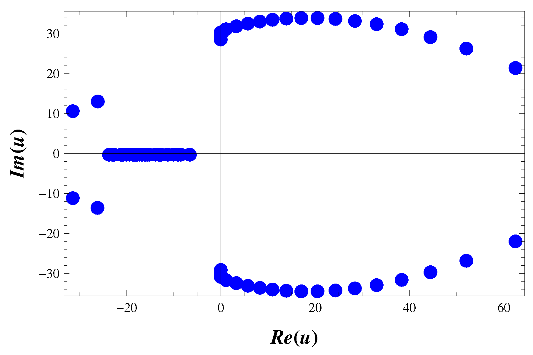
All possible zeros of ${}_e{\mathcal{C}}_n^{*}\left(u\right)$ $(n\in \mathbb{N})$ are located in symmetric places with respect to the real axis.

Indeed, let $u_0\in \mathbb{C}$ be a zero of ${}_e{\mathcal{C}}_n^{*}\left(u\right)$. Then

$$0=\overline{0}=\overline{{}_e{\mathcal{C}}_n^{*}\left(u_0\right)}=\sum _{k=0}^n\sum _{r=0}^k\frac{{(-1)}^{n-k}{\overline{u_0}}^r}{2^{n-k}r!}={}_e{\mathcal{C}}_n^{*}\left(\overline{u_0}\right),$$

where $\overline{u}$ denotes the conjugate of $u\in \mathbb{C}$. This implies that $\overline{u_0}$ is also a zero of ${}_e{\mathcal{C}}_n^{*}\left(u\right)$.

(ii)

The polynomial ${}_e{\mathcal{C}}_n^{*}\left(u\right)$ in (57) is a polynomial in the variable u of degree n, all of whose coefficients are positive rational numbers. So, ${}_e{\mathcal{C}}_n^{*}\left(u\right)$ $(n\in \mathbb{N})$ has n zeros, counting multiplicities, in the finite complex plane. Explicitly,

$${}_e{\mathcal{C}}_n^{*}\left(u\right)=\sum _{r=0}^n{c}_r\left(n\right)u^r,$$

(58)

where

$$c_r\left(n\right)=\frac{2}{3·r!}\left(1+\frac{{(-1)}^{n-r}}{2^{n-r+1}}\right).$$

(59)

In particular,

$$c_0\left(n\right)=\frac{2}{3}\left(1+\frac{{(-1)}^n}{2^{n+1}}\right)\mathrm{and}{c}_n\left(n\right)=\frac{1}{n!}.$$

Indeed, we can rewrite (57) as follows:

$${}_e{\mathcal{C}}_n^{*}\left(u\right)=\sum _{r=0}^n{c}_r\left(n\right)u^r,$$

$$c_r\left(n\right)=\sum _{k=r}^n\frac{{(-1)}^{n-k}}{2^{n-k}r!},$$

where $n,r\in {\mathbb{N}}_0$ are such that $0\le r\le n$. The right-handed series of $c_r\left(n\right)$ is a geometric series with common ratio $-2$, the first term ${(-1)}^{n-r}/(2^{n-r}r!)$, and the number of terms $n-r+1$. We thus have the above explicit expression (58) with (59). The first statement follows immediately from this explicit expression. The second one is implied by fundamental theorem of algebra (see, e.g., ([61], p. 1), ([41], p. 77)).

(iii)

We have observed the 78 graphs of zeros of the polynomials ${}_e{\mathcal{C}}_n^{*}\left(u\right)$ from $n=3$ to $n=80$. We choose to demonstrate only 9 graphs as below Figure 1, Figure 2, Figure 3, Figure 4, Figure 5, Figure 6, Figure 7, Figure 8 and Figure 9.

In view of those graphs, we find the followings:

(a)

If ${}_e{\mathcal{C}}_n^{*}\left(u\right)$ = 0, then $|\Im \left(u\right)|<\frac{n}{2}+1$ $(n\in \mathbb{N})$.

(b)

If ${}_e{\mathcal{C}}_n^{*}\left(u\right)$=0, then $-\frac{n}{2}<|\Re \left(u\right)|<n$ $(n\in \mathbb{N})$.

(c)

The number of zeros of ${}_e{\mathcal{C}}_n^{*}\left(u\right)$ with $\Re \left(u\right)>0$ is less than the number of zeros of ${}_e{\mathcal{C}}_n^{*}\left(u\right)$ with $\Re \left(u\right)<0$ when $n\ge 5$.

(d)

The longest straight distance from the origin of zeros of ${}_e{\mathcal{C}}_n^{*}\left(u\right)$ with $\Re \left(u\right)>0$ is greater than that of zeros of ${}_e{\mathcal{C}}_n^{*}\left(u\right)$ with $\Re \left(u\right)<0$, when $n\ge 3$. That is,

$$sup\left\{\left|u\right||{}_e{\mathcal{C}}_n^{*}\left(u\right)=0,\Re \left(u\right)>0\right\}>sup\left\{\left|u\right||{}_e{\mathcal{C}}_n^{*}\left(u\right),=0,\Re \left(u\right)<0\right\}.$$

where $n\ge 3$.

(iv)

[Approximation of the real zero of ${}_e{\mathcal{C}}_n^{*}\left(x\right)$ $(n\ge 3)$

In view of (i) and (ii) in this section, the polynomials ${}_e{\mathcal{C}}_{2n+1}^{*}\left(x\right)$ $\left(n\in {\mathbb{N}}_0\right)$ are found to have one real zero. ${}_e{\mathcal{C}}_n^{*}\left(x\right)$ $(n\in \mathbb{N},x\in \mathbb{R})$ are real-valued infinitely differentiable functions on the interval $(-\infty ,\infty )$. Indeed, here, only twice differentiability is sufficient. To approximate the real zeros of ${}_e{\mathcal{C}}_{2n+1}^{*}\left(x\right)$, we can use Newton–Raphson’s theorem (see, e.g., [58], pp. 262–263). We try to apply this theorem to find the real zero of the polynomial

$${}_e{\mathcal{C}}_3^{*}\left(x\right)=\frac{x^3}{6}+\frac{x^2}{4}+\frac{3x}{4}+\frac{5}{8}.$$

First set $x=-1$ in ${}_e{\mathcal{C}}_3^{*}\left(x\right)$ to get ${}_e{\mathcal{C}}_3^{*}(-1)=-\frac{1}{24}=-0.0416...$. We see that $x=-1$ is very near at the real zero c, say. Let $x_0=-1$. Then consider the sequence $x_n$ $(n\in \mathbb{N})$ given by

$$x_n=x_{n-1}-\frac{{}_e{\mathcal{C}}_3^{*}\left(x_{n-1}\right)}{\frac{\mathrm{d}}{\mathrm{d}x}{}_e{\mathcal{C}}_3^{*}\left(x_{n-1}\right)}=x_{n-1}-\frac{4x_{n-1}^3+6x_{n-1}^2+18x_{n-1}+15}{12x_{n-1}^2+12x_{n-1}+18}.$$

From this recursive relation, we compute

$$x_1==-0.9444...,x_2=-0.943417831...,x_3=-0.943417508210...,x_4=-0.943417507926...$$

From this, we may guess that the sequence $\left\{x_n\right\}$ is increasing and converges to the real zero $c=-0.94341750...$ as $n\to \infty$.

7. Conclusions, Remarks, and Open Questions

The so-called truncated-exponential-based Appell-type Changhee polynomials ${}_e{\mathcal{C}}_n^{*}\left(x\right)$ were introduced. Then certain properties and identities for these new polynomials, such as explicit representation, addition formulas, recurrence relations, differential and integral formulas, and some related inequalities, are presented, together with some integral inequalities involving these polynomials. The Hermite–Hadamard type inequality (see (54)) captivated many researchers who have produced a large number of interesting inequalities of this type including its diverse generalizations (see, e.g., [57,62] and the references cited therein).

In Section 6, zero distributions of the polynomials ${}_e{\mathcal{C}}_n^{*}\left(u\right)$ $(3\le n\le 80)$ have been observed, experimentally, by using graphs. From (58) and (59), we write the polynomials ${}_e{\mathcal{C}}_n^{*}\left(u\right)$ in polar form

$${}_e{\mathcal{C}}_n^{*}\left(u\right)=\sum _{r=0}^n{c}_r{\left(n\right)\left|u\right|}^r{\mathrm{e}}^{r\theta }=\sum _{r=0}^n{c}_r{\left(n\right)\left|u\right|}^{r}cos\left(r\theta \right)+i\sum _{r=0}^n{c}_r\left(n\right){\left|u\right|}^{r}sin\left(r\theta \right),$$

(60)

where $i=\sqrt{-1}$.

Questions:

(i)

All of the zeros of ${}_e{\mathcal{C}}_n^{*}\left(u\right)$ $(1\le n\le 80)$ are observed to be simple, that is, all the zeros are distinct. Are the zeros of ${}_e{\mathcal{C}}_n^{*}\left(u\right)$, when $n\in \mathbb{N}$ is greater than 80, are distinct?

(ii)

Can the observations (a), (b), (c), and (d) in Section 6 as well as some other ones (if any) be generalized when $n\in \mathbb{N}$ is greater than 80?.

(iii)

From (60), how can we determine (or approximate) $\left|u\right|$ and $\theta$ such that

$${}_e{\mathcal{C}}_n^{*}\left(u\right)=0\iff \sum _{r=0}^n{c}_r{\left(n\right)\left|u\right|}^{r}cos\left(r\theta \right)=0=\sum _{r=0}^n{c}_r\left(n\right){\left|u\right|}^{r}sin\left(r\theta \right),$$

(61)

for $n\in \mathbb{N}\backslash \left\{1\right\}$?

For example, since $\frac{1\pm \sqrt{5}i}{2}$ are zeros of ${}_e{\mathcal{C}}_2^{*}\left(u\right)$, $\left|u\right|=\sqrt{3}/2$ and $\theta =arctan\sqrt{5}$ satisfy

$$\sum _{r=0}^2{c}_r{\left(2\right)\left|u\right|}^{r}cos\left(r\theta \right)=0=\sum _{r=0}^2{c}_r\left(2\right){\left|u\right|}^{r}sin\left(r\theta \right).$$

We may apply Newton–Raphson’s method in (iv), Section 6, to real and imaginary parts of the right-most side of (60) (or (61)), respectively, to approximate complex zeros of ${}_e{\mathcal{C}}_n^{*}\left(u\right)$.

Further properties, applications, and theoretical investigation of distributions of zeros of the polynomials ${}_e{\mathcal{C}}_n^{*}\left(u\right)$ introduced here are left to the authors and the interested researchers, for future study.

References

- Bayad, A.; Hamahata, Y. Poly-Euler polynomials and Arakawa-Kaneko type zeta functions. Funct. Approx. Comment. Math. 2014, 51, 7–22. [Google Scholar]
- Dattoli, G.; Cesarano, C.; Sacchetti, D. A note on truncated polynomials. Appl. Math. Comput. 2003, 134, 595–605. [Google Scholar] [CrossRef]
- Khan, S.; Nahid, T. Finding non-linear differential equations and certain identities for the Bernoulli-Euler and Bernoulli-Genocchi numbers. SN Appl. Sci. 2019, 1, 217. [Google Scholar] [CrossRef]
- Khan, N.; Usman, T.; Choi, J. A new class of generalized polynomials. Turk. J. Math. 2018, 42, 1366–1379. [Google Scholar]
- Kim, T. p-adic q-integrals associated with the Changhee-Barnes’ q-Bernoulli polynomials. Integral Transform. Spec. Funct. 2004, 15, 415–420. [Google Scholar] [CrossRef]
- Kim, T.; Kim, D.S. Differential equations associated with Catalan-Daehee numbers and their applications. RACSAM 2017, 111, 1071–1081. [Google Scholar] [CrossRef]
- Kim, T.; Kim, D.S.; Kwon, H.I.; Seo, J.J. Revisit nonlinear differential equations associated with Bernoulli numbers of the second kind. Glob. J. Pure Appl. Math. 2016, 12, 1893–1901. [Google Scholar]
- Kim, D.S.; Kim, T.; Seo, J.J. A note on Changhee polynomials and numbers. Adv. Stud. Theor. Phys. 2013, 7, 993–1003. [Google Scholar] [CrossRef]
- Kim, D.S.; Kim, T.; Seo, J.J.; Lee, S.-H.; Schork, M. Higher-order Changhee numbers and polynomials. Adv. Stud. Theor. Phys. 2014, 8, 365–373. [Google Scholar] [CrossRef][Green Version]
- Kim, T.; Kim, D.S. A note on nonlinear Changhee differential equations. Russ. J. Math. Phys. 2016, 23, 88–92. [Google Scholar] [CrossRef]
- Kurt, B. Notes on the poly-Korobov type polynomials and related polynomials. Filomat 2020. accepted. [Google Scholar]
- Kurt, V. On the generalized q-poly-Euler polynomials of second kind. Filomat 2020. accepted. [Google Scholar]
- Kurt, B.; Simsek, Y. Notes on generalization of the Bernoulli type polynomials. Appl. Math. Comput. 2011, 218, 906–911. [Google Scholar] [CrossRef]
- Lee, J.G.; Jang, L.-C.; Seo, J.-J.; Choi, S.-K.; Kwon, H.I. On Appell-type Changhee polynomials and numbers. Adv. Differ. Equ. 2016, 2016, 160. [Google Scholar] [CrossRef][Green Version]
- Luo, Q.M.; Guo, B.N.; Qi, F.; Debnath, L. Generalization of Bernoulli numbers and polynomials. Int. J. Math. Math. Sci. 2003, 61, 3769–3776. [Google Scholar] [CrossRef]
- Ozden, H.; Cangul, I.N.; Simsek, Y. Generalized q-Stirling numbers and their interpolation functions. Axioms 2013, 2, 10–19. [Google Scholar] [CrossRef]
- Simsek, Y. New families of special numbers for computing negative order Euler numbers and related numbers and polynomials. Appl. Anal. Discret. Math. 2018, 12, 1–35. [Google Scholar] [CrossRef]
- Wang, N.L.; Li, H. Some identities on the higher-order Daehee and Changhee numbers. Pure Appl. Math. J. 2015, 5, 33–37. [Google Scholar]
- Andrews, L.C. Special Functions for Engineers and Applied Mathematicians; Macmillan Publishing Company: New York, NY, USA, 1985. [Google Scholar]
- Schur, I. Einige Sätze über primzahlen mit anwendungen auf irreduzibilitätsfragen I. Sitzungsberichte Preuss. Akad. Wiss. Phys.-Math. Klasse 1929, 125–136, Also in Gesammelte Abhandlungen, Band III, 140–151. [Google Scholar]
- Schur, I. Einige Sätze über primzahlen mit anwendungen auf irreduzibilitätsfragen II. Sitzungsberichte Preuss. Akad. Wiss. Phys.-Math. Klasse 1929, 370–391, Also in Gesammelte Abhandlungen, Band III, 152–173. [Google Scholar]
- Coleman, R. On the Galois groups of the exponential Taylor polynomials. Enseign. Math. 1987, 33, 183–189. [Google Scholar]
- Erdös, P. A theorem of Sylvester and Schur. J. Lond. Math. Soc. 1934, 9, 282–288. [Google Scholar] [CrossRef]
- Ali, M.; Khan, S. Finding results for certain relatives of the Appell polynomials. Bull. Korean Math. Soc. 2019, 56, 151–167. [Google Scholar] [CrossRef]
- Araci, S.; Riyasat, M.; Nahid, T.; Khan, S. Certain results for unified Apostol type-truncated exponential-Gould-Hopper polynomials and their relatives. arXiv 2006, arXiv:2006.12970v1. [Google Scholar]
- Barakat, R. Evaluation of the incomplete Gamma function of imaginary argument by Chebyshev polynomials. Math. Comput. 1961, 15, 7–11. [Google Scholar] [CrossRef]
- Belingeri, C.; Dattoli, G.; Khan, S.; Ricci, P.E. Monomiality and multi-index multi-variable special polynomials. Integral Transforms Spec. Funct. 2007, 18, 449–458. [Google Scholar] [CrossRef]
- Choi, J.; Jabee, S.; Shadab, M. Some identities associated with 2-variable truncated exponential based Sheffer polynomial sequences. Commun. Korean Math. Soc. 2020, 35, 533–546. [Google Scholar] [CrossRef]
- Chung, W.S.; Hassanabadi, H. Truncated exponential polynomials and truncated coherent states. Eur. Phys. J. Plus 2020, 135, 556. [Google Scholar] [CrossRef]
- Dattoli, G.; Migliorati, M. The truncated exponential polynomials, the associated Hermite forms and applications. Int. J. Math. Math. Sci. 2006, 2006, 98175. [Google Scholar] [CrossRef]
- Dattoli, G.; Ricci, P.E.; Marinelli, L. Generalized truncated exponential polynomials and applications. Rend. Istit. Mat. Univ. Trieste 2002, 34, 9–18. [Google Scholar]
- Dattoli, G.; Torre, A.; Carpanese, M. The Hermite-Bessel functions: A new point of view on the theory of generalized Bessel functions. Radiat. Phys. Chem. 1998, 3, 221–228. [Google Scholar]
- Gori, F. Flattened Gaussian beams. Opt. Commun. 1994, 107, 335–341. [Google Scholar] [CrossRef]
- Joung, H. Asymptotic expansions of recursion coefficients of orthogonal polynomials with truncated exponential weights. Nagoya Math. J. 2002, 165, 79–89. [Google Scholar] [CrossRef][Green Version]
- Khan, S.; Yasmin, G.; Ahmad, N. On a new family related to truncated exponential and Sheffer polynomials. J. Math. Anal. Appl. 2014, 418, 921–937. [Google Scholar] [CrossRef]
- Khan, S.; Yasmin, G.; Ahmad, N. A Note on truncated exponential-based Appell polynomials. Bull. Malays. Math. Sci. Soc. 2017, 40, 373–388. [Google Scholar] [CrossRef]
- Kumam, W.; Srivastava, H.M.; Wani, S.A.; Araci, S.; Kumam, P. Truncated-exponential-based Frobenius-Euler polynomials. Adv. Differ. Equ. 2019, 2019, 530. [Google Scholar] [CrossRef]
- Srivastava, H.M.; Araci, S.; Khan, W.A.; Acikgöz, M. A note on the truncated-exponential based Apostol-type polynomials. Symmetry 2019, 11, 538. [Google Scholar] [CrossRef]
- Srivastava, H.M.; Choi, J. Zeta and q-Zeta Functions and Associated Series and Integrals; Elsevier Science Publishers: Amsterdam, The Netherlands; London, UK; New York, NY, USA, 2012. [Google Scholar]
- Lim, D.; Qi, F. On the Appell type λ-Changhee polynomials. J. Nonlinear Sci. Appl. 2016, 9, 1872–1876. [Google Scholar] [CrossRef]
- Conway, J.B. Functions of One Complex Variable, 2nd ed.; Springer: New York, NY, USA; Berlin/Heidelberg, Germany, 1978. [Google Scholar]
- Appell, P. Sur une classe de polynômes. Ann. Sci. École Norm. Sup. 1880, 9, 119–144. [Google Scholar] [CrossRef]
- Boas, R.P.; Buck, R.C. Polynomial Expansions of Analytic Functions; Springer: Berlin/Heidelberg, Germany, 1964. [Google Scholar]
- Bretti, G.; Cesarano, C.; Ricci, P.E. Laguerre-type exponential and generalized Appell polynomials. Comput. Math. Appl. 2004, 48, 833–839. [Google Scholar] [CrossRef]
- Bretti, G.; He, M.X.; Ricci, P.E. On quadrature rules associated with Appell polynomials. Int. J. Appl. Math. 2002, 11, 1–14. [Google Scholar]
- Bretti, G.; Natalini, P.; Ricci, P.E. Generalizations of the Bernoulli and Appell polynomials. Abstr. Appl. Anal. 2004, 7, 613–623. [Google Scholar] [CrossRef]
- Bretti, G.; Ricci, P.E. Multidimensional extensions of the Bernoulli and Appell polynomials. Taiwanese J. Math. 2004, 8, 415–428. [Google Scholar] [CrossRef]
- Dattoli, G.; Ricci, P.E.; Cesarano, C. Differential equations for Appell type polynomials. Fract. Calc. Appl. Anal. 2002, 5, 69–75. [Google Scholar]
- Douak, K. The relation of the d-orthogonal polynomials to the Appell polynomials. J. Comput. Appl. Math. 1996, 70, 279–295. [Google Scholar] [CrossRef]
- He, M.X.; Ricci, P.E. Differential equation of Appell polynomials via the factorization method. J. Comput. Appl. Math. 2002, 139, 231–237. [Google Scholar] [CrossRef]
- Ismail, M.E.H. Remarks on differential equation of Appell polynomials via the factorization method. J. Comput. Appl. Math. 2003, 154, 243–245. [Google Scholar] [CrossRef]
- Roman, S. The Umbral Calculus; Academic Press: New York, NY, USA, 1984. [Google Scholar]
- Sheffer, I.M. A differential equation for Appell polynomials. Bull. Am. Math. Soc. 1935, 41, 914–923. [Google Scholar] [CrossRef][Green Version]
- Shohat, J. The relation of the classical orthogonal polynomials to the polynomials of Appell. Am. J. Math. 1936, 58, 453–464. [Google Scholar] [CrossRef]
- Szegö, G. Orthogonal Polynomials; American Mathematical Society: Providence, RI, USA, 1939. [Google Scholar]
- Hardy, G.H.; Littlewood, J.E.; Pólya, G. Inequalities, 2nd ed.; Cambridge University Press: Cambridge, UK, 2001. [Google Scholar]
- Set, E.; Choi, J.; Çelık, B. Certain Hermite–Hadamard type inequalities involving generalized fractional integral operators. RACSAM 2018, 112, 1539–1547. [Google Scholar] [CrossRef]
- Wade, W.R. An Introduction to Analysis, 4th ed.; Pearson Education: Upper Saddle River, NJ, USA, 2010. [Google Scholar]
- Kuijlaars, A.B.J.; Assche, W.V. The asymptotic zero distribution of orthogonal polynomials with varying recurrence coefficients. J. Approx. Theor. 1999, 99, 167–197. [Google Scholar] [CrossRef]
- Martínez-Finkelshteina, A.; Martínez-González, P.; Orive, R. On asymptotic zero distribution of Laguerre and generalized Bessel polynomials with varying parameters. J. Comput. Appl. Math. 2001, 133, 477–487. [Google Scholar] [CrossRef][Green Version]
- Sheil-Small, T. Complex Polynomials; Cambrige University Press: Cambridge, UK, 2002. [Google Scholar]
- Dragomir, S.S.; Pearce, C.E.M. Selected Topics on Hermite–Hadamard Inequalities and Applications; RGMIA Monographs; Victoria University: Melbourne, Australia, 2000. [Google Scholar]
© 2020 by the authors. Licensee MDPI, Basel, Switzerland. This article is an open access article distributed under the terms and conditions of the Creative Commons Attribution (CC BY) license (http://creativecommons.org/licenses/by/4.0/).
Share and Cite
Nahid, T.; Alam, P.; Choi, J. Truncated-Exponential-Based Appell-Type Changhee Polynomials. Symmetry 2020, 12, 1588. https://doi.org/10.3390/sym12101588
Nahid T, Alam P, Choi J. Truncated-Exponential-Based Appell-Type Changhee Polynomials. Symmetry. 2020; 12(10):1588. https://doi.org/10.3390/sym12101588
Chicago/Turabian StyleNahid, Tabinda, Parvez Alam, and Junesang Choi. 2020. "Truncated-Exponential-Based Appell-Type Changhee Polynomials" Symmetry 12, no. 10: 1588. https://doi.org/10.3390/sym12101588
APA StyleNahid, T., Alam, P., & Choi, J. (2020). Truncated-Exponential-Based Appell-Type Changhee Polynomials. Symmetry, 12(10), 1588. https://doi.org/10.3390/sym12101588