A Fast and Exact Greedy Algorithm for the Core–Periphery Problem

Abstract

The core–periphery structure is one of the key concepts in the structural analysis of complex networks. It consists of a partitioning of the node set of a given graph or network into two groups, called core and periphery, where the core nodes induce a well-connected subgraph and share connections with peripheral nodes, while the peripheral nodes are loosely connected to the core nodes and other peripheral nodes. We propose a polynomial-time algorithm to detect core–periphery structures in networks having a symmetric adjacency matrix. The core set is defined as the solution of a combinatorial optimization problem, which has a pleasant symmetry with respect to graph complementation. We provide a complete description of the optimal solutions to that problem and an exact and efficient algorithm to compute them. The proposed approach is extended to networks with loops and oriented edges. Numerical simulations are carried out on both synthetic and real-world networks to demonstrate the effectiveness and practicability of the proposed algorithm.

1. Introduction

The structural analysis of graphs and networks found in the real world aims at extracting high-level features or summarizing relevant properties of large data sets. That analysis can be carried out at different levels, depending on specific goals and viewpoints. A microscopic, node-level analysis intends to discover which network elements are most relevant for e.g., network cohesion and functioning, information or epidemic diffusion, or flow control. At the other extreme, one may want to concisely describe a quantitative property of a given network by one or a few numbers, for example, the overall number of nodes or edges and the average node degree, which quantify how large is a network and how strongly is connected, respectively.

A third approach to network analysis, which lies in between these two extremes, is the so-called network clustering or block-modeling [1,2,3]. Roughly speaking, it consists of detecting the presence of various types of intermediate structures, typically consisting of groups of nodes that exhibit very specific patterns of relationships in their interior and with the rest of the network. For instance, a group of nodes that is rich in internal connections but is loosely connected with the exterior can be identified as a community. Community detection problems have received considerable attention in the network science literature because communities emerge naturally in many social, biological, or collaboration networks [3,4]. Besides communities, other network structures can be recognized and are attracting considerable interest nowadays. For example, in the analysis of biological networks including predator and prey species or social networks with ties representing hostilities, an important task is the identification of anti-communities, namely, groups of nodes being poorly connected internally but having many links between different groups. Communities and anti-communities may coexist, for instance in communication and social networks, giving rise to nested block structures that are difficult to disentangle [1,5,6].

Another block structure recurring in the analysis of complex networks is the core–periphery structure, whose investigation has been popularized by the seminal works by Borgatti and Everett [7]. In the last two decades the interest toward core–periphery structures had a remarkable growth in the network science literature [6,8,9,10]. In its simplest form, a core–periphery structure can be described as a partitioning of a given graph or network into two groups of nodes, called core and periphery. The core nodes are tightly interconnected and share connections with peripheral nodes, while peripheral nodes are loosely connected to core nodes and to other peripheral nodes. The presence of core–periphery structures has been detected in a large variety of complex systems, such as social networks, trade networks, and financial networks, see e.g., [9,11,12].

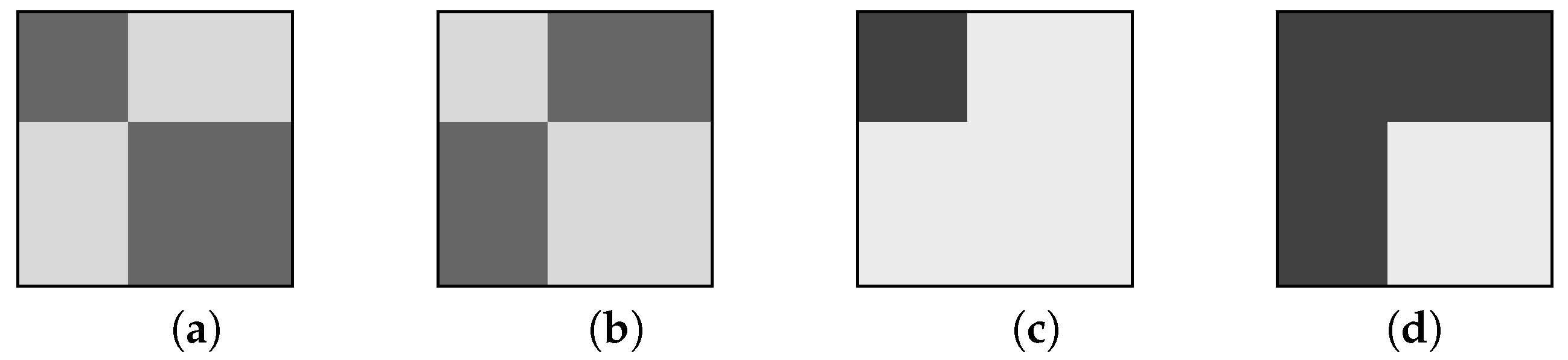
These network structures are well described by means of suitable block partitionings of an adjacency matrix representing idealized situations [1,2,3]. Various basic mesoscale network structures that can be described by a block partitioning of the adjacency matrix are illustrated in Figure 1. Darker shadings represent matrix blocks having more nonzero entries, and denote the presence of stronger connections between the corresponding node sets. These idealized block structures can be identified by a variety of statistical and matrix analysis tools, give a reasonable approximation of structured real-world networks and can be easily reproduced synthetically.

Figure 1. Examples of 2-block models for various mesoscale structures in undirected graphs. Shaded areas represent densities of non-zero entries in idealized adjacency matrices. (a) A block model with two communities. (b) A block model with two anti-communities. (c,d) The two prototypical core–periphery block models introduced in [7].

In this paper, we address the case where a core–periphery structure is present in a given graph and must be discovered. We consider a core–periphery bipartitioning method considered by Brusco in [13]. This method is based on a block model where off-diagonal blocks are neglected, and identifies the core nodes as belonging to a subset that minimizes a certain objective function. Our main result is an algorithm that exactly solves that combinatorial optimization problem with a computational cost that grows at most quadratically in the number of nodes. This significantly improves the computational time required to solve the problem with respect to the branch-and-bound procedure proposed in [13]. The combination of computational efficiency and theoretical justification makes our algorithm attractive for the analysis of large networks.

In the next section, we introduce the combinatorial optimization problem we adopt to define the core–periphery partitioning and derive an exact algorithm to solve it. Since that problem may have multiple optimal solutions, we also provide a complete description of the optimal solution set and show a pleasant symmetry in our approach with respect to graph complementation. At first, we consider the core–periphery partitioning problem in loopless graphs whose adjacency matrix is symmetric. In Section 3 we extend our optimization approach to graphs with loops and to directed graphs. Section 4 is devoted to applications of our methodology to two real-world networks and two graph families that are relevant to complex network analysis, that is, equitable graphs and power-law networks.

1.1. Related Work

Core–periphery models are basically divided into discrete and continuous models. Discrete models induce a binary classification of the nodes as belonging either to the core, which has a high edge density, or to the periphery, whose edge density is low. The sought partitioning is determined by maximizing a correlation index or other matrix nearness measures between the adjacency matrix and an idealized block structure, see e.g., [12,13,14,15]. In continuous models each node obtains a value describing its “coreness”; unlike in discrete models, that value is a real, positive number. Continuous models may be based on a matrix similarity criterion, analogously to discrete models [6,10], or on a node-level centrality index quantifying the extent to which a vertex controls the information that flows through the network. To the latter class belong various bipartitioning algorithms based on closeness or betweenness indices [9,14] and other measurements based on random walks [11,16]. Both continuous and discrete models have been pioneered by Borgatti and Everett [7]. They proposed two prototypical block structures for core–periphery partitionings, namely, those depicted in Figure 1c,d. The basic assumption is that every two core nodes are directly connected while peripheral nodes have no direct links. Connections between core nodes and peripheral nodes may be requested (see Figure 1c) or not (see Figure 1d). Recent reviews on modeling and analyzing core–periphery structures, together with the related concepts of degree assortativity, rich-clubs, and nested network structures, can be found in [6,8,14,16].

1.2. Notation

For the purposes of this work, we borrow some basic notions from graph theory [4,17]. A graph or network G consists of a finite set V of nodes or vertices and a set E of edges. Each edge $e\in E$ is an unordered pair of nodes. If $e=\{i,j\}$ then we say that nodes i and j are adjacent, and that e is incident to both i and j. For notational simplicity, we identify V with $\{1,2,\dots ,n\}$ and we denote by $ij$ the edge $\{i,j\}$. Note that $ij=ji$. A complete graph is a graph in which all nodes are adjacent to each other. In some cases, it is useful to admit the presence of loops, that is, edges having the form $ii$. Unless otherwise specified, we mainly consider simple graphs, i.e., graphs without loops and parallel edges, that is, edges incident to the same node pair.

A weighted graph is a graph endowed with an edge weight, that is a function $w:E\mapsto \mathbb{R}$ assigning a real (usually positive) number to every edge. We denote $w_{ij}$ the weight of the edge $ij$. Clearly, $w_{ij}=w_{ji}$.

The adjacency matrix of a simple graph G with n nodes is the $n\times n$ symmetric matrix $A=(a_{ij})$ such that $a_{ij}=1$ if $ij$ is an edge in G and $a_{ij}=0$ otherwise. If the graph is weighted then $a_{ij}=w_{ij}$ if $ij$ is an edge in G and $a_{ij}=0$ otherwise. For $i=1,\dots ,n$ define

$$d_i=\sum _{j=1}^n{a}_{ij}.$$

In an unweighted graph $d_i$ is the degree of node i, that is, the number of edges incident to it. If the graph is weighted, then the number $d_i$ is usually called strength or generalized degree of i. It represents the total weight of edges incident to i, and may not be an integer. In what follows, we simply call $d_i$ the degree of node i, both in weighted and unweighted graphs.

The sets $S_1,\dots ,S_{\ell }$ form a partition of V if ${\cup }_{k=1}^{\ell }{S}_k=V$ and $S_i\cap S_j=⌀$ for $i\ne j$. The cardinality of a subset $S\subseteq V$ is denoted by $\left|S\right|$, and the complementary set $V\setminus S$ by $\overline{S}$. The pair $\{S,\overline{S}\}$ is a bipartition of V. The subgraph induced by S is the graph $G^{\prime }=(S,E^{\prime })$ where $ij\in E^{\prime }$ iff $ij\in E$ and $\{i,j\}\subseteq S$. Equivalently, if A is the adjacency matrix of G then the adjacency matrix of $G^{\prime }$ is the submatrix of A extracted from rows and columns with indices in S. Finally, the volume of $S\subseteq V$ is

$$\mathrm{vol}(S)=\sum _{i\in S}{d}_i=\sum _{i\in S}\sum _{j=1}^n{a}_{ij}.$$

2. Identifying a Core–Periphery Bipartition

Let $G=(V,E)$ be a weighted graph and let A be its adjacency matrix. We assume that every edge $ij\in E$ is endowed with a positive weight $0<w_{ij}\le 1$, so that the entries of A belongs to the interval $[0,1]$. We may think of $a_{ij}$ as a relative measure, or fraction, of the strength of the interaction between nodes i and j with respect to a maximal capacity: If $a_{ij}=1$ then the bond between the two nodes is perfect, or as strong as possible, while if $a_{ij}=0$ then the two nodes do not interact; all intermediate values between these two extremes can be allowed. Obviously, this assumption includes trivially the case where the graph to be considered is unweighted, in which case $w_{ij}=1$ for every $ij\in E$.

In this section, we address the problem of identifying a core–periphery bipartition of G that we suppose to exist in the graph. Note that we are not considering the problem of deciding whether or not that bipartition actually exists, that is, measuring the statistical significance of that structure, which is a different problem considered in, e.g., [9,11]. For the moment, we restrict ourselves to the case where G has no loops or they must be ignored if present, as is common in most network applications. Consider the following function defined over subsets of V:

$$z(S)=\sum _{\begin{array}{c}i,j\in S\\ i\ne j\end{array}}(1-a_{ij})+\sum _{\begin{array}{c}i,j\notin S\\ i\ne j\end{array}}{a}_{ij},S\subseteq V.$$

(1)

The first term counts the overall weight that is missing in the subgraph induced by S with respect to the ideal situation where all node pairs are perfectly connected, while the second term is the overall weight of edges that are present in the subgraph induced by the complementary set $\overline{S}$. Thus, if $z(S)$ is close to zero then S can be recognized as a core in the graph since its nodes are tightly connected to each other; at the same time, the nodes in $\overline{S}$ induce a subgraph with few or no edges, hence $\overline{S}$ represents a peripheral zone of the network. Therefore, the localization of a core–periphery structure in G can be carried out by looking for a set $S\subseteq V$ attaining a minimal value of $z(S)$. In the sequel we will analyze the following combinatorial optimization problem, also considered in [13]:

$$\underset{S\subseteq V}{min}z(S).$$

(2)

2.1. A Greedy Algorithm for Problem (2)

For any vertex set $S\subseteq V$ define the following auxiliary quantities:

• the overall weight of the edges in the subgraph induced by S is $e(S)={\sum }_{i,j\in S}{a}_{ij}$
• the overall weight of the edges having exactly one node in S is $\partial (S)={\sum }_{i\in S}{\sum }_{j\notin S}{a}_{ij}$.

It is immediate to see that $\mathrm{vol}(S)=e(S)+\partial (S)$. Moreover, owing to the symmetry of A, we have $\partial (S)=\partial (\overline{S})$. Hence the function $z(S)$ can be rewritten as follows:

$$\begin{array}{cc}\hfill z(S)& =\left|S\right|(|S|-1)-e(S)+e(\overline{S})\hfill \\ \hfill & =\left|S\right|(|S|-1)-\mathrm{vol}(S)+\partial (S)+\mathrm{vol}(\overline{S})-\partial (\overline{S})\hfill \\ \hfill & =\left|S\right|(|S|-1)-\mathrm{vol}(S)+\mathrm{vol}(\overline{S})\hfill \\ \hfill & =\left|S\right|(|S|-1)+\mathrm{vol}(V)-2\mathrm{vol}(S).\hfill \end{array}$$

The last passage comes from the identity $\mathrm{vol}(S)+\mathrm{vol}(\overline{S})=\mathrm{vol}(V)$.

Observe that Problem (2) can be restated equivalently as

$$\underset{k=1,\dots ,n}{min}\underset{\begin{array}{c}S\subseteq V\\ \left|S\right|=k\end{array}}{min}z(S).$$

With this restatement we can reduce the solution of Problem (2) to that of at most n subproblems endowed with a cardinality constraint. Finding a set $S\subseteq V$ that minimizes $z(S)$ having a prescribed cardinality is an easy task. In fact, owing to the previous arguments, if $\left|S\right|=k$ then $z(S)=k(k-1)+v-2\mathrm{vol}(S)$, where $v=\mathrm{vol}(V)={\sum }_{i,j}{a}_{ij}$ is the overall weight of edges in G. However, since v does not depend on k, its presence is unessential in the solution of Problem (2), and an optimal solution of the k-th subproblem consists of a set S with cardinality k and maximum volume. Such set can be easily computed by the greedy strategy described here below.

Without loss of generality, we can assume that the nodes of G are numbered in non-increasing order of their degrees:

$$d_1\ge d_2\ge \dots \ge d_n.$$

(3)

Then, for each given $k=\left|S\right|$, a set which minimizes $z(S)$ is $S=\{1,\dots ,k\}$. Consequently, the optimal value of $z(S)$ under the constraint $\left|S\right|=k$ is given by

$$z_k:=\underset{\begin{array}{c}S\subseteq V\\ \left|S\right|=k\end{array}}{min}z(S)=k(k-1)+v-2\sum _{i=1}^k{d}_i.$$

Finally, denoting by $z^{\ast }$ the optimal value of Problem (2), it holds $z^{\ast }={min}_k{z}_k$. Letting ${\sigma }_k=z_k-v$, we have the equivalent characterization $z^{\ast }=v+{min}_k{\sigma }_k$. In conclusion, Problem (2) can be solved by the following three-step procedure:

• For $i=1,\dots ,n$ compute the degrees $d_i={\sum }_j{a}_{ij}$ and reorder the nodes in non-increasing order by degree, as in Formula (3).
• For $k=1,\dots ,n$ let ${\sigma }_k=k(k-1)-2{\sum }_{i=1}^k{d}_i$.
• Let $k^{\ast }$ be an integer such that ${\sigma }_{k^{\ast }}={min}_k{\sigma }_k$. Then the optimal value of Problem (2) is $z^{\ast }=z_{k^{\ast }}$ and the set $S^{\ast }=\{1,\dots ,k^{\ast }\}$ is an optimal solution to Problem (2).

The computation of the optimal index $k^{\ast }$ can be simplified by noting that the numbers

$${\Delta }_k:={\sigma }_k-{\sigma }_{k-1}=2(k-1)-2d_k$$

form a strictly increasing sequence:

$${\Delta }_{k+1}-{\Delta }_k=2+2(d_k-d_{k+1})\ge 2.$$

(4)

This implies that the sequence ${\sigma }_1,\dots ,{\sigma }_n$ is convex, and its minimum is attained at the largest integer $k^{\ast }$ such that ${\Delta }_{k^{\ast }}<0$. Hence, the step 2 in the preceding procedure needs to be performed only as long as ${\Delta }_k<0$, that is, $d_k>k-1$. In summary, the previous procedure can be better described by the Algorithm 1 here below, which provides an optimal solution to Problem (2). This fact, and the possible existence of other optimal solutions, is formalized in the subsequent results.

Algorithm 1: Computing an optimal solution of Problem (2)

Input: symmetric adjacency matrix $A=(a_{ij})$ of size n Output: integer $k^{\ast }$, core set $S^{\ast }$ Compute a permutation $\pi$ of $\{1,\dots ,n\}$ such that $d_{\pi (1)}\ge d_{\pi (2)}\ge \dots \ge d_{\pi (n)}$ $k\leftarrow 1$ $k^{\ast }\leftarrow k$ Define the core set $S^{\ast }=\{\pi (1),\dots ,\pi (k^{\ast })\}$

Theorem 1.

Under the node ordering Formula (3), let $k^{\ast }$ be the integer defined as

$$k^{\ast }=max\{k\in \{1,\dots ,n\}:d_k>k-1\}.$$

(5)

Then, Problem (2) has an optimal solution having cardinality $k^{\ast }$, that is,

$$\underset{S\subseteq V}{min}z(S)=z_{k^{\ast }}.$$

One such optimal solution is given by $S^{\ast }=\{1,\dots ,k^{\ast }\}$. That solution is the unique optimal solution with cardinality $k^{\ast }$ if and only if $d_{k^{\ast }}>d_{k^{\ast }+1}$.

Proof. 

The fact that $S^{\ast }$ solves Problem (2) has been shown by the previous arguments. In fact, the inequality $d_k>k-1$ appearing in Equation (5) is equivalent to the condition ${\Delta }_k={\sigma }_k-{\sigma }_{k-1}<0$. Note that that condition cannot be replaced by $d_k\ge k$ since $d_k$ may not be an integer if the graph G is weighted. Uniqueness holds if and only if there is exactly one way to choose $k^{\ast }$ nodes whose degree is not smaller than $d_{k^{\ast }}$, that is, $d_{k^{\ast }}>d_{k^{\ast }+1}$.  □

Remark 1.

The integer $k^{\ast }$ in Equation (5) can be defined equivalently as the smallest integer k such that ${\Delta }_{k+1}={\sigma }_{k+1}-{\sigma }_k\ge 0$. Since ${\sigma }_{k+1}-{\sigma }_k=2(k-d_{k+1})$, we have the following alternative characterization:

$$k^{\ast }=min\{k\in \{1,\dots ,n-1\}:d_{k+1}\le k\}.$$

(6)

Corollary 1.

Every optimal solution to Problem (2) has cardinality either $k^{\ast }$ or $k^{\ast }+1$. Moreover, an optimal solution of cardinality $k^{\ast }+1$ exists if and only if $d_{k^{\ast }+1}=k^{\ast }$.

Proof. 

Since the optimal value of Problem (2) is $z_{k^{\ast }}=v+{\sigma }_{k^{\ast }}$, there exists an optimal solution $S^{\prime }$ with $|S^{\prime }|=\ell >k^{\ast }$ if and only if ${\sigma }_{k^{\ast }}={\sigma }_{\ell }$. In that case, if $\ell =k^{\ast }+1$ then we obtain

$$0={\sigma }_{k^{\ast }}-{\sigma }_{k^{\ast }+1}=2d_{k^{\ast }+1}-2k^{\ast }.$$

So the identity $d_{k^{\ast }+1}=k^{\ast }$ is equivalent to the existence of a solution $S^{\prime }$ with $|S^{\prime }|=k^{\ast }+1$. To prove that no solution with cardinality larger than $k^{\ast }+1$ can exist it is sufficient to observe that from Equation (4) for any k we get

$$2\le {\Delta }_{k+1}-{\Delta }_k={\sigma }_{k+1}-2{\sigma }_k+{\sigma }_{k-1}.$$

Hence the identity ${\sigma }_{k^{\ast }}={\sigma }_{k^{\ast }+1}={\sigma }_{k^{\ast }+2}$ is impossible.  □

In conclusion, assuming that the degree sequence $d_1,\dots ,d_n$ is ordered as in Formula (3), the optimal solution set of Problem (2) falls into one of the following alternatives:

• If $d_{k^{\ast }}>d_{k^{\ast }+1}$ and $d_{k^{\ast }+1}<k^{\ast }$ then $S^{\ast }=\{1,\dots ,k^{\ast }\}$ is the unique optimal solution.
• If $d_{k^{\ast }}>d_{k^{\ast }+1}$ and there exists an integer $h\ge 1$ such that $k^{\ast }=d_{k^{\ast }+1}=\dots =d_{k^{\ast }+h}$ then both $S^{\ast }=\{1,\dots ,k^{\ast }\}$ and $S^{\ast }\cup \{k^{\ast }+i\}$ are optimal solutions, for every $i=1,\dots ,h$.
• If there exists an integer $h\ge 1$ such that $d_{k^{\ast }}=\dots =d_{k^{\ast }+h}$ then the problem is solved by any set made by either $k^{\ast }$ or $k^{\ast }+1$ vertices whose degree is not smaller than $d_{k^{\ast }}$ and containing all the vertices whose degree is greater than $d_{k^{\ast }}$.

Example 1.

Consider the following simple graphs:

In both graphs the nodes are already ordered according to Formula (3), and we have $k^{\ast }=2$. In $G_1$, Problem (2) has three optimal solutions, namely $\{1,2\}$, $\{1,3\}$ and $\{1,2,3\}$, since the uniqueness condition $d_2>d_3$ in Theorem 1 is broken and $d_3=2$. In $G_2$ we have $d_3=d_4=2$, hence Corollary 1 indicates the existence of solutions having cardinality 2 and 3. Moreover, the smallest solution is unique, since $d_2>d_3$. In fact, the solutions are $\{1,2\}$, $\{1,2,3\}$ and $\{1,2,4\}$.

Remark 2.

The computational cost (in terms of elementary arithmetic-logical operations) of Algorithm 1 can be analyzed as follows.

1. 

If the matrix A is given in a sparse format or, equivalently, the graph G is represented by an adjacency list, the degrees $d_1,\dots ,d_n$ can be computed in $\mathcal{O}(m)$ operations where m is the number of edges in G. In any case, that cost is not larger than $\mathcal{O}(n^2)$.

2. 

Standard sorting algorithms can reorder the numbers $d_i$ in non-increasing order in $\mathcal{O}(nlogn)$ operations, in the worst case.

3. 

The computation of the integer $k^{\ast }$ in Equation (5) requires no more than $\mathcal{O}(n)$ operations.

Thus, Algorithm 1 requires $\mathcal{O}(m+nlogn)$ operations, that is $\mathcal{O}(n^2)$ operations in the worst case. We point out that the complexity of the branch-and-bound algorithm in [13] to solve Problem (2) is unknown, but the timings reported in that paper suggest an exponential behavior in n.

2.2. A Symmetry Property

The formalization of the core–periphery problem proposed in Problem (2) has a pleasant symmetry with respect to graph complementation. Given a loopless graph $G=(V,E)$ with adjacency matrix $A=(a_{ij})$ let $G^{\prime }=(V,E^{\prime })$ be its complementary graph, that is, the graph whose adjacency matrix is $A^{\prime }=(a_{ij}^{\prime })$ where

$$a_{ij}^{\prime }=\left\{\begin{array}{cc}1-a_{ij}\hfill & i\ne j\hfill \\ 0\hfill & i=j.\hfill \end{array}\right.$$

(7)

If G is unweighted then any two distinct vertices are adjacent in $G^{\prime }$ if and only if they are not adjacent in G. It is not hard to see that if S is a core for G then $\overline{S}$ is a core for $G^{\prime }$. Indeed, let $z_G(S)$ and $z_{G^{\prime }}(S)$ be the function z in Equation (1) computed in G and $G^{\prime }$, respectively. Then, from Equation (7) we have

$$\begin{array}{cc}\hfill z_{G^{\prime }}(S)& =\sum _{\begin{array}{c}i,j\in S\\ i\ne j\end{array}}(1-a_{ij}^{\prime })+\sum _{\begin{array}{c}i,j\notin S\\ i\ne j\end{array}}{a}_{ij}^{\prime }\hfill \\ \hfill & =\sum _{\begin{array}{c}i,j\in S\\ i\ne j\end{array}}{a}_{ij}+\sum _{\begin{array}{c}i,j\notin S\\ i\ne j\end{array}}(1-a_{ij})=z_G(\overline{S}).\hfill \end{array}$$

Thus, S is a solution of Problem (2) in G if and only if $\overline{S}$ solves Problem (2) in $G^{\prime }$.

3. Allowing Loops and Directed Edges

In this section we extend the core–periphery partitioning algorithm discussed previously to two different settings. Firstly, we consider the case where loops are present and must be taken into consideration; afterwards, we address directed graphs, that is, graphs where node adjacency relationships are unsymmetric.

3.1. Allowing Loops

Certain networks include loops, that is, edges of the form $ii$, which must be taken in due consideration in the structural analysis of the network. In that case, some diagonal entries of the adjacency matrix are nonzero. In fact, it is customary to set $a_{ii}=1$ in the adjacency matrix of an unweighted graph when the loop $ii$ is present in the graph. In order to tackle appropriately the presence of loops, it is reasonable to modify the Definition (1) by including the contribution of the diagonal entries of A in the summations. Hereafter, we sketch briefly the consequent changes in the solution of the corresponding optimization Problem (2) with respect to the previous paragraphs.

• Following the same arguments considered in the loopless case, the expression of $z(S)$ becomes

  $$z(S)={\left|S\right|}^2+v-2\mathrm{vol}(S),v=\sum _{i,j}{a}_{ij}.$$
• The optimal value of $z(S)$ under the constraint $\left|S\right|=k$ is given by $z_k=k^2+v-2(d_1+\cdots +d_k)$, and the index $k^{\ast }$ characterizing the (least) cardinality of a core is

  $$\begin{array}{cc}\hfill k^{\ast }& =max\{k\in \{1,\dots ,n\}:d_k>k-1/2\}\hfill \\ \hfill & =min\{k\in \{1,\dots ,n-1\}:d_{k+1}\le k+1/2\}.\hfill \end{array}$$

Anyway, the symmetry property described in the previous paragraph continues to hold. Indeed, when loops are allowed, the adjacency matrix of the complementary graph is $A^{\prime }=(a_{ij}^{\prime })$ with $a_{ij}^{\prime }=1-a_{ij}$.

3.2. Directed Graphs

A directed graph, or digraph, differs from a graph in that the incidence relation is unsymmetric. For definiteness, a directed graph is a pair $G=(V,E)$ where V is a set of vertices or nodes and $E\subseteq V\times V$. Hence, any element $e\in E$ is an ordered pair of nodes, $e=(i,j)$, called directed edge or arc. In this paragraph we consider directed unweighted graphs, so the adjacency matrix of G is the matrix $A=(a_{ij})$ such that $a_{ij}=1$ if $(i,j)\in E$ and $a_{ij}=0$ otherwise. In a directed graph, loops are usually admitted.

The identification of a core–periphery partitioning in a directed graph can be carried out by extending to the present setting the principle adopted in the undirected case. That is, we argue that core nodes should form a well-connected subset, inducing a subgraph that is as most complete as possible, while the number of arcs running between peripheral nodes should be kept as small as possible. In our approach, the number of arcs between core nodes and peripheral nodes is unimportant. This principle can be formalized as follows. Let A be the adjacency matrix of a directed graph G. We define the core of G as a set $S\subseteq V$ which minimizes the objective function

$$z(S)=\sum _{i,j\in S}(1-a_{ij})+\sum _{i,j\notin S}{a}_{ij}.$$

(8)

Hereafter, we describe how the optimization of this function can be carried out with the help of the algorithm devised in the previous section.

Suppose we are given the adjacency matrix A of a directed unweighted graph $G=(V,E)$, and let $B=\frac{1}{2}(A+A^T)$. We can think of $B=(b_{ij})$ as the adjacency matrix of an undirected graph $G^{\prime }=(V,E^{\prime })$ having the same vertex set of the original graph and where each edge $ij\in E^{\prime }$ is endowed by a weight $w_{ij}$ whose value is either 1 or $\frac{1}{2}$. In fact, when $i\ne j$ we have $b_{ij}=1$ iff both $ij\in E$ and $ji\in E$, while $b_{ij}=\frac{1}{2}$ iff exactly one of $ij\in E$ and $ji\in E$ is true. Obviously, $b_{ij}=0$ means that both edges $ij$ and $ji$ are absent in G (and in $G^{\prime }$, too). Also loops in G and $G^{\prime }$ are the same, since $a_{ii}=b_{ii}$. Moreover, for any subset $S\subseteq V$ we have the identity ${\sum }_{i,j\in S}{a}_{ij}={\sum }_{i,j\in S}{b}_{ij}$. Finally, note that if every arc in G has its own reciprocal, that is $ij\in E\iff ji\in E$, then A is symmetric and $A=B$.

Hence, for any $S\subseteq V$, the value of $z(S)$ computed in the directed graph G via Equation (8) is the same as the value of $z(S)$ computed in the symmetrised and weighted graph $G^{\prime }$. Thus the only modification needed in the algorithm in the preceding section to deal with directed graphs is to define the numbers $d_i$ as

$$d_i=\sum _{j=1}^n{b}_{ij}=\frac{1}{2}\sum _{j=1}^n(a_{ij}+a_{ji}).$$

The computation of the solution $S^{\ast }$ can be carried out as outlined in the previous paragraph.

4. Examples

In this section, we discuss the application of our bipartitioning algorithm to two real-world networks that are popular benchmarks for graph blockmodel problems, and to two graph families often encountered as idealized models of complex networks, namely, the equitable graphs and the graphs having a power-law degree profile.

4.1. Two Real-World Networks

In this paragraph, we report the results of the application of Algorithm 1 to two real-world networks that are available in the Pajek network repository [18].

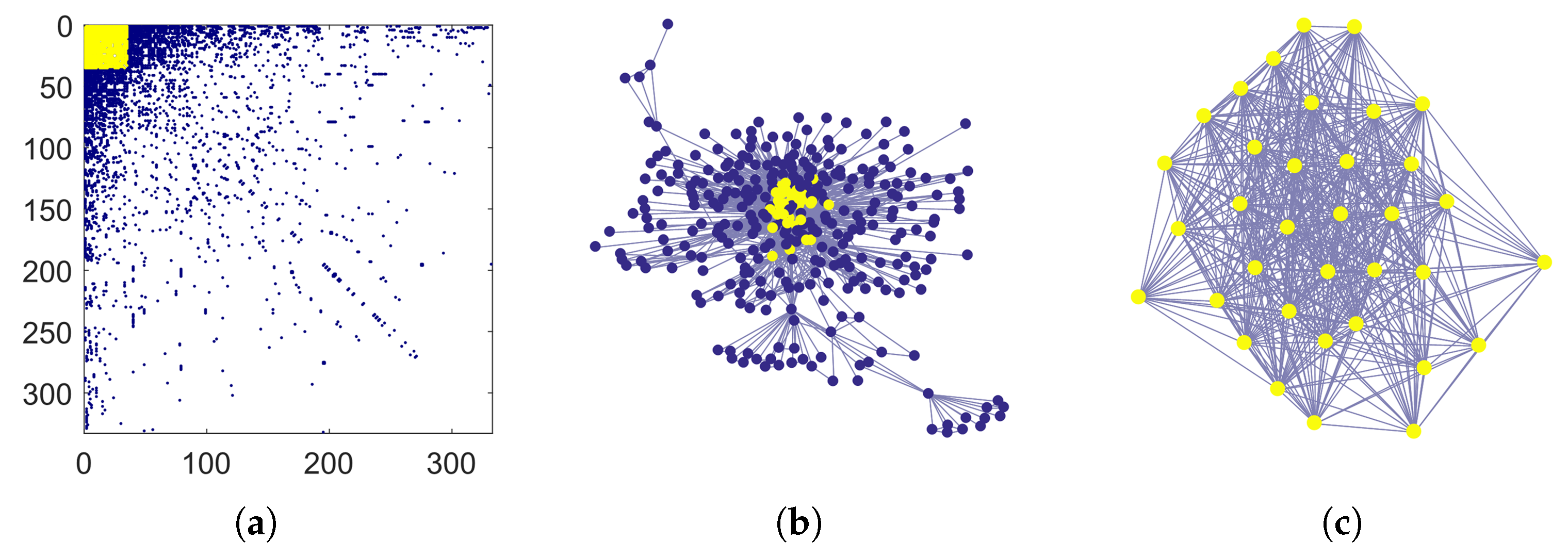
The USAir97 dataset is a graph built from the USA national aerial flights in 1997. Each node represents an airport, and two nodes are connected by an undirected edge if the corresponding airports are served by a direct flight in either direction. The graph has 332 nodes and 2126 edges, so the average degree is about $12.8$. Algorithm 1 identifies as core a well connected set of $k^{\ast }=35$ nodes. The left panel in Figure 2 shows the adjacency matrix once the nodes have been reordered according to their degree, as in Equation (3). Colored dots are placed in correspondence with nonzero matrix entries. The matrix entries corresponding to the core nodes are shown in yellow. That submatrix is very dense, due to the fact that the subgraph induced by core nodes has 505 edges and the average degree in that subgraph is about $28.9$. A graphical layout of USAir97 is shown in the central panel in Figure 2, where core nodes are colored in yellow. The subgraph induced by the core nodes is displayed in the right panel. Incidentally, we note that in this example Problem (2) has also an optimal solution with 36 nodes, since $d_{35}=36$, $d_{36}=35$ and $d_{37}=34$.

Figure 2. Core–periphery bipartition of the network USAir97. (a) The adjacency matrix, reordered according to the node numbering in Formula (3); entries in the core block are shown in yellow. (b) A graphical layout of the network. Core nodes are shown in yellow. (c) The subgraph induced by core nodes.

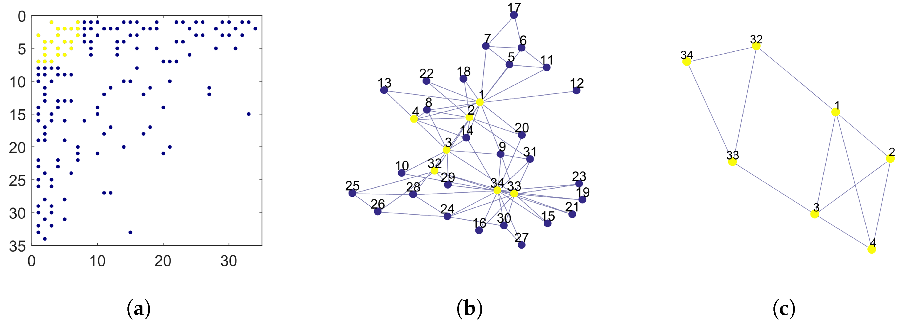
The Zachary dataset represents a small social network made by members of a karate club [19]. The graph has 34 nodes and 78 edges representing ties among club members. This network is one of the most widely used testbeds for community detection algorithms. Here below, we compare the core identified by Algorithm 1 in this network with those identified by other algorithms in the recent literature [15,16]. For this network, Problem (2) has two optimal solutions with six nodes and one optimal solution with seven nodes. We consider the latter as core in the following discussion. The left panel in Figure 3 shows the pattern of the adjacency matrix after nodes are rearranged in non-increasing order by degree. Yellow dots mark the position of the non-zero entries in the core block. The central panel represents a graphical layout of the network. Each node is marked by its original node number to allow comparisons with related works, as shown in Table 1. Core nodes are marked in yellow. The rightmost panel represents the subgraph induced by the core nodes. Finally, Table 1 collects the results of Algorithm 1 together with those by three core–periphery partitioning algorithms presented in [15] (called BE-KL, 2-step, and divisive) and the rich-core algorithm in [16]. For each algorithm, we list the core nodes identified by it by their original node numbers. It is worth noting that, according to the analysis presented in [15], the Zachary network actually contains two distinct communities comprising a large part of the network, each community having an internal core–periphery structure.

Figure 3. Core–periphery bipartition of the network Zachary. (a) The adjacency matrix, reordered according to the node numbering in Formula (3); entries in the core block are shown in yellow. (b) A graphical layout of the network. Core nodes are shown in yellow. Node numbering as in the original graph. (c) The subgraph induced by core nodes.

Table 1. Core nodes identified in the Zachary network by different algorithms.

Algorithm 1	BE-KL [15]	2-step [15]	Divisive [15]	Rich-core [16]
$1,2,3,4,32,33,34$	$1,2,3,33,34$	$1,2,4,33,34$	$1,2,3,4,24,33,34$	$1,2,3,4,9,14,24,32,33,34$

4.2. Equitable Graphs

Let $G=(V,E)$ be a graph with adjacency matrix A. A partition $\{V_1,\dots ,V_{\ell }\}$ of V is equitable if there exists an $\ell \times \ell$ matrix $P=(p_{ij})$, called the partition matrix, such that for all $h,k=1,\dots ,\ell$,

$$\forall i\in V_h,\sum _{j\in V_{\ell }}{a}_{ij}=p_{hk}.$$

(9)

Simply put, every node in the h-th block is connected with exactly $p_{hk}$ nodes in the k-th block. In that case, the graph G is called equitable with respect to the given partition. The subsets $V_1,\dots ,V_{\ell }$ are the blocks of the graph. For the Equation (9) to have solution, the entries of the partition matrix must fulfill the identities

$$|V_i|p_{ij}=\left|V_j\right|p_{ji},i,j=1,\dots ,\ell .$$

Equitable graphs have been used in many problems in combinatorics, algebraic graph theory, and community detection problems [20,21]. They represent the deterministic counterpart of the stochastic block models, which are random graphs where the probability that two nodes are adjacent depends on their block indices [1,2,3].

The idealized core–periphery structures introduced in [7] and shown in Figure 1c,d are defined by equitable graphs with two blocks.

Let G be an equitable graph with respect to the partition $\{V_1,\dots ,V_{\ell }\}$ and let P be the partition matrix. Note that the degree of a node depends only on its block index. Indeed, let $\beta (i)$ denote the block index of node $i\in V$. Then, $d_i={\sum }_{j=1}^{\ell }{p}_{\beta (i),j}$. Thus if $\beta (i)=\beta (j)$ then $d_i=d_j$. The goal of this paragraph is to analyze to what extent the core–periphery algorithm proposed here recognizes the nodes with largest degree as core nodes in an equitable graph. For $i=1,\dots ,\ell$ let $d^{(i)}={\sum }_{j=1}^{\ell }{p}_{ij}$ be the degree of each node in $V_i$. We assume $d^{(1)}>d^{(i)}$ for $i>1$.

Hence, the candidate core nodes are those in the first block. The following result describes the relationship between $V_1$ and the core set identified by the proposed algorithm.

Corollary 2.

In the hypotheses stated above, let $n_1=\left|V_1\right|$.

1. 

If $d^{(1)}\le n_1$ then every optimal solution of Problem (2) is a subset of $V_1$,

2. 

if $d^{(1)}\ge n_1$ then every optimal solution of Problem (2) contains $V_1$ as subset.

Proof. 

Assume, without loss in generality, that the nodes are ordered as in Formula (3). Let $k^{\ast }$ be the index defined in Equation (5) and let $S^{\ast }=\{1,\dots ,k^{\ast }\}$.

• If $d^{(1)}\le n_1$ then

  $$d_{d^{(1)}}=d^{(1)}>d^{(1)}-1,d_{d^{(1)}+1}\le d_{d^{(1)}}=d^{(1)}.$$
  Owing to Equations (5) and (6) we have $k^{\ast }=d^{(1)}\le n_1$ and consequently $S^{\ast }\subseteq V_1$. To prove that every other optimal solution is included in $V_1$ it remains to show that if $k^{\ast }=n_1$ then no optimal solution can have $k^{\ast }+1$ nodes. By Corollary 1 an optimal solution with cardinality $k^{\ast }+1$ exists if and only if $d_{k^{\ast }+1}=k^{\ast }$, but if $k^{\ast }=n_1$ then $d_{k^{\ast }+1}<d^{(1)}=k^{\ast }$ and we are done.
• If $n_1\le d^{(1)}$ then $d_{n_1}=d^{(1)}>n_1-1$. Hence $k^{\ast }\ge n_1$ and $V_1\subseteq S^{\ast }$.  □

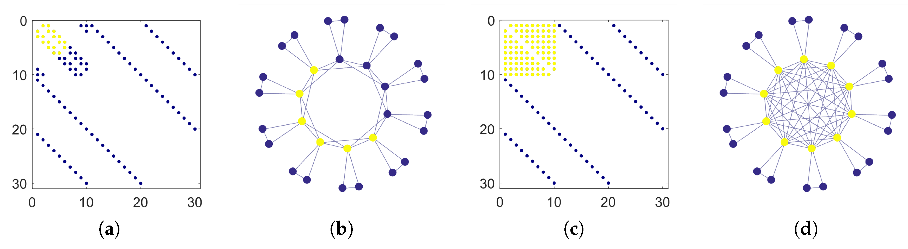
Figure 4 shows the adjacency matrices and the graphical layouts of two equitable graphs with $n=30$, $\ell =3$ and $|V_1|=|V_2|=|V_3|=10$. Letting

$$P(a)=\left(\begin{array}{ccc}a& 1& 1\\ 1& 0& 1\\ 1& 1& 0\end{array}\right),$$

(10)

the associated partition matrices are $P(4)$ (leftmost panels) and $P(9)$ (rightmost panels), respectively. As in the preceding paragraph, the core nodes identified by Algorithm 1 are marked in yellow. When $a=4$ the core is a proper subset of the first block, due to its scarce internal density. In fact, in this case we have $d^{(1)}=6$ and $d^{(2)}=d^{(3)}=2$. In the other case $d^{(1)}=11$, $d^{(2)}=d^{(3)}=2$, the subgraph induced by the first block is complete and the core coincides exactly with the first block.

Figure 4. Core–periphery bipartition of two equitable graphs with $n=30$ and three blocks. The partition matrices are $P(4)$ (a,b) and $P(9)$ (c,d), respectively, where $P(a)$ is given in Equation (10). Yellow dots correspond to core nodes, according to Algorithm 1.

Remark 3.

The two idealized core–periphery structures introduced by Borgatti and Everett (in the loopless case), which are depicted in Figure 1c,d, correspond to equitable graphs with a 2-block partition $\{V_1,V_2\}$ and the two partition matrices

$$P_1=\left(\begin{array}{cc}{n}_1-1& 0\\ 0& 0\end{array}\right),P_1=\left(\begin{array}{cc}{n}_1-1& n_1\\ n_2& 0\end{array}\right),$$

respectively, where $n_i=\left|V_i\right|$ for $i=1,2$. The following are immediate consequences of Corollary 2.

• In the first case we have $d_{n_1-1}=n_1-1>n_1-2$ while $d_{n_1}=n_1-1<n_1$. Hence $k^{\ast }=n_1-1$ and the set $S^{\ast }$ identified by our algorithm is $V_1$ except one node. However, since $d_{n_1}=k^{\ast }$, from Corollary 1 we obtain that also $V_1$ is a solution of Problem (2).
• In the second case we have $d_{n_1}=n-1>n_1-1$ while $d_{n_1+1}=n_1\le n_1$. Also in this case $k^{\ast }=n_1$ and $V_1$ is a core. However, we also have $d_{n_1+1}=n_1$. Hence by Corollary 1 any set having the form $V_1\cup \left\{i\right\}$ with $i\in V_2$ is also a solution of Problem (2).

4.3. Power-Law Networks

A graph or network is considered to have a power-law degree distribution with exponent $\gamma$ if the number $n_k$ of nodes having degree k is approximately given by $\alpha k^{-\gamma }$, where $\alpha$ is a coefficient that depends on the size of the graph ([4] Chap. 4). Many interesting real-world networks have a power-law degree distribution with an exponent $\gamma \in (2,3)$. In fact, power-law degree distributions arise naturally in networks evolving in time by the addition of new nodes and edges according to the so-called preferential attachment rules, see e.g., ([4] Chap. 6) or ([17] Chap. 3). For that reason, a power-law network is usually intended as belonging to a sequence of networks with increasing sizes having a power-law degree distribution whose exponent $\gamma$ is independent on the network size.

Power-law networks are often deemed as having a core–periphery structure [9,17]. In this paragraph we examine the outcome of our bipartitioning algorithm when applied to power-law networks. The next result describes the asymptotic behavior of the core identified by Algorithm 1 when the network size n diverges. In what follows, the notation $f(n)\approx g(n)$ means that $f(n)/g(n)\to 1$ as $n\to \infty$.

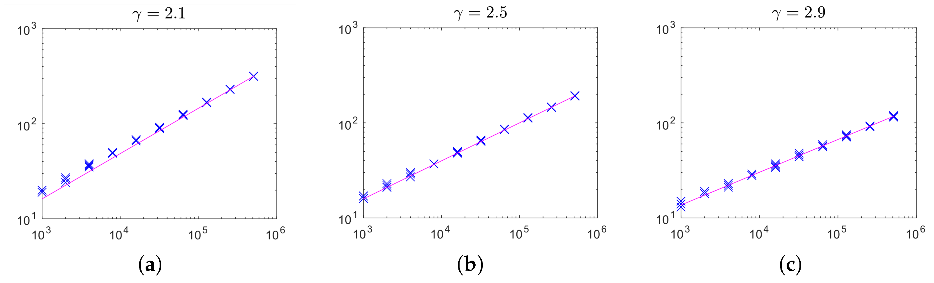
Corollary 3.

Let G be a power-law network with exponent $\gamma >2$ and no isolated nodes. Assuming that the average degree in G does not depend on n, the number of nodes in the core set is $\mathcal{O}(n^{1/\gamma })$.

Proof. 

Let $n_k\approx \alpha k^{-\gamma }$ be the degree profile of G, where $\alpha$ depends on n. For $k\ge 1$ let $N(k)$ be the number of nodes with degree greater than or equal to k. With these notations, the integer $k^{\ast }$ in Equation (5) can be characterized by the identity

$$k^{\ast }=\left|\{i:d_i\ge k^{\ast }\}\right|=N(k^{\ast }).$$

For large n, the number $N(k)$ can be approximated by

$$N(k)=\sum _{i=k}^{\infty }{n}_i\approx \alpha {\int }_k^{\infty }{x}^{-\gamma }\mathrm{d}x=\frac{\alpha }{\gamma -1}{k}^{1-\gamma }.$$

(11)

Let $d_{min}$ and $d_{max}$ be the smallest and largest degree in G, respectively. The average degree $d_{\mathrm{avg}}$ in G is

$$d_{\mathrm{avg}}=\frac{1}{n}\sum _{k=d_{min}}^{d_{max}}N(k)\approx \frac{\alpha }{n(\gamma -1)}{\int }_{d_{min}}^{d_{max}}{k}^{1-\gamma }=\frac{C\alpha }{n(\gamma -1)(\gamma -2)},$$

where $C=d_{min}^{2-\gamma }-d_{max}^{2-\gamma }$. By hypotheses, C is bounded above and below by positive constants, hence we have $\alpha =\mathcal{O}(n)$, since $d_{\mathrm{avg}}$ does not depend on n. By Equation (11), we can estimate $k^{\ast }$ as the solution of the equation $k=\alpha k^{1-\gamma }/(\gamma -1)$, that is,

$$k^{\ast }={\left(\frac{\alpha }{1-\gamma }\right)}^{1/\gamma },$$

and the claim follows.  □

To validate experimentally the claim of the previous corollary, we performed a series of simulations with power-law networks generated by means of the algorithm described in [22]. That algorithm generates random graphs in the Chung–Lu model [17], which is a flexible, very popular random graph model with nice theoretical properties. We generated random power-law networks with size $n=1000·2^{i-1}$ for $i=1,\dots ,10$ and average degree equal to 3, in expectation. In Figure 5, we display the core size versus the network size for networks with exponent $\gamma =2.1$ (left), $\gamma =2.5$ (center) and $\gamma =2.9$ (right). Each cross represents the result for one network. The solid lines plot functions $\kappa n^{1/\gamma }$ where $\kappa$ is chosen to fit the results obtained with the largest size n. As is clearly visible, the core sizes approach very closely the theoretical behavior estimated in Corollary 3 over a very large range of n.

Figure 5. Core sizes in power-law networks generated by the Chung–Lu random graph model. Horizontal axes: size n of a power-law network with average degree 3. Vertical axes: number of nodes in the corresponding core. Each cross represents a random network. Solid lines show the $\mathcal{O}(n^{1/\gamma })$ behavior. (a) $\gamma =2.1$; (b) $\gamma =2.5$; (c) $\gamma =2.9$.

5. Conclusions

In a variety of complex real-world systems that are modeled as networks, one often observes the presence of a group of densely interconnected nodes, while the remaining nodes form a sparse peripheral area with few internal links. This particular pattern is called core–periphery, and is one of the key mesoscopic structures that are relevant to the analysis of complex networks.

In this work we proposed a fast and theoretically well-founded algorithm for the localization of core–periphery structures in both oriented and non-oriented complex networks, assuming the presence of that structure. Basically, the set of core nodes is identified by a certain combinatorial optimization problem that has been introduced earlier by Brusco in [13]. We provided a complete description of the set of optimal solutions to that optimization problem. Our algorithm has a very low computational cost, both in terms of memory space and operation count, which makes it suitable for the analysis of large networks. The applicability of the algorithm has been demonstrated experimentally on both real-world and synthetic networks.