1. Introduction
The concepts of reliability and safety have been integral to technical systems, as a rule. However, according to recent reviews in reliability engineering, technical systems should be considered in environments, taking the human factor into account to improve the accuracy of reliability or safety evaluations [
1,
2]. This can complicate the mathematical models of investigated systems (objects) because the mathematical representation of systems under study is an integral part of reliability analysis. Mathematical representations map component states into system states and are used to compute reliability indices and measures for system evaluations. There are many types of mathematical representations, such as fault trees [
3], reliability block diagrams [
4], structure functions [
4,
5], Markov models [
6], Petri nets [
7], Bayesan belief networks [
8,
9], credal networks [
10,
11], survival signatures [
12] and others. The choice and use one of these representations depends on application problems and the specifics of risk/reliability analysis. Mathematical representations in the form of a fault tree, reliability block diagram or structure function re more suitable for systems in which the causal implications of the failure/success of a component is well identified and deterministic. Advantages of these mathematical representations are simplicity and the possibility to be constructed for a system of any structure complexity [
13], but new methods need to be developed for their application in time-dependent reliability analysis, such using a survival signature [
12,
14], credal network [
11,
15] or other method [
16]. Markov models or Monte Carlo simulations can be accepted for time-depend (dynamic) analysis of system reliability [
6,
15]. The probabilistic models are used for the mathematical representation in cases of incompletely specified or uncertain data for analysis and relationships among system components that cannot be represented deterministically [
2,
9]. Many practical problems cannot be determined based on only one of these mathematical representations, and require the development and application of hybridized mathematical representations. Human reliability analysis (HRA) has often been used as one such mathematical representation [
9,
14,
17].
HRA methods are typically developed for analyzing nuclear power plant operations and transport control [
18,
19]. HRA methods and tools allow the analysis of potential failures in human interactions with complex socio-technical systems, and the evaluation of personnel failure and the factors influenced by it [
9,
20]. According to [
21], HRA methods can be divided into three generations. Methods of all these generations are alternative and successfully complement each other. Methods of the first generation allow predicting and quantifying human error in terms of success/failure of the action, with less attention to the depth of the causes and reasons behind the human behavior. Examples of such methods are the human error assessment and reduction technique (HEART) [
22] or the Success Likelihood Index Method (SLIM) [
23]. The second generation HRA methods are conceptual types that take into account the cognitive aspects of humans and the causes of errors rather than their frequency. The Cognitive Reliability and Error Analysis Method (CREAM) is often considered to be a second-generation method [
24]. The third generation agrees with the simulation-based HRA methods that allow reductions of uncertainties in the information used to conduct human reliability assessments. Nuclear action reliability assessment (NARA) can be considered an example of this generation method, and is an advanced version of HEART for the nuclear field [
19]. Incompleteness and uncertainty of relevant data is typical in HRA, and expert judgment is used extensively to compensate for a lack of data. This specific relevant data causes the development of new methods based on hybrid probabilistic mathematical models [
21,
25,
26]. In particular, a Bayesian belief network-based method is developed in [
20] for nuclear power plants, and in [
23] for handling uncertainty arising from experts’ opinions and absent data, while methods applying fuzzy logic are considered in [
27,
28] and a multi-state-system-based mathematical model is used for human error probability evaluation in [
29]. The application of hybrid mathematical representations in HRA methods compensates for incompleteness and uncertainty of relevant data.
As a rule, newly developed mathematical models need new methods to evaluate and calculate human error probability, along with other measures. At the same time, there are many measures for examining systems and their components in reliability engineering, with various methods for their calculation. These methods can be explored if a mathematical model is typical (e.g., it is a fault tree or structure function). However, such mathematical representations can be used for deterministic descriptions of problems for reliability analysis that are not possible in HRA. The development of new methods for constructing the structure function that are based on uncertain data can allow the use of a traditional model of the structure function in HRA. In this paper, we propose the application of a new method for constructing the structure function based on uncertain data in HRA, and use it to evaluate systems while considering the human factor. An important novelty of the proposed method is the interpretation of the structure function as a classification structure. The proposed method permits the uncertainty of relevant data to be taken into account as the result of two factors [
30]. The first of these factors is ambiguity and vagueness of collected data, which can be caused by an inaccuracy or error of measurement or expert judgment. The transformation of initial data into fuzzy data can take into account this uncertainty [
31]. The second factor is the incompleteness of data in rare system states [
2,
31,
32], which can be recovered by, for example, a decision tree [
33,
34]. In this study, we used the algorithm for fuzzy decision tree FDT induction proposed in [
35]. The decision table can be constructed based on FDT to indicate the correlation of input and output attributes.
We propose the use of a new method for constructing the structure function based on uncertain data. The theoretical background for this method has been considered in [
30]. The proposed method is considered for non-typical HRA application in healthcare. In particular, it is used for medical error evaluation. A review of HRA methods in healthcare is discussed in
Section 2. The structure function is defined and considered in
Section 3. The steps of the proposed method are considered in
Section 4,
Section 5 and
Section 6. The case study is introduced in
Section 7, where an evaluation of medical errors for different periods of exploitation time of the new device is considered.
2. Human Reliability Analysis in Healthcare
One of the interesting perspective applications of HRA methods is analysis of medical errors [
32,
36,
37,
38,
39,
40]. Failures in healthcare are called medical errors, such as if a patient’s condition worsens, or the patient contracts an illness. Analysis and classification of medical error is discussed in [
36,
37]. In [
32], the authors propose an analysis and systematization of well-known HRA methods from the point of view of their applications in healthcare. The specifics and limitations of initial data for HRA in healthcare is considered in [
39]. The impact of the human factor on the reliability of medical devices is discussed in [
40]. A detailed analysis of the specifics of medical error analysis and the efficient of well-known HRA methods in healthcare are provided by the authors of [
38]. As documented in [
41], 4 in 10 patients worldwide are harmed during primary and outpatient health care, and the cost of medical errors has been estimated at USD 42 billion annually.
Medical error evaluation and prediction are important problems in healthcare, and can cause harm and/or death of a patient. Medical errors can result from new procedures, age extremes, complex or urgent care, improper documentation, illegible handwriting or patient actions. Investigations for minimizing and preventing medical errors should be developed to provide “(healthcare)/patient safety”. It is logical to assume that application and adaptation of typical HRA methods in the healthcare domain serve this goal. However, healthcare is very specific domain for HRA method application, as shown in [
32,
38]. There are differences in organizational and institutional contexts, and the values and needs of stakeholders in healthcare (such as clinical and professional autonomy), as well as methods from other industries, have to be adapted appropriately. The conception of “healthcare/patient safety” is investigated and discussed according to two approaches that are, unfortunately, almost independent of one another. The first of them is presented by publications relating to healthcare and medicine, most of which consider organizational [
42], managerial [
43], ergonomic [
44] and physiological [
45] factors and their influences on medical errors. Many investigations of this type have been presented in the journal BMJ Quality & Safety (
https://qualitysafety.bmj.com). In some investigations (in particular in [
46]), this approach is coined as the “cognitive” approach. Investigations into patient safety and medical errors based on the use of HRA methods are named the “technical” approach. Reviews of HRA method applications in healthcare [
38,
47] show a restricted development of these methods in healthcare. These reviews primarily show the potential for HRA method applications in medical error analysis. There have been only a small number of investigations into HRA methods in healthcare, and therefore the results of applying these methods have proven insufficient. According to the reviews considered, the most common of these methods have been: failure mode and effects analysis (FMEA), the Systematic Human Error Reduction and Predication Approach (SHERPA), Standardized Plant Analysis Risk–Human Reliability Analysis (SPAR-H), HEART and CREAM. There are adaptations and developments of these methods for the analysis of specific problems in the healthcare domain. For example, FMEA has been used in cancer diagnosis and treatment [
48,
49], and SHERPA has been used in regional anesthesia [
50] and radiation medicine [
51]. The SHERPA-based method in healthcare is called the observational clinical human reliability analysis (OCHRA) technique, and allows technical errors in general [
52,
53] and endoscopic [
54] surgeries to be evaluated. One more special method of HRA in healthcare is Healthcare Failure Mode and Effect Analysis (HFMEA) [
51,
55], which is an FMEA-based method with applications in surgery [
55] and transplantation medicine [
56] among others [
57]. This method provides a qualitative analysis of healthcare systems for the probabilistic evaluation of medical errors. Some weaknesses of HFMEA and possibilities for its improvement are considered in [
51].
Further background on HRA methods for healthcare development are discussed in [
32,
51,
58], and five steps for estimating medical errors are specified as
The process of estimating medical errors starts with the data collection. Techniques for data collection include ethnographic observation, questionnaires and structured interviews, examination of time spent on specific activities and verbal protocol analysis while carrying out a complex task. This data are ambiguous, vague and incomplete. Task description techniques allow the data collected to be presented in a form that is useful for error analysis and quantification. A combination of observation, structured interviews and review of available technical manuals is used to form a structured account of the exact sequence of actions needed to complete a task. The most common approaches are hierarchical task analysis and cognitive task analysis [
36]. Task simulation methods build on task description and analysis aspects in different contexts (for instance under stress or time pressure), or in combination with other tasks, and this can be interpreted as a qualitative step of error estimation. The qualitative analysis is continued in the next step regarding human error identification. Most of these techniques are based on initial task analyses and can simulate tasks in order to identify potential errors that could be associated with them. For example, such techniques as FMEA or SHERPA could be used in this step. It should be noted that some of techniques (e.g., SHERPA) incorporate a phase to quantify human error probabilities. However, most quantitative analysis is provided by other techniques [
32].
There are some studies that describe special methods for determining medical errors [
38,
59]. The methodology in [
59] proposes a systematic and traceable process that could be used to develop a generic task-type performance-influencing factor structure to be used in radiotherapy. In [
38], the authors describe the Safer Clinical Systems program, which aims to adopt proactive safety management techniques into healthcare from safety-critical industries. The authors of [
17,
46,
47] show that the failure of devices and software in medical error evaluation should also be taken into account. The conception of specific data collected for medical error evaluation can lead to the development or adaptation of new methods that allow uncertain and incompletely specified data to be processed and medical errors to be quantified. In this paper, we propose the application of a structure-function-based method for evaluating uncertain data and medical error.
3. Structure Function for Mathematical Representation of Systems
The structure function captures the relationships between components of a system and the system itself in such a way that the state of the system is known from the states of its components through the structure function [
4,
17]. The structure function is one of simple mathematical representations in reliability analysis. The important advantage of the structure function when evaluating system reliability is the possibility to represent of systems with complex structures [
17,
60]. The structure function allows system reliability behavior to be represented in the context of a binary-state system (BSS) or multi-state system (MSS). A BSS permits only two states while investigating a system and its components: perfect functioning or complete failure. However, in practice, many systems can exhibit different performance levels between the two extreme states of total functioning and fatal failure [
1,
4]. MSSs, on the other hand, are used to describe a system with several (more than two) levels of performance, thereby improving the accuracy of evaluations [
4,
61].
Suppose the investigated system consists of
n components (subsystems). The performance of each component can be denoted by a random variable
xi, which takes on the value
xi = 0 if the component fails in a stationary state or
xi = 1, …,
mi − 1 if the component performs from satisfactorily to perfect. The state vector
x = (
x1, …,
xn) defines the system’s component states. The system state (performance level) depends on its component states. The correlation between a system’s performance level and its component states is represented as the structure function:
where
φ(
x) is the functioning of the system state from failure (
φ(
x) = 0) to perfect (
φ(
x) =
M − 1).
In the case of
M =
mi = 2, the structure function (Equation (1)) is a BSS that permits the analysis of two system states only: failure and working. The most utilized representation of the structure function is truth table. For example, consider a system of two components (
n =2) that has three performance levels (
M = 3) and component states defined as
m1 = 2 and
m2 = 4. The behavior of this system is described according to the rules: the system fails if the second component is rejected, or if the first component is rejected and the second component state is indicated as 1; the system performance level is 1 if the first component breaks down and the second component state is 2 or 3; and the system performance level is 2 if the two components are both functioning. The truth table of this system’s structure function is shown in
Table 1.
According to the definition of the structure function (Equation (1)), all state vectors are divided into
M classes. In terms of system reliability analysis, this means that all system component states can be divided into
M classes that agree with the system performance levels. The structure function in
Table 1 can be presented as three sets (
M = 3) of state vectors:
M = 0: {(0, 0), (0, 1), (1, 0)};
M = 1: {(0, 2), (0, 3)};
M = 2: {(1, 1), (1, 2), (1, 3)}.
This interpretation allows one of the methods to be used to classify uncertain data. Such methods are typically used in data mining, one of which is the FDT-based classification algorithm [
62]. The result of this algorithm is the classification tree (in form of FDT), which can be transformed in the decision table [
62]. The decision table includes results of classification for all possible initial values of initial data. In the considered case, the decision table agrees with the structure function of the system (Equation (1)). The interpretation of the FDT induction terminology for the problem of the structure function construction is shown in
Table 2. The system component states are interpreted as values of the input attributes and the system performance levels are considered are classified into
M classes. In the case of structure function construction, the input attributes A
i agree with the system components
xi (
i = 1, …,
n), and the target attribute B is the system performance level
φ(
x). Therefore, calculation of the decision table for all possible values of the component states is determined to be the structure function of the system according to Equation (1).
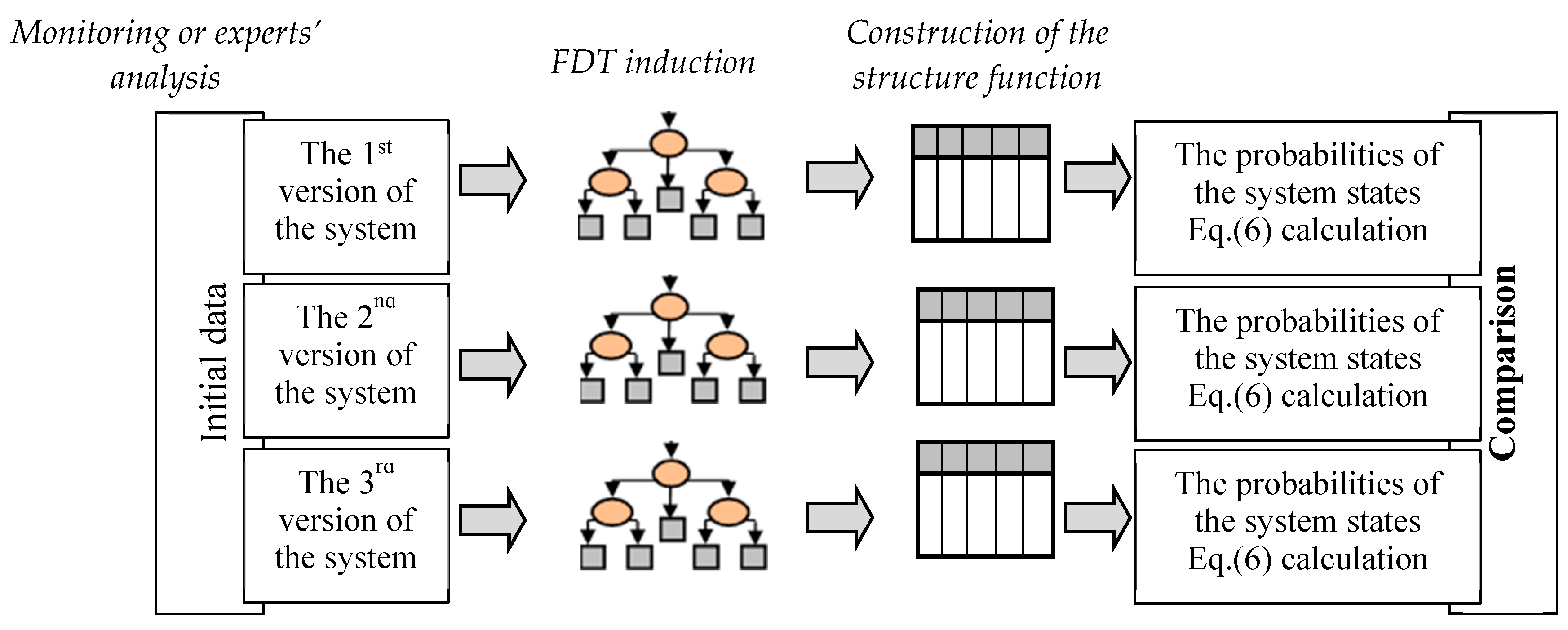
The procedure of the structure function construction can be considered a procedure of the decision table definition through the induction of the FDT based on uncertain data. According to this procedure, the essential steps of the proposed method for the structure function construction based on uncertain data are defined as (
Figure 1):
initial data preparation;
representation of the system model by the FDT; and
construction of the structure function based on the FDT.
The first of these steps is used to the transform of initial data into a form that is acceptable for FDT induction. As a rule, this is a table in which the known samples of input and output attributes are indicated. The second step is the induction of the FDT, which is considered in detail in
Section 5. The construction of the structure function is implemented during the third step according to rules by which the decision tree is transformed into the decision table. It is important to note that this method of constructing a structure function based on FDTs permits missing data to be computed (restored). Let us consider these steps for the construction of the structure function in more detail below.
4. Initial Data Preparation
The collection of data is implemented by monitoring a system or reviewing analyses of experts’ evaluations. The dataset is formed as a table of (
n + 1) columns (where
n is number of system components). The numbers in cells of the first
n columns represent component states and numbers in the last column are system performance levels. The
i-th column (
i = 1, …,
n) includes
mi sub-columns that indicate the
i-th component states from 0 to (
mi − 1) according to Equation (1). The last column has
M sub-columns as the number of the system performance levels. Rows of this table are formed by samples of monitored systems or experts’ evaluations. The cells include values of component states and system performance levels. The number values in cells range from 0 to 1. These values can be provided by interviews of experts or possibilistic fuzzy clustering [
63]. Per the first case, we have to take into account the differences in experts’ opinions of initial attributes. Therefore, all values of system performance levels and component states can be specified with a possibility ranging from 0 to 1. This range can be explained as the certainty degree of these values. If the value equals 1, then that expert’s certainty degree for this value is maximal (absolutely sure). These possibilities correspond to a membership function of the fuzzy data [
64]. Note that the sum of these possibilities for each value equals to 1. This demand for initial data representation is caused by the method of FDT induction.
We will interpret these values as fuzzy. A fuzzy set A with respect to a universe U is characterized by a membership function μA: U → [0,1], and an A-membership degree μA(u) is assigned to each element u in U. μA(u) gives us an estimation of u belonging to A. For u U, μA(u) = 1 means that μ is definitely a member of A and μA(u) = 0 means that μ is definitely not a member of A, while 0 < μA(u) < 1 means that μ is partially a member of A. If either μA(u) = 0 or μA(u) = 1 for all u U, A is a crisp set. A is fuzzy set in the opposite case. The cardinality measure of the fuzzy set A is defined by M(A) = ΣuU μA(u), which is the measure of the size of A.
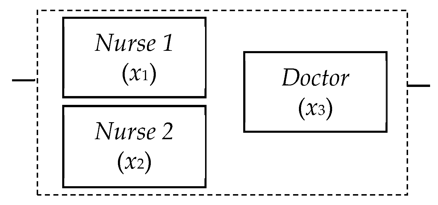
Let us consider the analysis of medical errors by a simple demonstration. In this example, a medical error system comprises the mistakes of two nurses and one doctor. The error estimation can be implemented as an analysis of the system of three components (
n = 3) (
Figure 2). Let us interpret this system in terms of MSS and introduce numbers of states for every component and number of the system performance levels. Let the system have three performance levels (
M = 3): 0—non-operational (the fatal medical error); 1—partially operational (some imperfection in patient care); and 2—fully operational (patient care without any complication). Two components
x1 and
x2 (that are interpreted as nursing mistakes) have only two possible states (
m1 =
m2 = 2): error (state 0) and absence of error (state 1). The doctor’s mistake can be modeled according to four levels (
m3 = 4) (i.e., from 0 (fatal error by the doctor) to 3 (doctor’s work is perfect)).
We have to find the dependence between mistakes of the nurses or doctor and the medical error in the system.
Table 3 shows expert’s evaluations of 12 situations, with each situation described by a separate row. In accordance with the first situation (the first row), it is determined that a mistake has occurred as a result of the first nurse (
x1 = 0) with a certainty of 0.9, and that no mistake has been made by this nurse (
x1 = 1) with a certainty of 0.1. The certainty of the second nurse having made a mistake is 1.0. Finally, the doctor’s work is determined to be perfect (
x3 = 3) with a certainty of 0.8, and to have included non-principal errors (
x3 = 2) with a certainty of 0.2. Similarly, the system performance (system medical error) is determined to have equaled 0 (non-operational, the fatal medical error) with a certainty degree of 0.3, or to have equaled 1 (partially operational, some imperfection in patient care) with a certainty degree of 0.7. We have interpreted all of these values according to the experts’ evaluations of possible values for input or target attributes. Note that the sum of these possibilities (certainties) for each value equals 1. The possibilities of the values permit data ambiguities to be specified. However, the information about investigated problems is not complete, as the data have not been obtained for all possible situations. To rectify this, the values of the input attributes and target attributes determined for the medical error analysis are defined by the membership functions in
Table 3. The sums of the membership degrees of attribute values are given in the bottom row of
Table 3.
The result of the first step is the table (dataset) that represents values of the system performance levels depending on the component states. This table doesn’t include all possible component states, and values of components states and system performance levels in this table are defined through terms of certainty (these values are not unambiguous exact values). The structure function definition (Equation (1)) separates all of the possible system states (samples) into M groups while taking into account the system components states. The problem of classifying uncertain and incomplete data is therefore solved by the application of a FDT.
5. FDT Induction for System Behavior Representation
There are different methods by which to induct an FDT [
33,
35,
64,
65]. These methods differ by the criteria of attribute selection in FDT induction. As shown in [
64,
65], the criteria of attribute selection are defined based on entropies. Two different conceptions of entropies for FDT induction have been considered and used in [
33,
35]. The entropy introduced by de Luka and Termini for fuzzy sets and Shannon probabilistic entropy is used for FDT induction in [
33]. The criteria based on the generalization of Shannon entropy as cumulative information estimation is applied for FDT induction in [
35]. The principal goal of these methods for FDT induction is to select splitting attributes and determine leaf nodes. An FDT is a structure that includes nodes, branches and leaves. Each node denotes a test on an initial attribute, each branch denotes the outcome of a test and each leaf represents a class label. The tree includes an analysis of input attributes in nodes and selections of values of the target (class) attributes in leaves. Each non-leaf node is associated with an attribute A
i A, or with a system component in terms of reliability analysis. The non-leaf node of the attribute A
i has
mi outgoing branches. The
s-th outgoing branch (
s = 0, …,
mi − 1) from the non-leaf node A
i agrees with the value
s of the
i-th component (
xi =
s). The path from the top node to the leaf indicates the vector state of the structure function by the values of attributes, and the value of the target attribute corresponds to the system performance level. If some attribute is absent in the path, then all possible values are possible for the associated system component. The target attribute value B
w agrees with one of the system performance levels and is defined as
M values ranging from 0 to
M − 1 (
w = 0, …,
M − 1).
The FDT induction is implemented according to the dependence between input n attributes A = {A1, ..., An} and a target attribute B. The construction of the system’s structure function supposes that the system’s performance level is the target attribute and that component states (state vectors) are input attributes. Each input attribute (component state) Ai (1 ≤ i ≤ n) is measured by a group of discrete values from 0 to mi − 1 that agree with the values of the i-th component states: {Ai,0, …, Ai,j, …, Ai,mi−1}. The FDT assumes that the initial set is classified as class values Bj of target attribute B.
For example, input attributes
A = {A
1, A
2, A
3} and target attribute B for the system in
Figure 2 are indicated in
Table 4 according to FDT terminology. Each attribute is defined as follows: A
1 = {A
1,0, A
1,1}, A
2 = {A
2,0, A
2,1}, A
3 = {A
3,0, A
3,1, A
3,2, A
3,3} and B = {B
0, B
1, B
2}. These attributes describe and structure the dataset in
Table 3.
The FDT algorithm used herein was initially proposed in [
33]. FDTs are inducted in a top-down, recursive divide-and-conquer manner. The algorithm can be briefly described as follows. Initial data are the training dataset (e.g.,
Table 3). We calculate the selection criterion for each attribute A
i not yet associated with nodes of the previous levels in this FDT branch. This criterion is based on the information’s estimation [
35]. We assign input attribute A
i with the maximum values of this selection criterion as the current node of the FDT. We analyze the obtained results for choice of leaves. If the branch is not finished as a leaf, we recursively repeat the process for this branch.
The information estimates used herein allow the criteria to induct an FDT with different properties [
35]. These estimates evaluate the dependence of the target attribute on input attributes in pieces. Cumulative mutual information
I (B;
,
) is an essential part of these criteria. This measure reflects how much information we obtain about target attribute B if we know the value of input attributes
and
. Conversely, the concept of entropy determines the measure of uncertainty for the value of the target attribute in cases where the corresponding values of the input attributes are known. These different cumulative information estimates permit the induction of an FDT with different properties. The algorithms for FDT induction and the criteria for building non-ordered, ordered or stable FDTs were originally proposed in [
62].
The selection criterion for splitting attributes
during induction of a non-ordered FDT is
where
are the values of input attributes
of the path from the root to node of the examined attribute
;
is the cumulative mutual information; and
is the cumulative conditional entropy of attribute
. Maximum value
iq in Equation (2) permits the selection of splitting attribute
. This attribute will be associated with a node of the FDT.
The cumulative mutual information between target attribute B, input attribute
and the sequence of attributes’ values
reflects an influence of attribute
on target attribute B when sequence
is known. In other words, cumulative mutual information is defined by part of the new information about target attribute B when a value of input attribute
is obtained. This measure is calculated as
where M(
) is the cardinality measure of fuzzy set
; and summands
,
,
and
are cumulative joint information. Let us have a sequence of
q − 1 input attributes
and target attribute B. The cumulative joint information of the sequence of values
(
q ≥ 2) and value B
j of target attribute B is [
35]
Other cumulative joint information , and are calculated analogously via Equation (4).
The splitting attribute for each level is selected from a set of attributes that are not used in the previous levels. Dividing cumulative mutual information in Equation (2) by the cumulative conditional entropy improves the problem of preferring attributes with a bigger domain of fuzzy terms. The cumulative entropy of input attribute
and sequences
is calculated by the next rule:
where M(
) is the cardinality measures of fuzzy sets
.
We will now describe the process of transforming a branch into terminal leaf. There are two tuning thresholds α and β in this method of FDT induction [
33,
35]. The first threshold α limits the frequency
f of the FDT branch. The frequency of the branch corresponds with the possibility of a situation described by the branch (i.e., possible combinations of certain values of input attributes
). This frequency equals
f(
) = M(
)/
N. The branch is finished as a leaf if the frequency of this branch is less than α.
Each branch of the FDT defines possible states of values Bj of the target attribute B. These states can be interpreted as certainty degrees for these values. A value with maximal certainty is recommended as the target attribute of this branch. The second threshold β limits FDT growth too. The FDT branch is finished as a leaf if the maximal certainty degree of this branch more than threshold β. Therefore, an FDT branch is finished as a leaf when the certainty degree of any value Bj of the target attribute is more than threshold β.
Thus, the criterion for finishing the FDT branch as a leaf occurs either when the frequency
f of the branch is below α, or when more than β percent of instances are left in the branch with the dominant value of the target attribute. These values are thus the key parameters that are needed to determine whether we have already arrived at a leaf node or whether the branch should be expanded further. Decreasing parameter α and increasing parameter β allows us to build large FDTs. On one hand, large FDTs describe datasets in more detail. On the other hand, these FDTs are very sensitive to noise in the dataset [
30]. We empirically select parameters α = 0.15 and β = 0.80. In practical applications, the optimal values of these parameters depend on the dataset and their values can be obtained experimentally. We estimate that a certainty degree of more than 0.80–0.90 would allow us to reach a sufficient decision. Moreover, the threshold frequency 0.10–0.15 eliminates the variants of no-principal situations. Notably, increasing the size of the FDT has no influence on the FDT root or the next FDT nodes, it merely adds new nodes and leaves to the bottom part of the FDT. These new nodes and leaves have a low bearing on decision-making. The considered algorithm for FDT induction is shown in
Figure 3.
Let us now explain the technique of FDT induction based on the monitoring data from
Table 1. We will build a non-ordered FDT with the parameters β = 0.80 and α = 0.15.
Preliminary analysis of the monitoring data shows that possible values of target attribute B are distributed as follows: value 0 has a certainty degree of 0.317 (3.8/12); value 1 has a certainty degree 0.425 (5.1/12); and value 2 has a with certainty degree of 0.258 (3.1/12) only. We have to compare the maximum of these values with threshold β. The value 0.425 is less than β = 0.80. Therefore, we have to build the first level of the FDT.
We show the cumulative information estimates based on one input attribute A3 only. This attribute has four possible values: A3,0, A3,1, A3,2 and A3,3. Similarly, target attribute B has three possible values: B0, B1 and B2.
The cumulative mutual information (Equations (3) and (4)) in target attribute B regarding attribute A3 equals
= I(B0; A3,0) + I(B0; A3,1) + I(B0; A3,2) + I(B0; A3,3) + I(B1; A3,0) + … + I(B2; A3,3) =
= 3.432 − 0.174 − 0.498 − 0.465 − 0.674 + 1.154 + 1.004 − 0.530 − 0.063 − 0.408 + 0.217 + 2.551 = 5.547,
where
I(B0; A3,0) = M(B0 × A3,0) × (−log2 M(B0) − log2 M(A3,0) + log2 M(B0 × A3,0) + log2 N) =
= 2.480 × (−1.926 − 1.585 + 1.310 + 3.585) = 3.432.
We have to calculate the cumulative entropies based on Equation (5):
We calculate all of the values
I(B; A
i) /
H(A
i) for each
i (
i = 1,…,4). The minimal value 5.547/23.995 corresponds to the input attribute A
3. Therefore, we assign attribute A
3 as a FDT root node (
Figure 4).
Let us explain this fragment of the first level of the FDT in more detail.
The attribute A3 has the maximum value of information estimation (Equation (2)). Therefore, this attribute is associated with the FDT root (top node). The data analysis starts with this attribute. This attribute can have the following possible values: A3,0, A3,1, A3,2 and A3,3. The value of attribute A3,0 stipulates target attribute B to be B0 (the system is non-operational) with a certainty degree of 0.827. The other variants B1 and B2 of target attribute B can be chosen with a certainty degree of 0.170 and 0.003, respectively. Frequency f for branch A3,0 is calculated as M(A3,0)/12. The result equals 3.0/12 = 0.250. This frequency f = 0.250 shows the possibility of an occurrence of values A3,0 when measuring the value of input attribute A3. The certainty degree of 0.827 for the value of B0 is more than β = 0.80; therefore, we stop the process of constructing the FDT for this branch.
If attribute A3 has other values (i.e., A3,1 or A3,2), then value B1 (the system is partially operational) of attribute B should be chosen with a certainty of 0.643 and 0.613, respectively. Similarly, for branch A3,3, the maximal value B2 (the system is fully operational) of attribute B should be chosen with a certainty degree of 0.655, respectively. These certainty degrees are below the priory threshold for the target attribute (β = 0.80). Moreover, the frequencies of occurrence for values A3,1, A3,2 and A3,3 (frequencies of FDT branches) are equal to f(A3,1) = 3.0/12 = 0.250, f(A3,2) = 3.1/12 = 0.258 and f(A3,3) = 2.9/12 = 0.242, respectively. The frequency of each branch is higher than the given threshold α = 0.15. Therefore, these branches do not finish as leaves.
Similarly, the process of inducting a non-ordered FDT is continued for the second and the third levels of the FDT. The final version of the non-ordered FDT is shown in
Figure 4.
In practical usage of this FDT, the values on each branch are fuzzy data A
i,j. Thus, the FDT can be represented by fuzzy decision rules [
66]. The FDT in
Figure 4 has eight leaves. We can formalize one fuzzy decision rule per each leaf. Of course, we have to use several fuzzy classification rules for analyses of new initial situations [
62]:
IF A3 is A3,0 THEN B is B0 with certainty 0.827;
IF A3 is A3,1 and A1 is A1,0 THEN B is B0 with certainty degree 0.616;
IF A3 is A3,1 and A1 is A1,1 THEN B is B1 with certainty degree 0.822;
IF A3 is A3,2 and A1 is A1,0 THEN B is B1 with certainty degree 0.672;
IF A3 is A3,2 and A1 is A1,1 and A2 is A2,0 THEN B is B1 with certainty degree 0.756;
IF A3 is A3,2 and A1 is A1,1 and A2 is A2,1 THEN B is B2 with certainty degree 0.651;
IF A3 is A3,3 and A2 is A2,0 THEN B is B1 with certainty degree 0.589; and
IF A3 is A3,3 and A2 is A2,1 THEN B is B2 with certainty degree 0.910.
So, we have transformed the initial data from
Table 1 into eight fuzzy decision rules. These rules are an essential part of an expert system, which describes decision-making based on this initial data. These fuzzy decision rules reflect the experts’ opinions in analyses of a medical error.
Comparisons of the proposed algorithm for FDT induction were implemented with other similar methods. This comparison was carried out with the machine learning benchmarks (dataset), each of which has the linguistic value of a class attribute [
67]. The theme of used datasets is applied to the medical area only. We divided each initial dataset into two parts—the first part (70% of the initial dataset) was used to build the structure function, while the second part (30% of the initial dataset) was used to verify the results. This process was repeated 1000 times, and average estimations were produced.
A fragment of the obtained results is shown in
Table 5. Columns labeled TS (total sets), NoA (number of attributes) and NoC (number of classes) describe initial dataset properties. The ratio columns give the number of errors for different approaches, which are calculated as the ratio of the number of incorrect structure functions to the total number of inducted structure functions. The results are recorded in the columns labeled FDT, ysFDT, C4.5, CART, nBayes and
kNN, which refer to our proposed algorithm of FDT induction [
35], FDT building algorithms [
33], algorithm C45, CART, naïve Bayes classification and
k-nearest neighbors, respectively. The best results are written in a bold font. We have indicated several variants as the best choice if the difference between them was below 0.005 (less than 0.5%). The experimental results demonstrate our approach’s rank compared with the other methods.
The full classification accuracy for algorithm C4.5, CART, naïve Bayes classification,
k-nearest neighbors, and so on are compared in [
68] for different datasets. The obtained results confirm the efficiency of our approach.
6. Construction of the Structure Function Based on the FDT
FDT is a classification structure that permits the separation of instances (in this case, the state of the system equals the value of the structure function) depending on input attributes (that agree with component states equaling the values of the structure function variables). FDT permits the investigation of all possible values of the structure function if the combinations of the values of its variables are defined as input attributes. The structure function is formed as a decision table that classifies the system performance level for each possible profile of component states.
Let us construct a structure function of the system for medical error analysis by the FDT (
Figure 4) inducted based on monitoring data from
Table 1. The structure function of this system agrees with the decision table for the FDT that is formed from all of the input attributes. Therefore, all possible values of the component states from
x = (0 0 0) to
x = (1 1 3) must be classified into
M classes of the system performance levels.
For example, assume that the state vector is
x = (0 0 0). Analysis based on the FDT starts with the attribute A
3 (
Figure 4) that is associated with the third component. The value of this component state is 0 (
x3 = 0) for the specified state vector. Therefore, the branch for the attribute value A
3,0 is considered. The branch of this value has a leaf node, therefore the target attribute value at this node is defined as B
0 and analysis of other attributes is not necessary in this case. The system performance level for this state vector
x = (0 0 0) is 0 (the system is non-operational; fatal medical error) with a certainty degree of 0.827.
Let us consider a state vector in which x = (1 0 1). We analyze attribute A3, and the value of this attribute is A3,1 for this state vector. According to the FDT, the branch with attribute value A3,1 is selected. Next, attribute A1 is analyzed in a similar manner. The estimation of this attribute is implemented using a branch with an attribute value A1,1 because the specified state vector includes x1 = 1. The branch of this value has a leaf node; therefore, the target attribute can take any of the following possible values: value 0 (with a certainty degree of 0.006), value 1 (with a certainty degree of 0.822) and value 2 (with a certainty degree of 0.112). The value of the target attribute should be defined as the value with the maximal certainty degree, so the system performance level for the specified state vector is φ(x) = 1 with a certainty of 0.822.
Analysis of other state vectors is similar and allows all possible values of the system performance level to be obtained in the form of the structure function defined in
Table 6—the certainty degree of the structure function values for each state vector appears in the bottom row.
The missing monitoring data can be restored based on FDTs. An interesting outcome from the table is that in cases of component vector x = (0 1 1), the system state is 0, while for x = (1 0 1), the system state is 1. Thus, it seems that in the event of one type of doctor error, the two nurses have different influences on the system. This outcome is inferred from the initial data. Each of the nurses has their own experiences, different qualifications and unique mistakes. Our algorithm can trace such influences, which was not obvious at the start.
7. System Evaluation Based on the Structure Function
The representation of the system using the structure function allows different indices and measures to estimate system reliability. One of the basic indices is system probability of system performance level
Aj [
17]:
where
j = 0, …,
M − 1 and
j = 0
A0 is system unavailability:
U =
A0;
is the probabilities of the
i-th component state
si, which represents the initial data for the system evaluation and is based on the structure function (
si = 0, …,
mi − 1):
Therefore, probabilities of system performance can be calculated according to the typical methods used in reliability engineering based on the structure function. Other measures can also be computed by the structure function; for example, the sensitivity analysis algorithms from [
17,
69,
70] measuring system reliability can be used for the similar analysis of medical errors based on the structure function.
Let us consider an example in which the structure function is applied in the HRA of a healthcare system. According to the request of this investigation, complications in the familiarization and exploitation of new devices is analyzed and evaluated.
This investigation was provided for neonatal jaundice (or neonatal hyperbilirubinemia) examination in the neonatology department. Doctors and nurses were involved in the diagnosis as a rule. A jaundice meter was introduced as a new device for providing a diagnosis. The result of this device’s exploitation was investigated during the first two months of exploitation and after one year of exploitation.
Three versions of the system were analyzed to investigate the influence of this device on a diagnosis.: (1) a check-up implemented by the doctor and nurse only; (2) the doctor and nurse examine a patient and use the new device (i.e., the jaundice meter), which is exploited for two months only; and (3) the device is used for one year and the medical staff (doctor and nurse) have experience with its exploitation. The third component (device) was included in the second and third versions of the system.
Each proposed version of the system was considered in order to construct a structure function through the FDT for each of them (
Figure 5). The interpretation of this system in terms of FDT induction is presented in
Table 7. The initial data used to create a repository for each of the system’s versions was collected from the monitoring of patient examinations and structured interviews with experts (
Table 8). Five experts, two doctors and three nurses were involved in the investigations. All evaluations were implemented using possibilities of every component value and system performance level; experts introduced all values as a number from 0 to 1. For example, the experts evaluated a doctor’s work as perfect with a possibility of 0.9, and incorrect with a possibility of 0.1; the nurse’s work as perfect with a possibility of 0.4, and as incorrect with a possibility of 0.6; and the device as functioning with a possibility of 1, “fully operational“ with a possibility of 0.8 and “partially operational” with a possibility of 0.2. After pre-processing analysis, the initial data were transformed into three repositories. However, some of the situations were not obtained by the experts’ evaluations. Therefore, these repositories represented uncertain and incompletely specified data.
The system state probabilities (Equation (6)) were calculated and compared for all versions of the system. The probabilities of the component states (Equation (7)) were introduced as initial data. We evaluated this sensitivity of this system based on the structural importance measures of the system components calculated with the application of the Direct Partial Logical Derivatives for the structure function. The definition and algorithm for calculating these measures are considered in detail in [
70]. The structural importance measure reflects the changes of probability in the specified system states depending on the specified changes of the components.
The first system’s version was considered to be a system of two components, while the second and third versions included three components (two human components and one technical). Three performance levels were introduced for each of the system versions (
M = 3). Two human components with three states (
m1 =
m2 = 3) were considered for all versions:
x1 = the work of the nurse and
x2 = the work of the doctor. Device states (the third component
x3) had only two states (
m3 = 2): error and functioning. The structure function for each system versions was formed using FDTs that were inducted based on data collected in the repositories. The constructed structure functions for three versions of the system are described in
Table 9.
First of all, the probabilities of the system performance levels were computed according to Equation (6), as shown in
Figure 6. The diagram in
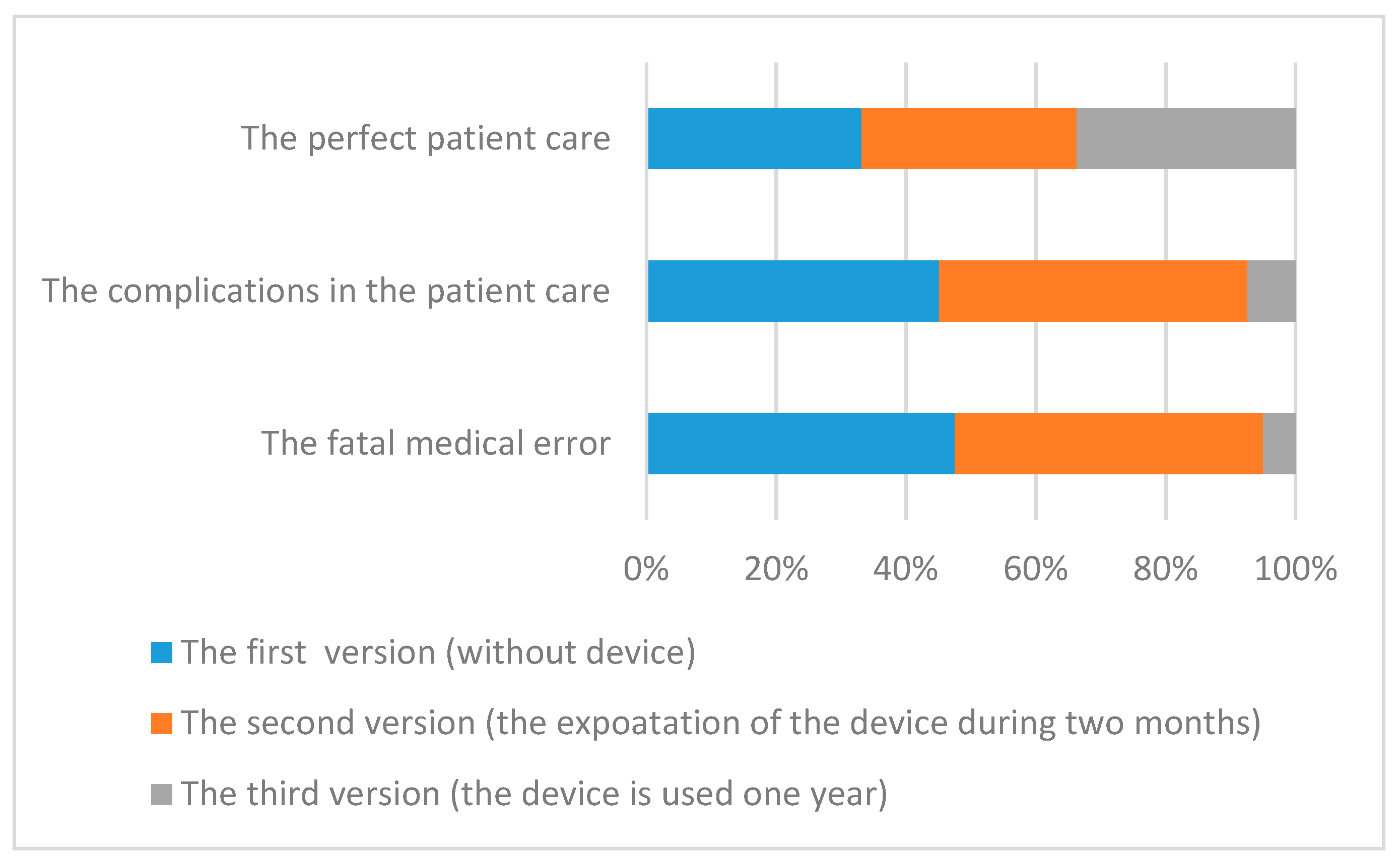
Figure 6 shows the probabilities of the system performance levels on the y axis for three version of the system. According to these diagrams, application of the device did not have a good influence on patient care during the first two months. The error number (bottom diagram) did not change; the number of the complications (middle diagram) slightly increased (the difference of these probabilities is 0.0008) and the number of perfect cases (top diagram) decreased. The application of the device in the first two months caused an insignificant decrease in the amount of perfect patient care. The probability of perfect cases for the second system version was less, at 0.0008. The number of medical errors did not increase within two months of using a jaundice meter, which is a good result. The essential influence of the new device’s application on patient care was discovered after one year—the number of medical errors decreased and the number of perfect cases of patient care increased. The probability of perfect cases of patient care increase was 0.01, and probability of medical error decreased to 0.001. The proportional changes of these probabilities are illustrated in diagram in
Figure 7. The fatal medical errors for the first version of the system had maximal proportion in comparison with the two other versions of this system. Therefore, the usage of new devices had a positive influence on the reduction of medical errors in the considered system. The accuracy of these results was the result of the FDT induction discussed in
Section 5 for different datasets according to the ratio of the number of incorrect values for the constructed structure function.
The sensitivity of this system calculated according to the algorithm in [
70] depended on the mistakes of the doctor or nurse, and the failure of the device is shown in
Figure 8, with the doctor’s mistake being most important of all versions. As a result, the factors causing the doctor’s mistakes are important and have been additionally investigated.
A doctor’s mistakes can occur due to general conditions (haste, poor work environment, poor surroundings, incorrect communication with patient attendant) and specifics related to the device used (e.g., screen color, illuminance, etc.). These causes have been further investigated in a similar manner to the application of the construction of the structure function. This investigation showed a high influence of special causes on the doctor’s mistakes, with haste being the most significant of the general causes according to the provided analysis. Therefore, ensuring sufficient time for patient examination is a necessary condition for decreasing medical errors during examination.


