Article

Machine Learning Algorithms for Smart Data Analysis in Internet of Things Environment: Taxonomies and Research Trends

by
Mohammed H. Alsharif
1,*,
Anabi Hilary Kelechi
2,
Khalid Yahya
3 and
Shehzad Ashraf Chaudhry
4
1
Department of Electrical Engineering, College of Electronics and Information Engineering, Sejong University, 209 Neungdong-ro, Gwangjin-gu, Seoul 05006, Korea
2
Department of Electrical Engineering and Information Engineering, College of Engineering, Covenant University, Canaanland, Ota P.M.B 1023, Ogun State, Nigeria
3
Department of Electrical and Electronics Engineering, Faculty of Engineering and Architecture, Istanbul Gelisim University, Avcılar, 34310 İstanbul, Turkey
4
Department of Computer Engineering, Faculty of Engineering and Architecture, Istanbul Gelisim University, Avcılar, 34310 İstanbul, Turkey
*
Author to whom correspondence should be addressed.
Symmetry 2020, 12(1), 88; https://doi.org/10.3390/sym12010088
Submission received: 10 December 2019 / Revised: 26 December 2019 / Accepted: 30 December 2019 / Published: 2 January 2020

Abstract

:
Machine learning techniques will contribution towards making Internet of Things (IoT) symmetric applications among the most significant sources of new data in the future. In this context, network systems are endowed with the capacity to access varieties of experimental symmetric data across a plethora of network devices, study the data information, obtain knowledge, and make informed decisions based on the dataset at its disposal. This study is limited to supervised and unsupervised machine learning (ML) techniques, regarded as the bedrock of the IoT smart data analysis. This study includes reviews and discussions of substantial issues related to supervised and unsupervised machine learning techniques, highlighting the advantages and limitations of each algorithm, and discusses the research trends and recommendations for further study.

1. Introduction

With the current inclination towards “smart technology”, data are being generated in symmetric large quantum, resulting in the concept of big data. Big data can be defined based on the “Five V’s”: high-velocity, high-volume, high-value, high-variety, and high-veracity. To fully exploit the usefulness of big data, there should be an astute, cost-effective, and innovative technique for extracting and processing raw data, thus leading to greater insight, problem-solving, and process automation [1]. The Internet of Things (IoT) has the capacity to generate novel datasets. Simply by mimicking such various human sensory attributes as vision, hearing, and thinking, a machine can communicate to another machine, exchange important information codes, and execute instantaneous decisions with little human assistance [2]. The system must access experimental unprocessed data, originating from diverse media within a network, study the data, and obtain useful information. Machine learning (ML) technology is a specific type of algorithm that can be applied to many different domains, symmetric data types, and symmetric data models [3]. Accordingly, ML is seen as providing a significant platform towards achieving smart IoT applications [4].
ML is a type of artificial intelligence (AI) that provides machines with the ability to learn pattern recognition [5]. In the absence of a learning algorithm, ML cannot be complete because it functions as an input source for the model to understand the underlying attributes of the data structure. In the literature, the learning algorithm is often referred to as a training set or training model. Thus, learning algorithms are technically grouped into three main categories of learning (Figure 1) [6]:
  • Supervised learning. This learning algorithm uses samples of input vectors as their target vectors. The target vectors are typically referred to as labels. Supervised learning algorithm’s goal is to estimate the output vector for a specific input vector using learning algorithms. User-cases that have target identifiers are contained in a finite distinct group. This is typically referred to as classification assignment. When these targeted identifiers consists of one or more constant variables, they are called regression assignment [5].
  • Unsupervised learning. This learning algorithm does not require labeling of the training set. The objective of this type of learning is to identify hidden patterns of the analogous samples in the input data. This is commonly called clustering. This learning algorithm provides suitable internal understanding of the input-source information, by preprocessing the baseline input-source, making it possible to reposition it into a different variable space of the algorithm. The preprocessing phase enhances the outcome of a successive ML algorithm. This is typically referred to as a feature extraction [7].
  • Reinforcement learning. This learning algorithm involves deploying similar actions or series of actions when confronted with same problem with the aim of maximizing payoff [8]. Any outcome that does not lead to favorable expectation is dropped and conversely. Expectedly, this type of algorithm consumes lots of memory space and is predisposed in applications that are executed continuously.
This study will focus on supervised and unsupervised learning, as both are considered the main pillars of the IoT smart data analysis [5]. Since, there are numerous algorithms in ML technology, assisting IoT big data analysts in choosing the appropriate and suitable algorithm will enhance their understanding of the topic as well as reduce their project execution completion time. The key contributions of this study are the presentation of a comprehensive analysis of the related literature on supervised and unsupervised machine learning techniques considered as the main pillars of the IoT smart data analysis. These techniques are investigated based on their respective sub-domains, as well as advantages and limitations to achieving a precise, concrete, and concise conclusion. This article also addresses current research trends in IoT smart data, open issues being pursued in this area.
The rest of this chapter is organized as follows. Section 2 discusses taxonomies of supervised and unsupervised machine learning techniques based on their respective sub-domains with their advantages and limitations. Section 3 reviews the research trends and open issues. Section 4 elaborates the conclusions and recommendations.

2. Taxonomies of Supervised and Unsupervised ML Algorithms

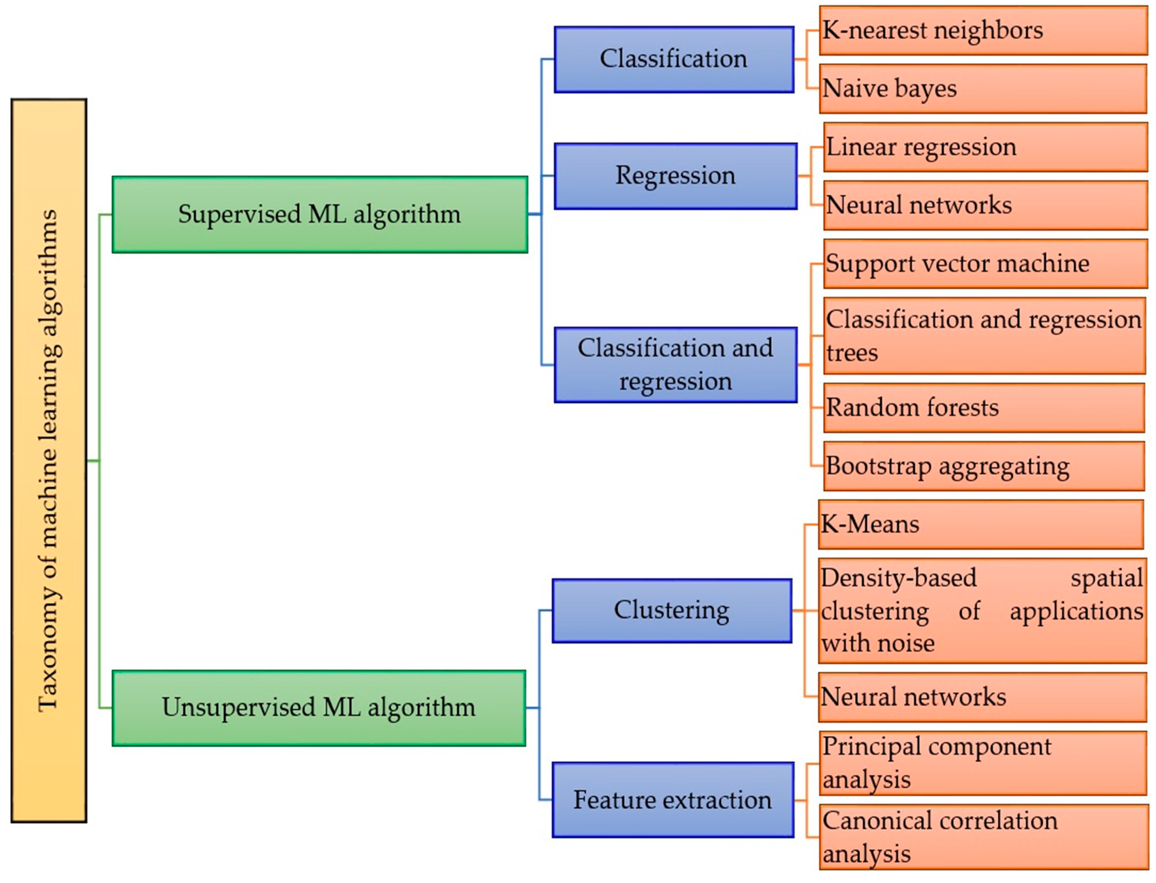
The majority of practical ML uses supervised learning. Supervised learning is a process of learning an algorithm from the training dataset where the input variables and output variables are available. An algorithm is used to learn the mapping function from the input to the output. The aim is to approximate the mapping function so that when we have new input data, we can predict the output variables for that data. Supervised learning problems can be further grouped into regression and classification problems [9]. Unsupervised learning is where you only have input data and no corresponding output variables. Unsupervised learning problems can be further grouped into clustering and feature extraction problems [10]. The summarized taxonomy of supervised and unsupervised machine learning algorithms is given in Figure 2. In addition, Table 1 provides a summarized comparison of the basis and notable attributes, as well as advantages and limitations for each algorithm of the sub-domains of a supervised and unsupervised ML. In the following subsections, a detailed discussion is presented.

2.1. Supervised ML Algorithm

Most practical ML deploys supervised learning. In supervised learning, the available datasets are called “true” datasets or “correct” datasets. The algorithm is “trained” by using these input datasets. This is referred to as: training data. During this procedure, the algorithm roles reduces to making estimations on the given input experimental data and expanding or contracting its evaluations based on the “ground truth” as baseline, repeating the process until the algorithm achieves some degree of accuracy universally acceptable [11]. An ML algorithm will, typically, adjust and satisfies a cost function. A cost function quantifies the error between the “ground truth” and algorithm calculations. Minimizing the cost function, allows for training the model to yield results that align to more precise values (ground truth). Minimizing cost function can be achieved with the utilization of a gradient descent technique [12]. Different gradient descent techniques such as stochastic gradient descent, momentum-based gradient descent, and Nesterov accelerated gradient descent [13] have been applied to ML training paradigms. In an example where ‘m’ represents the number of trainings, each training can be denoted in a pair, as follows: (x, y). In this example the x can signify the input experimental data and y signifies the class identifier label. The input experimental data x represents an n dimensional, while individual dimension links to an explicit feature or a specific variable. In this example, the ML algorithm is aligned with a specific sensor system embedded in the program to accommodate the IoT application. [14]. Supervised learning problems can be further grouped into classification and regression problems [12]. In the following subsections, a detailed discussion is presented.

2.1.1. Classification Tasks

Classification is a technique to categorize the data into a desired and distinct number of classes where a label is assigned to each class [15]. There are many methods to classify the data, a detailed discussion about the types of classification algorithms is given in the following subsections.

K-Nearest Neighbors (KNN)

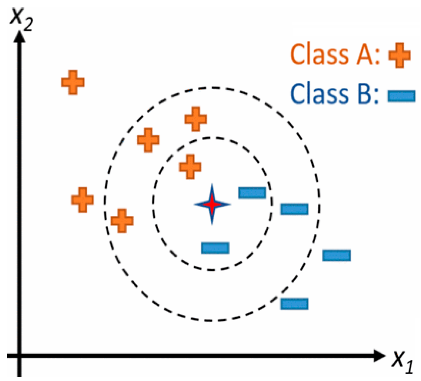
The k-nearest neighbors (KNN) algorithm is a supervised ML algorithm that can be used to solve both classification and regression problems. However, it is more widely used in classification problems [16]. There are three important aspects that are used to evaluate any algorithm, namely (i) ease to interpret output, (ii) calculation time, and (iii) predictive power. KNN is simple, easy to implement, and commonly used because its ease of interpretation and low calculation time. In classification and regression problems, the input dataset comprises of k that is nearest to the training datasets deployed in the featured set. The output is dependent if KNN is deployed to function as classification or regression algorithm: (i) In the case of KNN classification, the ensuing result is a subject to a class membership function [5]. To classify an object, a range of voting is executed by its neighbors. At the end of the voting, the object is allocated to the class most prominent amongst its k nearest neighborhood (k is supposedly a non-negative integer). On the occasion that, k = 1, the object is mapped to the class of its single nearest neighborhood. (ii) For KNN regression, the ensuing result is the characteristic value for the object which is the mean figure of k’s nearest neighbors. To locate the k of a data point, Euclidean distance, L norm, angle, Mahalanobis distance, or Hamming distance can be used as the distance metric [17,18]. A KNN model is shown in Figure 3, for k = 3, imagine that in this example, the test point (star) belonging to class B and for k = 6, the point is classified as belonging to class A. In this example, KNN is a non-probabilistic and non-parametric model [19]. It is common for this to be the first choice for a classification study when no prior knowledge of the data distribution is available. In this illustration, KNN supplies all labelled input points. So, the question is raised what should be done with the unknown sample or samples? Resolving this dilemma can lead to significant computational expense. Classification of this type is based on a distance metric referred to as a similarity measure. Any sample labeled as unknown must be then classified by majority vote of its k nearest neighbors. Because complexity intensifies as the dimensionality goes up, dimensionality decrease approach [20] becomes crucial prerequisite before deploying KNN. This is necessary to circumvent effects that might eschew dimensionality. For example, KNN classifiers are used for stress detection in the monitoring of human physiological signals [21] as well as in the detection of seizure activity in a patient with epilepsy [22].
With Figure 3 as our example, the problem can be formulated as; thus, let x connotes input dataset (data point), while, its K nearest neighbors are denoted with Nk (x). Then, the estimated class label identifier for x can be denoted as y, with the class variable using unassigned variable t. In addition, 1 (.) can indicate the attribute: 1 (s) = 1 if s is true and 1 (s) = 0 conversely. By way of compact notation, the above classification assignment is depicted as [5]:
p ( t   =   c | x , K )   =   1 K i N k ( x ) 1 ( t i   =   c ) y   =   max c p ( t   =   c | x ,   K )    
Despite the benefits that can be achieved with this algorithm, (such as no training period) which allows for new data to be added seamlessly without negative impact on the accuracy of the algorithm; one major KNN shortcoming is requirement of large storage memory to store the whole training set data. This unique attribute has reduced the acceptability of KNN in the face of high dimensional datasets because of the increasing dimension cardinality, thus making it increasingly difficult for the algorithm to calculate the norm between the dimensions. In addition, the KNN is sensitive to noise in the dataset [23]. We need to manually input missing values and remove outliers. The authors in [24] have addressed incident of large data sets via designing of a tree-based search with a one-off computation. Additionally, the authors in [25] suggest a structure for learning multiple metric combinations utilizing a vigorous and unique KNN classifier. Other authors [26] link KNN with a rough-set-based algorithm that has been used for classifying travel pattern regularities.
Several improvement variants of the conventional KNN algorithm exists, typical the wavelet based KNN partial distance search (WKPDS) algorithm [27], equal-average equal-norm nearest neighbor code word search (EENNS) algorithm, and the equal-average equal-variance equal-norm nearest neighbor search (EEENNS) algorithm [28].

Naive Bayes

A naive Bayes classifier is one of the numerous supervised machine-learning algorithms with underlying principle derived from the Bayes’ Theorem, which assumes that data attributes are statistically uncorrelated. Presented with a novel, unverified data point (input vector) x = (x1, …, xM), the task reduces to finding an algorithm that estimates the expected outcome with some level of accuracy. In this regards, a naive Bayes classifiers assumes a model of choice. Naïve Bayes is a subset of probabilistic classifiers which is motivated by Bayes’ theorem with the underlying “naive” postulation of independence between the structures of x assumes the class variable t. The fundamental principle of this theorem is based on the naive assumption that input variables are statistically uncorrelated from one another, i.e., the likelihood of inferring more information about other variables in the presence of additional variable is slim. Using Bayes’ theorem, the form can be expressed as follows [29]:
p ( t   =   c | x 1 ,   , x M )   =   p ( x 1 ,   ,   x M | t   =   c ) p ( t   =   c ) p ( x 1 ,   ,   x M )
Invoking the naive independence model concept and after some simplifications, the result is:
p ( t   =   c | x 1 ,   , x M ) p ( t   =   c ) j   =   1 M p ( x j | t   =   c )
The form of the classification task can be expressed as follows [30]:
y   =   max c p ( t   =   c )   j   =   1 M p ( x j | t   =   c )
where y connotes the estimated class identifier for x. Various naive Bayes classifiers adopts various schemes and distributions to forecast p (t = c) and p (xj|t = c).
The naive bayes classifier requires fewer datasets for training, and is equipped to overcome the curse of data points high-dimensionality while being robust and highly scalable [31]. Additionally, the Naive bayes classifier is the model of choice for several user-cases of spam filtering [32], text categorization, and automatic medical diagnosis [33]. On the other hand, the authors in [34] utilized this algorithm to aggregate features for evaluating trust value and calculating the last numerical trust value of the farm produce. Despite the benefits that can be achieved by this classifier, the main limitations of this classifier (Naive Bayes) are the assumption of independent predictors and assumption that all the attributes are mutually independent. However, in real life, it is almost impossible that we get a set of predictors which are completely independent [30]. Conversely, if the categorical variable has a category in the test data set, that are not visible in the training data set, then the model will assign a 0 (zero) probability and thus, not useful to making estimate. In the literature, this phenomenon is referred to as zero frequency. However, to overcome this issue, smoothing technique is often deployed. The most common smoothing approach is the Laplacian estimation [35].

2.1.2. Regression Tasks

Regression models are used to predict a continuous value. A detailed explanation of the different types of regression tasks, with some important concepts are presented in following subsection.

Linear Regression

Linear regression is a ML algorithm motivated by supervised learning and specifically designed to implement regression task. Regression models aim to provide a prediction value based on independent variables. It is prominent in understanding the relationship between variables and estimating possible results [36]. The most salient point in regression models is the relationship existing dependent and independent variables. The objective of linear regression is to learn a specific function f(x, w). In this case, one would plot the following: f: ϕ(x) → y. This is the linear amalgamation of a set of fixed linear or nonlinear functions from the input variable. This can be symbolized as the basic function: ϕi(x) [29].
f(x,w) = ϕ(x)Tw
where w signifies the weight vector (i.e., matrix), the equation would be conveyed as w = (w1, …, wD)T, and ϕ = ( ϕ1, …, ϕD)T. A broad range of basic functions exist to assist in creating this application. For example: polynomial, gaussian, radial, or sigmoidal basic functions could be used in this application [37].
A key concern is training the model for application. Several approaches are available: ordinary least square, regularized least squares, least-mean-squares (LMS) and Bayesian linear regression. The LMS approach is very useful because it is quick, can easily be adapted to accommodate large data sets, and can learn the parameter requirements over the internet by using stochastic gradient descent (sequential gradient descent) [38]. Using the appropriate basic function, random nonlinearities in the mapping from input variable to output variable can be identified. However, the use of fixed basis functions can lead to significant shortcomings (e.g., an upsurge in input space dimensionality leads to a precipitous increase in the cardinality of the fundamental functions) [39]. Linear regression algorithms have a high execution rate [40]. For example, this algorithm is adept for analyzing and predicting buildings energy usage.
In contrast, neural networks are effective in addressing certain fundamental functional issues as well permitting the model to acquire the system parameters of the fundamental functionality. In addition, neural networks have high computational capability in the face of novel data, due to its compact nature. Additionally, they are properly tuned to solve regression and classification tasks. Though, this comes with expense of large amount of experimental training data to train and learn the model [41]. In the literature, the exposition of various types neural networks, utilizing various architectures, use cases, and applications are common.

2.1.3. Combining Classification and Regression Tasks

Support Vector Machine (SVM)

Classical support vector machine (SVM) is a support-vector network that can be utilized with supervised learning models. This model is a non-probabilistic, binary classifier that can be used to identify the hyperplane that divides classes of the training set. This provides a maximized margin. The predicted label of a previously unobserved data point can be determined by the side of the hyperplane on which it falls [42]. The major attraction of SWM is that with a few training points, a high degree of accuracy is ensured. These training points are support vectors that can categorize any novel data point in the network. SVMs not only perform binary classification, they are also able to do multiclass classification. Four such models are: all-vs-all (AVA) SVM, one-vs-all (OVA) SVM, structured SVM [43], and the Weston and Watkins version [44]. Besides linear classification, SVMs can perform non-linear classification. This can be useful for finding the hyperplane of a non-linear functioning input variable. For example, an input variable can be mapped into a high-dimensional feature space. This process is referred to as a kernel trick [45]. To design this task, identify the typical vector of the hyperplane as w and the parameter for controlling the offset of the hyperplane as b. To safeguard that SVM will be able to control for outliers in the data, a variable ε i can be introduced for every training point xi. This is a slack variable that determines the distance that the training point encroached upon the margin in units of |w|. In this example, a binary linear classification task can be designated as a constrained optimization problem in the following manner [46]:
min w ,   b , ε f ( w , b , ε )   =   1 2 w T w   +   C i   =   1 n ε i Subject   to   y i ( w T x i   +   b )     1   +   ε i     0   i =   1 ,     n ;   ε i     0
where parameter C > 0 determines how heavily a violation is punished. Furthermore, the parameter C is a hyperparameter whose choice are implemented either from cross-validation or Bayesian optimization. There exist various strategies to address the constrained optimization problem in Equation (6). P-pack SVM [47], quadratic programming optimization [48], and sequential minimal optimization [49] are techniques that can be applied to this problem. SVM is an excellent supervised learning model that can efficiently address high dimensional data sets. It is particularly effective for addressing memory usage because it utilizes support vectors to facilitate prediction. However, this model has a significant drawback in that it lacks technique to directly stipulate probability estimates. SVM is very suitable in numerous practical applications including hand-written identification problem [50], image recognition [51], and protein arrangement [52]. Finally, it is possible to train SVMs in an online fashion as discussed in [53]. The authors in [54] suggested a technique using Intel Lab Dataset; data set composed of four basic environmental attributes of (temperature, voltage, humidity and light) obtained via S4 Mica2Dot sensors. The authors in [55] applied SVM to classify traffic data.

Classification and Regression Trees (CART)

Classification and regression trees (CART) is a fast training algorithm that has found applicability in classifying smart citizen behaviors [56]. Though some of the already discussed algorithms are deployed in modelling machine learning, decision trees are unique. In the family of the classical decision tree and its variant algorithms, random forest is among the popular approaches in use. In the CART algorithm, the input domain is divided into bloc-aligned cuboid sections Rk, and then a distinct classification or regression scheme is applied to each section to estimate the character of the data points located in that section [57]. Presented with a novel, untested input experimental vector (data point) x, the goal of estimating the appropriate target attribute could be described as binary tree mechanism which corresponds to a successive decision-making approach. The primary purpose of a classification algorithm is to predict a specific attribute for a given bloc. Meanwhile, the regression algorithm focusses on predicting a constant for each bloc. Mathematically, the classification task is formulated to recognize an attribute variable using a non-continuous random variable t and the estimated attribute identifier for x by y. The classification task is denoted as follows [29],
p ( t   =   c | k )   =   1 | R k | i R k 1 ( t i   =   c ) y   =   max c p ( t   =   c | x )   =   max c p ( t   =   c | k )
Equation (7) connotes that it will be tagged by the most significant mode in its appropriate bloc [29].
Similarly, to model the regression task, let y represent the output vector by a number, t and the estimated output vector for x by y. Then, the regression task is stated as,
y   =   1 | R k | i R k t i .
The output vector for x is the average of the output vectors of data set in a specific region.
For CART training, the tree topology should be derived using the training set. This implies obtaining the fragmented property at individual point, together with the limiting parameter figure. Locating an ideal tree topology is an NP-complete problem. In the literature, this is known as a greedy heuristic, which fashions the tree in a top-down approach and chooses the optimal fragmented point by point to train CART. The problem of overfilling and attaining better generalization, requires that some stopping criteria is necessary for the tree design. Some of the potential terminating benchmark are; the highest depth attained, if the branch distribution is unadulterated, if the gains of separation is lower than a certain benchmark, and if the cardinality of samples in every single branch is lower than the criteria benchmark. Additionally, the pruning technique is effective in dealing with the problem of overfitting [56,58]. The main advantage of CART is that it is rapid and adjustable to big data sets. Unfortunately, it is responsive to the training set selected [59]. A significant drawback of this technique lies in the unsmooth identification of the input domain since each bloc of the input domain is related with a unique identifier [9].

Random Forests

Random forests or random decision forests are an ensemble learning method for classification, regression and other tasks that operate by constructing a multitude of decision trees at training time and outputting the class that is the mode of the classes (classification) or mean prediction (regression) of the individual trees. In random forests, instead of training a single tree, an army of trees are trained. Each tree is trained on a subset of the training set, chosen randomly along with a replacement, using a randomly chosen subset of M input variables (features) [60]. There are two situations for estimating the attribute of a novel, unexplored data point: (1) in classification tasks, is tuned as the highest occurring identifiers predicted by each tree; (2) in regression tasks it is tuned as the average of the estimated identifier by individual tree. A balance exists between various figures of M. A figure of M that is insignificant results in arbitrary trees with low estimation capability, while a bogus figure of M might result to very familiar arbitrary trees.
Random forests are noted to be extremely accurate. Nevertheless, this is at the expense of meaningful human interpretability [61]. However, they are agile and dynamic for big data sets and have many practical usages, typically including body pose recognition [62] and body part classification.

Bootstrap Aggregating

Bootstrap aggregating, often referred to as bagging, is a collaborative technique whose goal is to enhance and improve the precision as well as the robustness of ML algorithms, resulting in a decrease of overfitting issues. Using this approach, K novel M sized training datasets are arbitrarily selected from the raw dataset with substitutions. Consequently, the newly selected data training set are trained using a ML model [63]. The estimated identifier of a novel, untrained data point is denoted to be the mode of the identifiers estimated by individual scheme in classification assignment and is denoted to be the average of regression assignments. By using different ML schemes such as CART and neural networks, their bagging schemes enhance results. Although, bagging deteriorates the operation of robust models e.g., KNN. Typically, real-life usage scenarios include customer attrition prediction and preimage learning [29].

2.2. Unsupervised ML Algorithm

Unsupervised ML algorithms decode data morphology from a dataset without reference to already identified results. Different from supervised machine learning, unsupervised machine learning methods are not ideal for regression and classification task based on the fact there is opaqueness of the expected outcome. Hence, it is difficult to train the model Unsupervised learning finds applicability in decoding the data fundamental structure. Of all the different types of unsupervised algorithm, clustering is the most widely used. A detailed discussion about the types of the unsupervised machine learning algorithms is given in the following subsections.

2.2.1. Clustering

K-Means

The modus operandi of K-means algorithm lies towards grouping unidentified data set into K clusters or constellations. Simply by arranging datasets with same property into one cluster and otherwise. Using the traditional K-means model, the norm between datasets denotes the degree of resemblance. Hence, K-means sets out to discover K cluster centers, represented as [s1, …, sk], with the norm between datasets and their closest center being reduced [54]. Grouping data points into clusters centers can be implemented via a set of binary indicator variables πnk [0,1]. On the occasion that the data point xn is designated to the cluster center sk, then πnk = 1. This can be modelled thus:
min s , π n   =   1 N k   =   1 k π n k | | x n     s k | | 2 Subject   to   k   =   1 K π n k   =   1 ,    n =   1 ,   ,   N
K-means is a highly efficient and flexible algorithm with fast convergency rate. Note, an online stochastic version of K-means exists along the with the offline version [62]. References [50,52] analyzed a strategy to deploy the K-means algorithm towards smart city and smart home data management with impressive outcomes. Unfortunately, this technique is confronted with numerous setbacks due to the deployment of the Euclidean norm as a measure of comparison. Typically, the limitations arose because of the categories of data variables being used, and cluster centers are unstable against datapoint located outside the main region. Furthermore, the K-means model designates individual data point uniquely to a cluster, which have the tendency of resulting to wrong clusters [46]. Maillo et al. [16] used Map Reduce to study the several minute data sets suggesting a cluster approach for big capacity of minute data driven by the K-means algorithm. Díaz-Morales et al. [47] deployed K-means in categorizing and grouping traveling arrangement uniformities. Chomboon et al. [17] utilized a real-time event processing and clustering model to sensor data via OpenIoT middleware which serves as an interface for state-of-the-art analytical IoT applications.

Density-Based Spatial Clustering of Applications with Noise (DBSCAN)

The density-based approach to spatial clustering of applications with noise (DBSCAN) is another clustering algorithm that performs the structuring of data from unlabeled data labels, and has found functionality in clustering citizen intelligent conduct [47,52]. In a DBSCAN, the primary goal lies grouping a set of unidentified data group using density data points as a metrics. Using this approach, clusters of complex data points (data points with many close neighbors) are regarded as groups and blocs of data points with low-density are not in the main region of concentration [60]. Mahdavinejad et al. [29] fashioned an algorithm to train a DBSCAN model.
From the viewpoint of efficiency in a large dataset and robustness against outliers, DBSCAN performs optimally. Furthermore, it can detect clusters of random shape (i.e., spherical, elongated, and linear). Additionally, in contrast to K-means, which required a specified number of clusters, DBSCAN determines the number of clusters based on the density of the data points [29]. However, DBSCAN is faced with some challenges, including unstableness when presented with data with large disparities in densities, thus leading to poor results. Furthermore, the algorithm fluctuates rapidly in the face of distance metric which is a criterion to infer the density of a bloc [31]. Notwithstanding the discussed limitations, DBSCAN is one of the most popular clustering algorithms used deployed in practical use-cases of anomaly detection in temperature data [18] and X-ray crystallography [59]. The authors of [19] is of the opinion that expertise in data streams discovery streams is crucial for research and business. They deployed DBSCAN to a data stream exposing the cardinality of current classes and thereafter, identifier the data. Similarly [52], deployed this model to infer the group random shape. The DBSCAN model yields domains of random shape and outlying objects.

2.2.2. Feature Extraction

Principal Component Analysis (PCA)

Principle component analysis (PCA) is one of the most important preprocessing techniques in machine learning. PCA is driven by the theorem of orthogonal projection in which data points are projected onto L dimensional linear subspace, called the principal subspace, possessing the most projected discrepancies [35]. Similarly, the aim can be construed as locating a comprehensive orthonormal group of L linear M-dimensional basis vectors {wj} and the equivalent linear projections of data points {znj} is designed in such a manner that, there is a reduction in the mean reconstruction error, where x is the mean of all data points [55].
J   =   1 N n | | x n ˇ     x n | | 2 x n ˇ   =   j   =   1 L z n j w j   +   x ¯
PCA application consists of data compression, whitening, and data visualization. Some of the real-world applications of PCA are face recognition, interest rate derivative portfolios, and neuroscience. Notably, a kernelized version of PCA, called KPCA is available in the open domain specifically designed for locating nonlinear principal components [44,56]. The benefits of PCA include a reduction in the size of data, allowing for the estimation of probabilities in high-dimensional data, and rendering a set of components that are uncorrelated. A high computational cost is considered the main disadvantage for this algorithm.

Canonical Correlation Analysis (CCA)

Canonical correlation analysis (CCA) is a linear dimensionality reduction technique that is closely related to PCA. Liu et al. [51] compared PCA with CCA for discovering sporadic faults and identifying masking malfunctions of enclosed settings. CCA is considered superior in functionality to PCA from the perspective of being capable to handle two or more variables simultaneously which contrasts PCA that handles a single variable at a time. The main purpose is to locate an equivalent pair of extremely cross-correlated linear subspaces. In the corresponding perfect pair subspaces, there exists a correlation between individual element and an individual element from another subspace. An ideal result is derived from resolving a generalized eigenvector problem [55].
Given two column vectors X = (x1, …, xn)′ and Y = (y1, …, ym)′ of random variables with finite second moments, one may define the cross-covariance X Y   =   c o v ( X , Y ) to be the n × m matrix whose (i, j) entry is the covariance cov(xi, yj). In practice, it can estimate the covariance matrix based on sampled data from X and Y. Canonical-correlation analysis seeks vectors a (a n ) and b (b     m ) such that the random variables aTX and bTY maximize the correlation ρ = corr (aTX, bTY). The random variables U = aTX and V = bTY are the first pair of canonical variables. The solution set returns to finding that vector which maximizes the equivalent correlation subject to the constraint that they are uncorrelated with the first pair of canonical variables; this provides the second pair of canonical variables. This procedure may be continued up to min {m, n} times.
( a ,   b )   =   max a ,   b c o r r ( a T X ,   b T Y )

2.3. Neural Networks

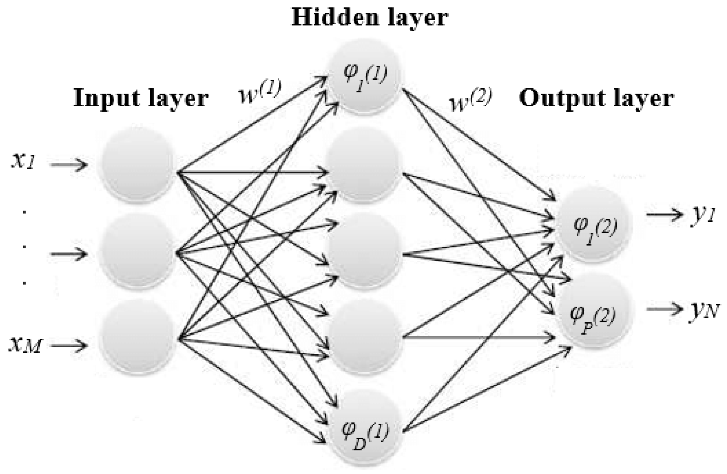
Research into the neural networks (NNs) is quite broad and several research issues and challenges exist. Nevertheless, multilayer perceptrons (MLP) is the predominant version of neural networks often in practical deployment. Figure 4 provides a visual of the MLP archetype with a simple two-layer system. The variables of the input vector x are units (neurons) in the input layer, i(1) are the hidden layer units, and i(2) are the output layer units, that outputs y. The functionality of the units in each layer are modified the nonlinear function of the actions executed in the previous layer. In ML, (.) is termed as an activation function. In NNs, the activation function receives the linear input data and converts them to non-linear data. For estimation assignment, a linear activation function is used, and for multiclass classification, a softmax activation function is used [55,57]. Equation (12) denotes the form of classification or regression task:
f(x, w(1), w(2)) = (2)((1)(xT w(1))T w(2))
where w(1) = (w1(1), …, wM(1))T, (1) = (1(1), …,D(1))T, w(2) = (w1(2), …, wD(2))T, and (2) = (1(2), …,P(2))T.
When presented with an adequate hidden unit, an MLP having a minimum of two layers can equate a random mapping originating from a finite input domain to a finite output domain [21,22,23]. Nevertheless, discovering the ideal set of weights w for an MLP can be modelled as NP-complete optimization problem [24]. Several algorithms are used to training neural network models such as stochastic gradient descent, adaptive delta, adaptive gradient, adaptive moment estimation, Nesterov’s accelerated gradient, and RMSprob. The issues of generalization and overfitting reduction can be addressed via weight decay, weight-sharing, early stopping, Bayesian fitting of neural nets, dropout, and generative pre-training [22,29]. A two-layer MLP are equipped with controlled representation and generalization. Hence, densely denoted functions with l layers admits an exponential size with l-1 layers. Consequently, a different scheme might be considering an MLP having more a single hidden layer, i.e., a deep NN (DNN), the various high-level functionality is accessed by the low-level features [10,53]. NNs algorithms have assumed the de-facto model in ML models which has been buoyed by the overwhelming outcomes [57]. Ma et al. [26] suggested a strategy of estimating the states of IoT components using on an artificial NN. The analyzed architecture of the NN is a fusion of MLP and a probabilistic NN. Ghaderi et al. [21] deployed an MLP for processing health data. Additionally, MLP has been deployed for future energy consumption via predicting future energy data energy data generation and how the redundancy of this data will be removed [21,26,48].
Syafrudin et. al. [64] developed a real-time monitoring system that utilizes IoT-based sensors to collects temperature, humidity, accelerometer, and gyroscope data, and big data processing; where a hybrid prediction model that consists of DBSCAN-based outlier detection is used and Random Forest classification. DBSCAN was used to separate outliers from normal sensor data, while Random Forest was utilized to predict faults—given the sensor data as input. The proposed model was evaluated and tested at an automotive manufacturing assembly line in Korea. The results showed that IoT-based sensors and the proposed big data processing system are sufficient to monitor the manufacturing process. Furthermore, the proposed hybrid prediction model has better fault prediction accuracy than other models given the sensor data as input. The proposed system is expected to support management by improving decision-making and will help prevent unexpected losses caused by faults during the manufacturing process.
Satija et. al. [65] design and development of a light-weight ECG SQA method for automatically classifying the acquired ECG signal into acceptable or unacceptable class and real-time implementation of proposed IoT-enabled ECG monitoring framework using ECG sensors, Arduino, Android phone, Bluetooth, and cloud server. The proposed quality-aware ECG monitoring system consists of three modules: (1) ECG signal sensing module, (2) automated signal quality assessment (SQA) module, and (3) signal-quality aware (SQAw) ECG analysis and transmission module. The proposed framework is tested and validated using the ECG signals taken from the MIT-BIH arrhythmia and Physionet challenge databases and the real-time recorded ECG signals under different physical activities. Experimental results show that the proposed SQA method achieves promising results in identifying the unacceptable quality of ECG signals and outperforms existing methods based on the morphological and RR interval features and machine learning approaches. This paper further shows that the transmission of acceptable quality of ECG signals can significantly improve the battery lifetime of IoT-enabled devices. The proposed quality aware IoT paradigm has great potential for assessing the clinical acceptability of ECG signals for the improvement of accuracy and reliability of unsupervised diagnosis system.

3. Research Trends and Open Issues

3.1. Privacy and Security

The IoT consists of plethora of divergent network nodes interconnected to one another and transmitting vast volumes of data. IoT use cases can be categorized into various cases based on specific characters and attributes. For IoT use-cases to be implemented correctly for data analysis, certain issues must be addressed. Firstly, the privacy of the collected data must be guided jealously as the data may include highly sensitive data such as personal, health and business-related data. Hence, this privacy issue must be addressed. Secondly, as the number of data source increases alongside the simplicity of IoT hardware, it has become imperative to study security constraints, such as network security and data encryption. It is plausible that if adequate measures are not incorporated into the strategy and execution of IoT devices, it may result in an unsecured network.

3.2. Real-Time Data Analytics

Based on the unique attributes of smart data, analytic algorithms are equipped to deal with big data. Concisely, the IoT needs models that can study data emanating from various sources in real-time. Many researchers have attempted to tackle this issue. In the presence of a large dataset, deep learning algorithms can attain a high degree of accuracy if given enough training time. Unfortunately, deep learning algorithms are easily corrupted by noisy smart data. Similarly, NN-based algorithms are subject to inaccurate analysis. Equivalently, semi-supervised algorithms, which model a small amount of identified data with a huge amount of unidentified data, can be helpful in IoT data analysis.

4. Conclusions and Recommendations

This study addresses the supervised and unsupervised machine learning techniques that are considered the main pillars of the IoT smart data analysis. Obtaining optimal results in smart data analysis requires an in-depth understanding of data structure, discovering abnormal data points, estimating parameters, estimating categories and extracting salient data features. For sequenced data prediction and classification, the linear regression and SVM methods are the two most frequently applied algorithms. The goals of the deployed models lie in processing and training high velocity data. Another fast training algorithm is the classification and regression tree. Discovering abnormal data points and irregularities in smart data, these notable algorithms can be executed. Namely, the one-class SVM or PCA-based anomaly detection method. Both can train anomalies and noisy data with a high degree of accuracy. The SVM is one of the commonly used classification algorithms. The algorithm has the capacity to handle huge dataset classifying them into various categories. Based on this unique attribute of SVM, it is widely deployed in areas where the data has huge volume, data sources coming from various sources, and where smart data processing algorithms are needed. To discover the structure of unlabeled data, clustering algorithms can provide the most appropriate tools. K-means is the most widely used clustering algorithm and it is equipped to work with huge data volume cutting across a broad spectrum of data source. PCA and CCA are the two most prominent algorithms features extraction. Furthermore, CCA has the capacity to depict a correlation between two groups of data. A type of PCA or CCA is ideal to locate data anomalies. To predict the categories of data, neural networks are suitable learning models for function approximation problems. Moreover, because smart data should be accurate and require a long training time, a multi-class neural network could provide an appropriate solution. Research on the ML indicate that several challenges remain. This article has highlighted some shortcomings and challenges that exist with respect to some aspects of supervised and unsupervised machine learning techniques, as well as future research that may prove beneficial in pursuing this vision as a useful technology.

Author Contributions

As the first author, M.H.A. wrote the main parts and conceptualization the first draft of this paper; methodology, M.H.A. and A.H.K.; project administration K.Y.; S.A.C. revised the final version of paper. All authors have read and agreed to the published version of the manuscript.

Funding

This research received no external funding.

Conflicts of Interest

The authors declare no conflict of interest.

References

  1. Sharakhina, L.V.; Skvortsova, V. Big Data, Smart Data in Effective Communication Strategies Development. In Proceedings of the 2019 Communication Strategies in Digital Society Workshop (ComSDS), Saint Petersburg, Russia, 10 April 2019; pp. 7–10. [Google Scholar]
  2. Al-Fuqaha, A.; Guizani, M.; Mohammadi, M.; Aledhari, M.; Ayyash, M. Internet of things: A survey on enabling technologies, protocols, and applications. IEEE Commun. Surv. Tutor. 2015, 17, 2347–2376. [Google Scholar] [CrossRef]
  3. Alzubi, J.; Nayyar, A.; Kumar, A. Machine Learning from Theory to Algorithms: An Overview; Journal of Physics: Conference Series; IOP Publishing: London, UK, 2018; p. 012012. [Google Scholar]
  4. Jagannath, J.; Polosky, N.; Jagannath, A.; Restuccia, F.; Melodia, T. Machine learning for wireless communications in the Internet of things: A comprehensive survey. Ad Hoc Netw. 2019, 101913. [Google Scholar] [CrossRef] [Green Version]
  5. Kashyap, R. Machine Learning for Internet of Things. In Next-Generation Wireless Networks Meet Advanced Machine Learning Applications; IGI Global: Hershey, PA, USA, 2019; pp. 57–83. [Google Scholar]
  6. Masegosa, A.R.; Martínez, A.M.; Ramos-López, D.; Cabañas, R.; Salmerón, A.; Langseth, H.; Nielsen, T.D.; Madsen, A.L. AMIDST: A Java toolbox for scalable probabilistic machine learning. Knowl.-Based Syst. 2019, 163, 595–597. [Google Scholar] [CrossRef] [Green Version]
  7. Buskirk, T.D.; Kirchner, A.; Eck, A.; Signorino, C.S. An introduction to machine learning methods for survey researchers. Surv. Pract. 2018, 11, 2718. [Google Scholar] [CrossRef] [Green Version]
  8. Luong, N.C.; Hoang, D.T.; Gong, S.; Niyato, D.; Wang, P.; Liang, Y.-C.; Kim, D.I. Applications of deep reinforcement learning in communications and networking: A survey. IEEE Commun. Surv. Tutor. 2019, 21, 3133–3174. [Google Scholar] [CrossRef] [Green Version]
  9. Schrider, D.R.; Kern, A.D. Supervised machine learning for population genetics: A new paradigm. Trends Genet. 2018, 34, 301–312. [Google Scholar] [CrossRef] [Green Version]
  10. Lee, J.H.; Shin, J.; Realff, M.J. Machine learning: Overview of the recent progresses and implications for the process systems engineering field. Comput. Chem. Eng. 2018, 114, 111–121. [Google Scholar] [CrossRef]
  11. Singh, A.; Thakur, N.; Sharma, A. A review of supervised machine learning algorithms. In Proceedings of the 2016 3rd International Conference on Computing for Sustainable Global Development (INDIACom), New Delhi, India, 16–18 March 2016; pp. 1310–1315. [Google Scholar]
  12. Osisanwo, F.; Akinsola, J.; Awodele, O.; Hinmikaiye, J.; Olakanmi, O.; Akinjobi, J. Supervised machine learning algorithms: Classification and comparison. Int. J. Comput. Trends. Technol. 2017, 48, 128–138. [Google Scholar]
  13. Qu, G.; Li, N. Accelerated distributed nesterov gradient descent for smooth and strongly convex functions. In Proceedings of the 2016 54th Annual Allerton Conference on Communication, Control, and Computing (Allerton), Monticello, IL, USA, 27–30 September 2016; pp. 209–216. [Google Scholar]
  14. Lee, J.; Stanley, M.; Spanias, A.; Tepedelenlioglu, C. Integrating machine learning in embedded sensor systems for Internet-of-Things applications. In Proceedings of the 2016 IEEE International Symposium on Signal Processing and Information Technology (ISSPIT), Limassol, Cyprus, 12–14 December 2016; pp. 290–294. [Google Scholar]
  15. Kanj, S.; Abdallah, F.; Denoeux, T.; Tout, K. Editing training data for multi-label classification with the k-nearest neighbor rule. Pattern Anal. Appl. 2016, 19, 145–161. [Google Scholar] [CrossRef] [Green Version]
  16. Maillo, J.; Ramírez, S.; Triguero, I.; Herrera, F. kNN-IS: An Iterative Spark-based design of the k-Nearest Neighbors classifier for big data. Knowl.-Based Syst. 2017, 117, 3–15. [Google Scholar] [CrossRef] [Green Version]
  17. Chomboon, K.; Chujai, P.; Teerarassamee, P.; Kerdprasop, K.; Kerdprasop, N. An empirical study of distance metrics for k-nearest neighbor algorithm. In Proceedings of the 3rd International Conference on Industrial Application Engineering, Kitakyushu, Japan, 28–31 March 2015; pp. 1–6. [Google Scholar]
  18. Prasath, V.; Alfeilat, H.A.A.; Lasassmeh, O.; Hassanat, A.; Tarawneh, A.S. Distance and Similarity Measures Effect on the Performance of K-Nearest Neighbor Classifier—A Review. arXiv 2017, arXiv:1708.04321. [Google Scholar]
  19. Berisha, V.; Wisler, A.; Hero, A.O.; Spanias, A. Empirically estimable classification bounds based on a nonparametric divergence measure. IEEE Trans. Signal Process. 2015, 64, 580–591. [Google Scholar] [CrossRef] [PubMed] [Green Version]
  20. Azar, A.T.; Hassanien, A.E. Dimensionality reduction of medical big data using neural-fuzzy classifier. Soft Comput. 2015, 19, 1115–1127. [Google Scholar] [CrossRef]
  21. Ghaderi, A.; Frounchi, J.; Farnam, A. Machine learning-based signal processing using physiological signals for stress detection. In Proceedings of the 2015 22nd Iranian Conference on Biomedical Engineering (ICBME), Tehran, Iran, 25–27 November 2015; pp. 93–98. [Google Scholar]
  22. Sharmila, A.; Geethanjali, P. DWT based detection of epileptic seizure from EEG signals using naive Bayes and k-NN classifiers. IEEE Access 2016, 4, 7716–7727. [Google Scholar] [CrossRef]
  23. Garcia, L.P.; de Carvalho, A.C.; Lorena, A.C. Effect of label noise in the complexity of classification problems. Neurocomputing 2015, 160, 108–119. [Google Scholar] [CrossRef]
  24. Lu, W.; Du, X.; Hadjieleftheriou, M.; Ooi, B.C. Efficiently Supporting Edit Distance Based String Similarity Search Using B+ -Trees. IEEE Trans. Knowl. Data Eng. 2014, 26, 2983–2996. [Google Scholar] [CrossRef]
  25. Do, C.-T.; Douzal-Chouakria, A.; Marié, S.; Rombaut, M. Multiple Metric Learning for large margin kNN Classification of time series. In Proceedings of the 2015 23rd European Signal Processing Conference (EUSIPCO), Nice, France, 31 August–4 September 2015; pp. 2346–2350. [Google Scholar]
  26. Ma, X.; Wu, Y.-J.; Wang, Y.; Chen, F.; Liu, J. Mining smart card data for transit riders’ travel patterns. Transp. Res. Part C Emerg. Technol. 2013, 36, 1–12. [Google Scholar] [CrossRef]
  27. Wang, H.; Zhang, Y.; Waytowich, N.R.; Krusienski, D.J.; Zhou, G.; Jin, J.; Wang, X.; Cichocki, A. Discriminative feature extraction via multivariate linear regression for SSVEP-based BCI. IEEE Trans. Neural Syst. Rehabil. Eng. 2016, 24, 532–541. [Google Scholar] [CrossRef]
  28. Hilbe, J.M. Practical Guide to Logistic Regression; Chapman and Hall/CRC: Boca Raton, FL, USA, 2016. [Google Scholar]
  29. Mahdavinejad, M.S.; Rezvan, M.; Barekatain, M.; Adibi, P.; Barnaghi, P.; Sheth, A.P. Machine learning for Internet of Things data analysis: A survey. Digit. Commun. Netw. 2018, 4, 161–175. [Google Scholar] [CrossRef]
  30. Jadhav, S.D.; Channe, H. Comparative study of K-NN, naive Bayes and decision tree classification techniques. Int. J. Sci. Res. 2016, 5, 1842–1845. [Google Scholar]
  31. Xu, S. Bayesian Naïve Bayes classifiers to text classification. J. Inf. Sci. 2018, 44, 48–59. [Google Scholar] [CrossRef]
  32. Singh, G.; Kumar, B.; Gaur, L.; Tyagi, A. Comparison between Multinomial and Bernoulli Naïve Bayes for Text Classification. In Proceedings of the 2019 International Conference on Automation, Computational and Technology Management (ICACTM), London, UK, 24–26 April 2019; pp. 593–596. [Google Scholar]
  33. Pham, B.T.; Prakash, I.; Jaafari, A.; Bui, D.T. Spatial prediction of rainfall-induced landslides using aggregating one-dependence estimators classifier. J. Indian Soc. Remote Sens. 2018, 46, 1457–1470. [Google Scholar] [CrossRef]
  34. Han, W.; Gu, Y.; Zhang, Y.; Zheng, L. Data driven quantitative trust model for the internet of agricultural things. In Proceedings of the 2014 International Conference on the Internet of Things (IOT), Cambridge, MA, USA, 6–8 October 2014; pp. 31–36. [Google Scholar]
  35. Cherian, V.; Bindu, M. Heart disease prediction using Naive Bayes algorithm and Laplace Smoothing technique. Int. J. Comput. Sci. Trends Technol. 2017, 5. [Google Scholar]
  36. Weichenthal, S.; Van Ryswyk, K.; Goldstein, A.; Bagg, S.; Shekkarizfard, M.; Hatzopoulou, M. A land use regression model for ambient ultrafine particles in Montreal, Canada: A comparison of linear regression and a machine learning approach. Environ. Res. 2016, 146, 65–72. [Google Scholar] [CrossRef] [Green Version]
  37. Hoffmann, J.P.; Shafer, K. Linear Regression Analysis; NASW Press: Washington, DC, USA, 2015. [Google Scholar]
  38. Montgomery, D.C.; Peck, E.A.; Vining, G.G. Introduction to Linear Regression Analysis; John Wiley & Sons: Hoboken, NJ, USA, 2012; Volume 821. [Google Scholar]
  39. Robert, C. Machine Learning, a Probabilistic Perspective; Taylor & Francis: Abingdon, UK, 2014. [Google Scholar]
  40. Derguech, W.; Bruke, E.; Curry, E. An autonomic approach to real-time predictive analytics using open data and internet of things. In Proceedings of the 2014 IEEE 11th Intl Conf on Ubiquitous Intelligence and Computing and 2014 IEEE 11th Intl Conf on Autonomic and Trusted Computing and 2014 IEEE 14th International Conference on Scalable Computing and Communications and Its Associated Workshops, Bali, Indonesia, 9–12 December 2014; pp. 204–211. [Google Scholar]
  41. Glorot, X.; Bengio, Y. Understanding the difficulty of training deep feedforward neural networks. In Proceedings of the Thirteenth International Conference on Artificial Intelligence and Statistics, Sardinia, Italy, 13–15 May 2010; pp. 249–256. [Google Scholar]
  42. Ding, S.; Qi, B.; Tan, H. An overview on theory and algorithm of support vector machines. J. Univ. Electron. Sci. Technol. China 2011, 40, 2–10. [Google Scholar]
  43. Nikam, S.S. A comparative study of classification techniques in data mining algorithms. Orient. J. Comput. Sci. Technol. 2015, 8, 13–19. [Google Scholar]
  44. Alber, M.; Zimmert, J.; Dogan, U.; Kloft, M. Distributed optimization of multi-class SVMs. PLoS ONE 2017, 12, e0178161. [Google Scholar] [CrossRef] [Green Version]
  45. Ponte, P.; Melko, R.G. Kernel methods for interpretable machine learning of order parameters. Phys. Rev. B 2017, 96, 205146. [Google Scholar] [CrossRef] [Green Version]
  46. Utkin, L.V.; Chekh, A.I.; Zhuk, Y.A. Binary classification SVM-based algorithms with interval-valued training data using triangular and Epanechnikov kernels. Neural Netw. 2016, 80, 53–66. [Google Scholar] [CrossRef]
  47. Díaz-Morales, R.; Navia-Vázquez, Á. Distributed Nonlinear Semiparametric Support Vector Machine for Big Data Applications on Spark Frameworks. IEEE Trans. Syst. Man Cybern. Syst. 2018, 1–12. [Google Scholar] [CrossRef]
  48. Lee, C.-P.; Roth, D. Distributed box-constrained quadratic optimization for dual linear SVM. In Proceedings of the International Conference on Machine Learning, Lille, France, 6–11 July 2015; pp. 987–996. [Google Scholar]
  49. Huang, X.; Shi, L.; Suykens, J.A. Sequential minimal optimization for SVM with pinball loss. Neurocomputing 2015, 149, 1596–1603. [Google Scholar] [CrossRef]
  50. Azim, R.; Rahman, W.; Karim, M.F. Bangla Hand-Written Character Recognition Using Support Vector Machine. Int. J. Eng. Works 2016, 3, 36–46. [Google Scholar]
  51. Liu, P.; Choo, K.-K.R.; Wang, L.; Huang, F. SVM or deep learning? A comparative study on remote sensing image classification. Soft Comput. 2017, 21, 7053–7065. [Google Scholar] [CrossRef]
  52. Cang, Z.; Mu, L.; Wu, K.; Opron, K.; Xia, K.; Wei, G.-W. A topological approach for protein classification. Comput. Math. Biophys. 2015, 3. [Google Scholar] [CrossRef]
  53. Wahab, O.A.; Mourad, A.; Otrok, H.; Bentahar, J. CEAP: SVM-based intelligent detection model for clustered vehicular ad hoc networks. Expert Syst. Appl. 2016, 50, 40–54. [Google Scholar] [CrossRef]
  54. Khan, M.A.; Khan, A.; Khan, M.N.; Anwar, S. A novel learning method to classify data streams in the internet of things. In Proceedings of the 2014 National Software Engineering Conference, Rawalpindi, Pakistan, 11–12 November 2014; pp. 61–66. [Google Scholar]
  55. Nikravesh, A.Y.; Ajila, S.A.; Lung, C.-H.; Ding, W. Mobile network traffic prediction using MLP, MLPWD, and SVM. In Proceedings of the 2016 IEEE International Congress on Big Data (BigData Congress), San Francisco, CA, USA, 27 June–2 July 2016; pp. 402–409. [Google Scholar]
  56. Breiman, L. Classification and Regression Trees; Routledge: Abingdon, UK, 2017. [Google Scholar]
  57. Krzywinski, M.; Altman, N. Points of Significance: Classification and Regression Trees; Nature Publishing Group: Berlin, Germany, 2017. [Google Scholar]
  58. Wuest, T.; Weimer, D.; Irgens, C.; Thoben, K.-D. Machine learning in manufacturing: Advantages, challenges, and applications. Prod. Manuf. Res. 2016, 4, 23–45. [Google Scholar] [CrossRef] [Green Version]
  59. Hagenauer, J.; Helbich, M. A comparative study of machine learning classifiers for modeling travel mode choice. Expert Syst. Appl. 2017, 78, 273–282. [Google Scholar] [CrossRef]
  60. Belgiu, M.; Drăguţ, L. Random forest in remote sensing: A review of applications and future directions. ISPRS J. Photogramm. Remote Sens. 2016, 114, 24–31. [Google Scholar] [CrossRef]
  61. Biau, G.; Scornet, E. A random forest guided tour. Test 2016, 25, 197–227. [Google Scholar] [CrossRef] [Green Version]
  62. Selvi, S.T.; Karthikeyan, P.; Vincent, A.; Abinaya, V.; Neeraja, G.; Deepika, R. Text categorization using Rocchio algorithm and random forest algorithm. In Proceedings of the 2016 Eighth International Conference on Advanced Computing (ICoAC), Chennai, India, 19–21 January 2017; pp. 7–12. [Google Scholar]
  63. Hassan, A.R.; Bhuiyan, M.I.H. Computer-aided sleep staging using complete ensemble empirical mode decomposition with adaptive noise and bootstrap aggregating. Biomed. Signal Process. Control 2016, 24, 1–10. [Google Scholar] [CrossRef]
  64. Syafrudin, M.; Alfian, G.; Fitriyani, N.; Rhee, J. Performance Analysis of IoT-Based Sensor, Big Data Processing, and Machine Learning Model for Real-Time Monitoring System in Automotive Manufacturing. Sensors 2018, 18, 2946. [Google Scholar] [CrossRef] [PubMed] [Green Version]
  65. Satija, U.; Ramkumar, B.; Manikandan, M.S. Real-Time Signal Quality-Aware ECG Telemetry System for IoT-Based Health Care Monitoring. IEEE Internet Things J. 2017, 4, 815–823. [Google Scholar] [CrossRef]
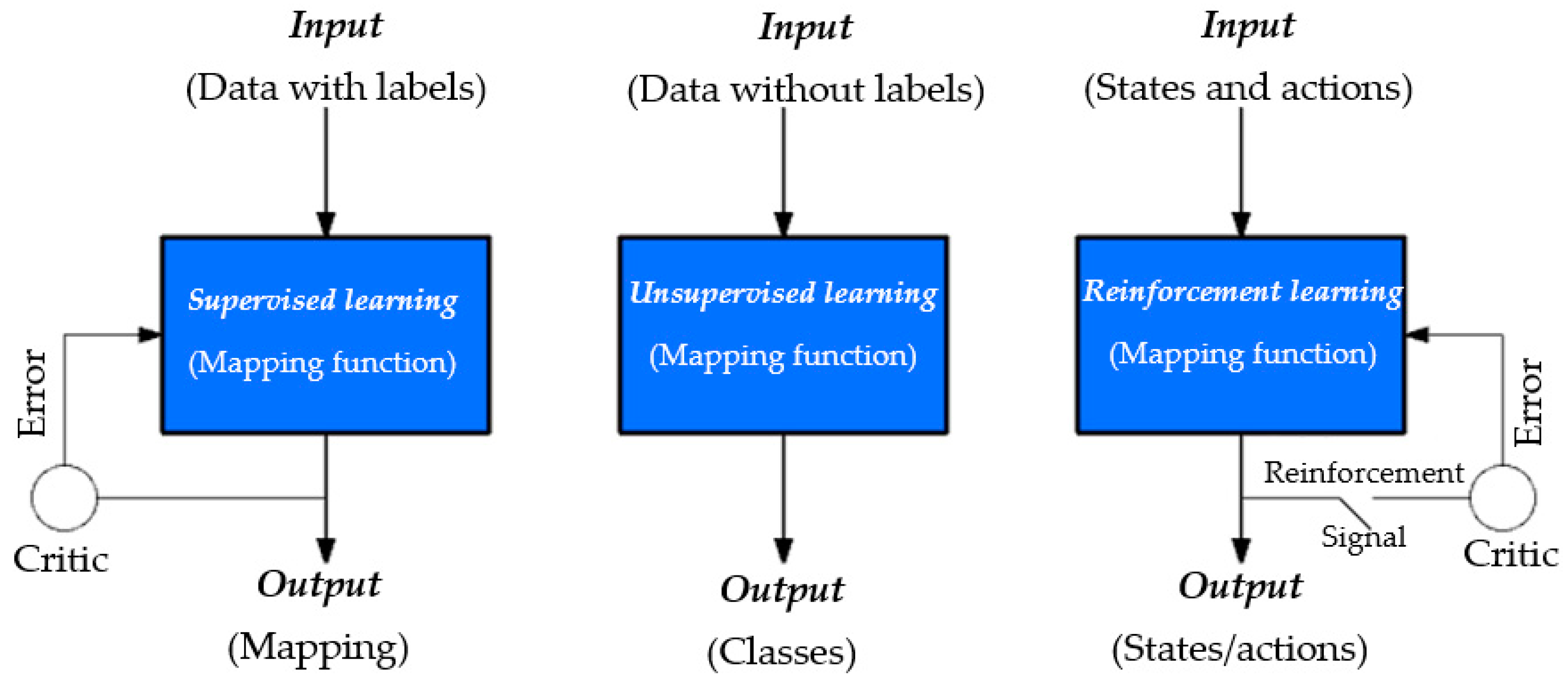
Figure 1. Classification of learning models.
Symmetry 12 00088 g001
Figure 2. Summarized taxonomy of supervised and unsupervised ML algorithms.
Symmetry 12 00088 g002
Figure 3. A simple KNN model for different values of k.
Symmetry 12 00088 g003
Figure 4. A visual of the MLP archetype with a simple two-layer model.
Symmetry 12 00088 g004
Table 1. Summarized comparison of the basis and notable attributes, as well as advantages and limitations.
Data Analysis TasksML AlgorithmAdvantagesDisadvantages
ClassificationKNN
  • Very simple implementation.
  • New data can be added seamlessly.
  • Robust against noisy training data.
  • It has the capability to modeling complex classification problem by a collection of less complex local approximation.
  • Maintain the information that presents in the training data.
  • Does not work well with large dataset.
  • Sensitive to unbalanced training data.
  • It is supervised lazy learner.
  • Memory usage cost.
Naive Bayes
  • Resulting interpretable model.
  • Computational efficiency and highly scalable.
  • Good classification performance.
  • Require a small number of data points to be trained.
  • It can deal with high-dimensional data points.
  • It assumes that all the features are mutually independent. However, in real life, it is rarely that there is no correlation between features in raw data, which in turn leads to negatively on the classification accuracy.
RegressionLinear Regression
  • Model development is rapid and straightforward.
  • Useful when the relationship to be modeled is not extremely complex and if don’t have a lot of data.
  • Applicable only if the solution is linear. In many real-life scenarios, it may not be the case.
  • Algorithm assumes the input residuals (error) to be normally distributed but may not be satisfied always.
Combining Classification and RegressionSVM
  • Regularization capabilities.
  • Handles non-linear data efficiently.
  • Solves both Classification and Regression problems.
  • Stability.
  • Provide better generalization capabilities.
  • Choosing an appropriate Kernel function is difficult.
  • Extensive memory requirement.
  • Requires Feature Scaling.
  • Time-consuming training.
  • Difficult to interpret.
Random Forest
  • It is considered one of the most robustness and accurate computational learning algorithms
  • Good performance on many problem instances including non-linear.
  • It has the capability of detect outliers and anomalies in knowledgeable data.
  • Overfitting can easily occur.
  • Need to determine the number of trees.
  • Small perturbation in data can significantly modify the tree’s structure, which in turn leads to produce inaccurate interpretations.
Bootstrap Aggregating
  • They often provide better calcification accuracy results than those obtained by individual machine learning.
  • Increasing of computational complexity.
  • loss of interaction among the individual networks during learning.