Computer-Aided Laser-Fiber Output Beam 3D Spatial and Angular Design

Abstract

Multiple laser beams and single-mode optical fibers output can be approximated by assuming that the emitted light has a symmetrical Gaussian intensity profile, which corresponds to the transverse electromagnetic mode (TEM₀₀), which is designated as a Gaussian beam. Current free-accessible design tools are limited to the spatial analysis of the beams, in general, and to the intensity, in particular, and to the graphical visualization in 2D with very limited options. In this work, a novel a computer-aided laser-fiber output beam TEM₀₀ designer, CATEM00, is presented based on the 3D representations typically provided by camera beam profilers, and on the fundamentals of the wave theory of light, including diverse flexibility capabilities for graphical manipulation and parameter comprehension both in terms of spatial behavior and in angular confinement. It must be highlighted that not only is the spatial limitation design of light impact relevant in TEM₀₀ applications but, also, the angle with which the light reaches the target. Hence, the availability of capabilities of phase design in TEM₀₀ following the paraxial limitations is highly convenient. Results and discussion in terms of intensity, power, divergence and wave fronts are presented considering a set of study cases, showing its coherence with Gaussian beam theory.

1. Introduction

Most laser applications consist of the impact of light on objects or materials on a given limited surface with a striking angle and spatial distribution of power strictly bounded. The objects to impact can be both light detection equipment for information systems, such as cameras, or industrial or biological materials to be drilled, melted, or heated [1]. The quality of the performance of the light impact highly depends on the features of the beam of the light source and the way these features change across the beam and along the optical axis as it propagates in free space. Particularly, the transverse electromagnetic mode (TEM₀₀) describes the observed output of many lasers, which are designed and tuned to emit this mode, and it also approximates the light of the output of a single-mode optical fiber [2]. The ideal TEM₀₀ beam presents an intensity profile that corresponds to a Gaussian expression and, thus, it is also known as a Gaussian beam [3]. In TEM₀₀ mode, the light beam presents an intensity transverse section that is maximum in the center and that it characterized by its revolution symmetry around the optical axis. Analogously, the angular deviation of the beam reaches its lowest value in the optical axis and it is increased in its surroundings, ruled by the paraxial approximation, also presenting symmetry with respect to this axis. Hence, both the space and angular parameters of the light beam, i.e., intensity, the power distribution and divergence, and wave fronts, respectively, of the TEM₀₀ profile are featured by its symmetry around the optical axis, which is convenient and demanded in most related applications.

TEM₀₀ mode with Gaussian beam applications are included within those of paraxial waves. Paraxial waves are of relevance in applications where it is necessary to achieve the propagation of light in free space not only with a spatial confinement, but also with an angular confinement. Spatial confinement refers to the characteristic of the wave of being limited to a specific region of space while the angular confinement corresponds to the condition of the normal directions to the wave fronts that imposes small angles with the optical axis or axial axis z. In this way, the beam power is concentrated in a small cone around the optical axis. There are different parameters describing the light beam both in terms of spatial and angular behavior, joined to different concepts of intensity, power, divergence and wave fronts. In diverse application areas ranging from medicine, e.g., ophthalmic laser surgery [4], to industry, e.g., fusion and material drilling [5], and military applications, e.g., weapons and signals detectors, the correct understanding of the beam parameters is critical for its design and use. Furthermore, the precise understanding of the light source parameters associated to the performance of the laser source is relevant to detect the need for tuning and profiling of the beam equipment, which is typically related to the measurement of symmetry and smoothness [1].

There are diverse computer-aided tools for TEM₀₀ beam features that have empowered researchers and engineers to design lasers to the highest quality. Particularly, in regard to TEM₀₀ beam computer-aided open-source designers, there exist many beam software packages offering analytical and visual results of diverse beams featuring parameters such as spot size, beam waist, and divergence on the basis of main characteristics of the light source performance, such as frequency and Rayleigh distance. This is the case of [6,7,8], which are the major open-accessible software in the field to the best of the authors’ knowledge. Nevertheless, these tools present different deficiencies that reduce the manageability, intuition, and versatility. Mainly, these deficiencies arise from the limitation to spatial analysis of the beam, typically to intensity features, and to the static visualization of its profile, including non- or very reduced flexibility for graphical design in 3D and 2D. In this sense, [6] just offers the possibility to visualize in 2D the Gaussian beam waist in different positions of the optical axis. Additionally, in this regard, [7] allows the visualization of the Gaussian beam only in the spatial dimension, and not in the angular one. Moreover, the majority of available tools simply consist of analytical calculators for power and intensity study and no graphical user interfaces for both visual and quantitative analyses are found. In this sense, for example, [8] only offers the analytical end value of the power of the Gaussian beam as a function of position and distance.

In this work, a computer-aided laser-fiber output beam for 3D spatial and angular design tool, CATEM00, is developed in MATLAB [9], integrated in a simplified graphical user interface (GUI), following recent published applications in optics and electronics [10,11]. Additionally, CATEM00 is made accessible to the scientific community in [12] as well as in the Supplementary Files attached to this paper. The contribution of this work is highlighted as follows:

• Spatial and angular beam TEM₀₀ design. The previous works that can be currently found in the same area mainly focus on the analysis of the intensity of the Gaussian beam. The proposal in this work offers the possibility to consider a design based on spatial characteristics, such as intensity, power, divergence, as well as on angular characteristics. In particular, the beam can be configured based on wave fronts, and, therefore, it performs not only considering the intensity or power that has to impact on a target zone, but also with the angle with which it will impact on said target zone. The relevance of simultaneous design in both spatial and angular features allows a complete characterization of the beam, which is necessary in high-precision applications.
• Intuitive and flexible GUI. CATEM00 allows the design of TEM₀₀ beams based on the complex wave theory intuitively, both in the comprehension and introduction of the parameters that govern said theory, and in the visualization and interpretation of the results. Thus, the tool allows a direct and simplified design based on the key parameters in both the spatial and angular dimensions, such as the Rayleigh distance and the separation to the optical axis. In addition, the graphical user interface offers the necessary flexibility in determining the area around the optical axis where the paraxial wave approximation is considered. Only through this option an adapted beam design can be made for each application in terms of angular characteristics.
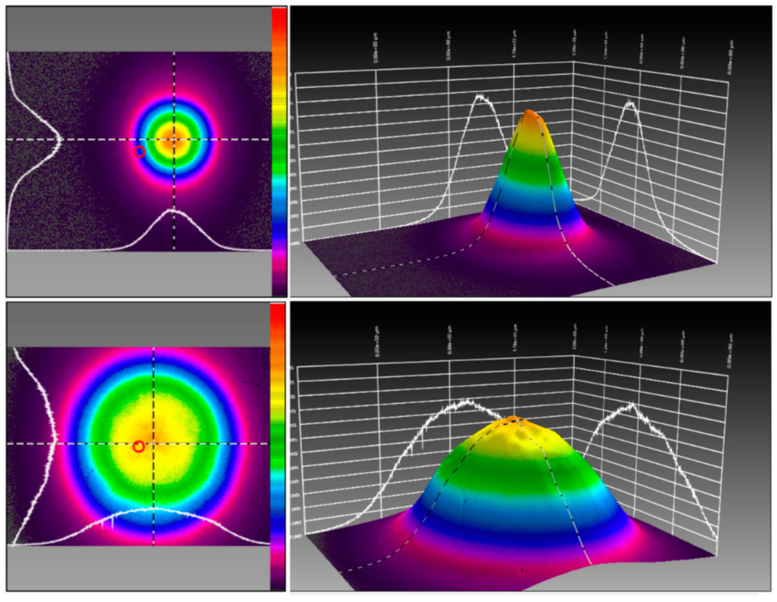
• Visual 2D and 3D design: Unlike other Gaussian beam design tools, the proposal of this work allows simultaneous design in both 3D and 2D following scaled intensity contour schemes for the measured parameters of intensity, power and divergence. In this way, the design result is visually assimilated with the outputs of beam profiling tools for light sources tuning in the operational phase, as obtained, for example, in the case of intensity, with cameras of beam profiling like Spiron SP907 and BeamMic software from Ophir, as shown in Figure 1 [13]. In addition, on existing tuning tools, the visualizations can be rotated at the discretion of the designer and be arranged with the choice of azimuth, elevation, and convenient distance in each application.
• Quantitative results extracted from visual representations of the beam and supporting analysis. The quantitative value at each point of representation of each parameter in design can be extracted directly by clicking on it. In addition, based on the chosen parameters, for the design of the beam in intensity, its characterization in far and near-field is provided, and also for power design, the analysis of power concentrated in a fixed section in the space is displayed. These diagrams are intended to facilitate the choice of input data based on their variation in ranges.
• Freely-available tool. As pointed out above, the proposal is accessible in [12] as well as in the Supplementary Files attached to this paper, with the purpose of facilitating engineers and researchers in the area tools to improve and facilitate the design and comprehension of the spatial and angular design of TEM₀₀ mode.

Finally, it must be highlighted here that quality of any laser-fiber output defined by a TEM₀₀ is directly related to the symmetry of its spatial and angular features, whose guarantee and knowledge is the end purpose of this work. This comes from the fact that the expected symmetry to be found in the impact target in commented critical applications such as ophthalmic laser surgery, strictly depends on the symmetry of the light source beam of impact and thus, designing and testing the beam according to symmetry final outcome is extremely relevant. Hence, with this work, authors aim to make a further step in the symmetry research in the optical field.

The rest of the paper is structured as follows: In Section 2, the main principles and definitions related to the TEM₀₀ mode are presented and the description of the fundamentals of both spatial and angular dimension for its design are introduced. Section 3 is devoted to the explanation of the proposal, including both the tool performance essentials and the GUI main characteristics and properties. Next, in Section 4 the results and associated discussion are provided. Specifically, Section 4 differentiates the results and discussion in terms of intensity, power, divergence, and wave fronts, and multiple examples are analyzed to validate the performance of the tool according to the wave theory for paraxial waves, in general, and Gaussian beams, in particular. Finally, in Section 5 the main conclusions of the work are drawn.

2. Materials and Methods

2.1. Transverse Electromagnetic Mode TEM₀₀ Principles and Definitions

The complex amplitude of the Gaussian beam is obtained from the wave theory of light as a particular case of the complex amplitude of paraxial waves [14]:

$$U(\overrightarrow{r})=A(\overrightarrow{r})\exp (-jkz)$$

(1)

where k represents the wave number, z corresponds to the optical axis-z and A(r) satisfies:

$${\nabla }_T^{2}A-j2k\frac{\partial A}{\partial z}=0$$

(2)

with the following particular form:

$$A(\overrightarrow{r})=\frac{A_1}{q(z)}\exp \left[-jk\frac{{\rho }^2}{2q(z)}\right],q{(z)}^{}=z-\xi$$

(3)

with ρ the distance to the optical axis, q(z) the so-called q parameter and A₁ a constant value. This expression can be regarded as a space-shifted version of the complex envelope for parabolic waves. Specifically, the shift corresponds to $\xi =-j{z}_0$, and so the complex envelope of the Gaussian beam can be defined as:

$$A(\overrightarrow{r})=\frac{A_1}{q(z)}\exp \left[-jk\frac{{\rho }^2}{2q(z)}\right],q{(z)}^{}=z+j{z}_0$$

(4)

where z₀ denotes the Rayleigh range. Separating the real and imaginary parts of 1/q(z):

$$\frac{1}{q(z)}=\frac{1}{R(z)}-j\frac{\lambda }{\pi W^2(z)}$$

(5)

the key parameters of the Gaussian beam can be deduced, being λ the wavelength. On the one hand, it can be inferred that the width or radius of the Gaussian beam corresponds to:

$$W(z)=W_0{\left[1+{\left(\frac{z}{z_0}\right)}^2\right]}^{1/2}$$

(6)

where W₀ describes the beam waist or radius of the light source:

$$W_0={\left(\frac{\lambda z_0}{\pi }\right)}^{1/2}$$

(7)

Twice the value of the beam waist is known as the spot size or beam initial diameter, and it represents the diameter of the light source. The width of the Gauss beam determines the intensity spreading or spatial confinement from the optical axis.

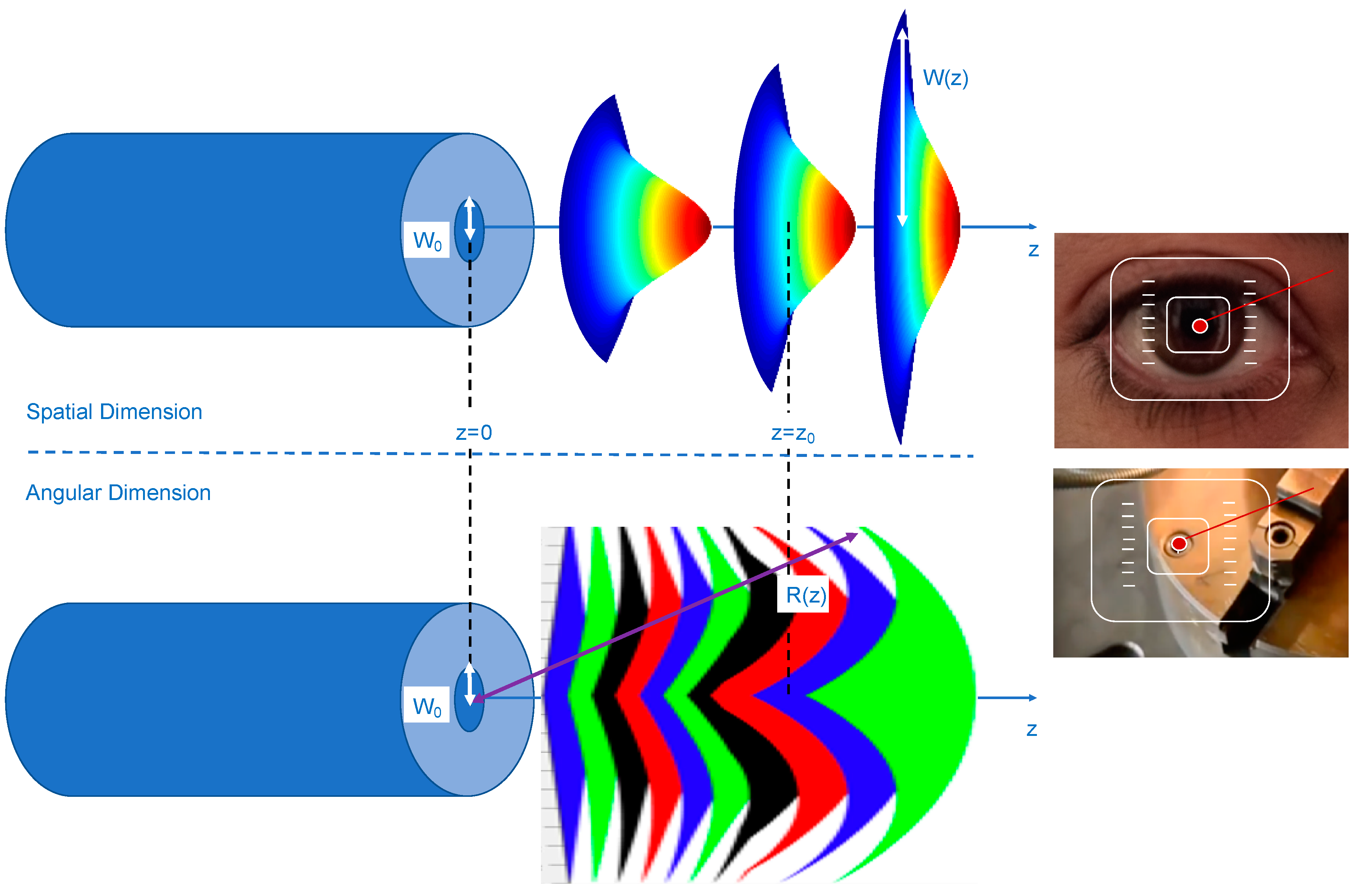
Figure 2 schematically represents the propagation of the TEM₀₀ mode as a function of distance to the light source in the optical axis-z in both spatial and angular dimension. As it can be observed, in the spatial dimension, the form of the intensity corresponds to a Gaussian curve and, thus, the TEM₀₀ laser beams are known as Gaussian beams. Additionally, it can be appreciated that the boundaries of the beam are located around the optical axis, and expands as the beam gets further along in it. The beam waist W₀ and the beam width W(z) are also depicted in Figure 2. As described by Equation (6), the beam diameter of the TEM₀₀ mode is defined as the separation from the center of the beam, where the maximum intensity is always achieved, to the point where the power percentage corresponds to 86.47% approximately. In addition, it can be appreciated in Figure 2 that the beam waist corresponds to the beam width at the light origin.

On the other hand, in regard to the angular definition of the TEM₀₀ beam, the curvature radius of the Gaussian beam it is given by the expression:

$$R(z)=z{\left[1+{\left(\frac{z_0}{z}\right)}^2\right]}^{}$$

(8)

which describes the angular confinement of the beam. In Figure 2, a representation of the wave fronts is presented, as an introduction to their definition, studied in the next section. As shown, the curvature radius R(z) represents the radius of the obtained fronts following the paraxial approximation. Hence, as it can be appreciated, the radio of curvature and, so, the angular confinement of the TEM₀₀ mode, decreases from the light source up to the Rayleigh distance z₀. From the Rayleigh distance, the angular confinement increases. In this way, the wave front evolves from confined plane wave fronts (with infinite value for R(z)) to limited spherical wave fronts (with R(z) = z), that is, confined plane waves in the far-field (with infinite value for R(z)).

In order to easily visualize that the complex amplitude of a Gaussian beam follows a Gauss form it is convenient to substitute q(z) in terms of its module and phase in the amplitude term of Equation (4), and q(z) in terms of W(z) and R(z), i.e., in terms of Equation (5), in the phase term of Equation (4). Hence, the following expression for the complex envelope is obtained:

$$U(\overrightarrow{r})=A_0\frac{W_0}{W(z)}\exp \left(-\frac{{\rho }^2}{W^2(z)}\right)\exp \left(-jkz-jk\frac{{\rho }^2}{2R(z)}+j\zeta \left(z\right)\right)$$

(9)

with A₀ a constant value. From this expression all the properties of the Gaussian beam can be deduced, as it will be summarized as follows.

2.2. Spatial Dimension

First, the beam intensity expression can be obtained from the complex amplitude [14]:

$$I(\overrightarrow{r})={\left|U(\overrightarrow{r})\right|}^2$$

(10)

and substituting Equation (9) in Equation (10):

$$I(\rho ,z)=I_0{\left[\frac{W_0}{W(z)}\right]}^2\exp \left(-\frac{2{\rho }^2}{W^2(z)}\right)$$

(11)

with $I_0={\left|A_0\right|}^2$, where it can be observed that the beam intensity of a Gaussian beam follows a Gaussian expression.

Second, the power is defined as the integral of the optical intensity in a transverse circular plane at a given distance z of infinite radius:

$$P={\displaystyle \underset{0}{\overset{\infty }{\int }}I(\rho ,z)2\pi \rho d\rho }$$

(12)

where substituting Equation (11) gives us the following expression for the power of the Gaussian beam:

$$P=\frac{1}{2}{I}_0\left(\pi W_0^2\right)$$

(13)

Considering this expression, Equation (11) can also be expressed in terms of the power of the Gaussian beam:

$$I(\rho ,z)=\frac{2P}{\pi W^2(z)}\exp \left(-\frac{2{\rho }^2}{W^2(z)}\right)$$

(14)

Also, from the power in a circular cross-section of radius ρ₀, the power fraction on this selected section can be calculated as:

$$\frac{1}{P}{\displaystyle \underset{0}{\overset{{\rho }_0}{\int }}I(\rho ,z)2\pi \rho d\rho }=1-\exp \left(-\frac{2{\rho }^2{}_0}{W^2\left(z\right)}\right)$$

(15)

Third, the divergence or spatial confinement of the beam is given by the beam width described in Equation (6). Specifically, the divergence in far-field corresponds to:

$$W(z)\approx \frac{W_0}{z_0}z=\frac{2}{\pi }\frac{\lambda }{2W_0}={\theta }_{0}z:z>>z_0$$

(16)

where ${\theta }_0$ corresponds to the divergence parameter. Particularly, it is convenient to study the divergence of the beam considering the revolution symmetry of W(z) following Equations (6) and (16) with respect to the optical axis. Moreover, in relation to the divergence of the beam it is relevant to point out the concept of depth of focus, which represents the capacity of the beam to focus light and it corresponds to twice the value of the Rayleigh distance:

$$2z_0=\frac{2\pi W^2{}_0}{\lambda }$$

(17)

2.3. Angular Dimension

From the complex amplitude of the Gaussian beam, Equation (9), the phase of the Gaussian beam can be easily deduced [14]:

$$\phi (\rho ,z)=kz-\zeta \left(z\right)+\frac{k{\rho }^2}{2R(z)}$$

(18)

where it can be inferred that in the optical axis, the phase corresponds to that of plane waves with a slight modification. Wave fronts are the surfaces of constant phase that satisfy:

$$k\left[z+\frac{{\rho }^2}{2R(z)}\right]-\zeta (z)=2\pi q$$

(19)

which, in general for all the points in z, closely describes parabolic surfaces with radius of curvature R(z).

2.4. Incorporating TEM₀₀ Deviations Into the Propagation Model

There exist deviations from theoretical Gaussian beams in the output of real-life lasers and fibers that are also considered in the proposed tool [15,16,17,18]. For example, low-power light beams from helium neon lasers can be a close approximation to TEM₀₀, but it must be noted that as the power of the light source becomes higher, the pumping mechanism becomes more complex and the order of the emitted mode becomes higher and thus, the more the beam deviates from the ideal TEM₀₀. Indeed, although the beam from a well-controlled helium neon laser and other gas lasers is very close to that of a theoretical TEM₀₀ mode, for most lasers, even specifying a TEM₀₀ mode, the output contains some components of higher-order modes that do not propagate according to the theoretical TEM₀₀. Hence, it is necessary to introduce in the proposed tool these deviations from the theoretical Gaussian beam.

Particularly, to accommodate this variance, the M² quality factor (known as the M-squared factor) is generally used in the Gaussian light field to describe the deviation of the laser beam from a theoretical Gaussian beam or theoretical TEM₀₀, and it has also been considered in the presented proposal. This factor can be deduced from the beam parameter product (BPP), which is the result of the TEM₀₀ beam divergence ${\theta }_0$ and waist size W(z). In particular, the M² can be obtained measuring the BPP of a real laser beam (product of the beam’s minimum diameter and far-field divergence) and dividing this value by the BPP of an ideal TEM₀₀ at the same frequency. Hence, the M-squared factor or M² factor is a long-recognized figure of merit used to determine the deviation of the laser beam from a theoretical Gaussian TEM₀₀ that can be defined as:

$$M^2=\frac{W_{0R}{\theta }_{0R}}{W_0{\theta }_0}$$

(20)

where $W_{0R}$ and ${\theta }_{0R}$ are the beam waist and far-field divergence of the real beam, respectively. The M² factor for a theoretical Gaussian beam is equal to the unity, M² = 1 and the beam-waist and beam-divergence product is given by:

$$W_0{\theta }_0=\frac{\lambda }{\pi }$$

(21)

It follows then that for a real laser beam or deviated TEM₀₀:

$$W_{0R}{\theta }_{0R}=\frac{M^2\lambda }{\pi }$$

(22)

All real laser beams have M² values greater than one (M² > 1), although very high-quality beams present values very close to the unity. In all cases, the M² factor affects the characteristics of a laser beam and cannot be neglected in optical designs. Specific values for M² can be found in many common TEM₀₀ light sources. For instance, for helium neon lasers M² is generally lower than 1.1 (M² < 1.1). For ion lasers, the M² typical range goes from 1.1 to 1.3 (1.1 < M² < 1.3). In addition, collimated TEM₀₀ diode laser beams usually have an M² ranging from 1.1 to 1.7 (1.1 < M² < 1.7) and in high-energy multimode lasers, M² can be as high as 25 or 30 (25 < M² < 30).

Once the deviations from the theoretical TEM₀₀ have been analyzed, the propagation model must be redefined accordingly. Specifically, the propagation equations for a real laser beam must now consider the following expressions for the beam radius:

$$W_R(z)=W_{0R}{\left[1+{\left(\frac{z}{z_{0R}}\right)}^2\right]}^{1/2}=W_{0R}{\left[1+{\left(\frac{z\lambda M^2}{\pi W^2{}_{0R}}\right)}^2\right]}^{1/2}$$

(23)

and the radius of curvature:

$$R_R(z)=z{\left[1+{\left(\frac{z_{0R}}{z}\right)}^2\right]}^{1/2}=z{\left[1+{\left(\frac{\pi W^2{}_{0R}}{z\lambda M^2}\right)}^2\right]}^{}$$

(24)

where the Rayleigh distance is transformed to:

$$z_{0R}=\frac{\pi W^2{}_{0R}}{\lambda M^2}$$

(25)

2.5. Laguerre–Gaussian Modes

The TEM₀₀ mode can be regarded as a particular case of Laguerre–Gaussian modes [19]. When a laser light beam has a circularly symmetric profile or its associated cavity is cylindrically symmetric (as in the case of optical fibers too) the propagation model is efficiently described by the Laguerre–Gaussian modal decomposition. The related expressions are expressed in cylindrical coordinates considering generalized Laguerre polynomials. Particularly, each TEM mode is denoted using two integers p (positive or zero) and l, representing the radial index and the azimuthal index, respectively. The general case corresponds to TEM_pl modes and to TEM₀₀ when p and l are zero. The specific form of the complex amplitude for the general case of Laguerre–Gaussian TEM_pl modes corresponds to the following expression:

$$\begin{array}{ll}\hfill U(\overrightarrow{r})& =C^{LG}{}_{lp}\frac{W_0}{W(z)}\exp {\left(-\frac{r\sqrt{2}}{W(z)}\right)}^{{}^{\left|l\right|}}\exp \left(-\frac{r^2}{W^2(z)}\right)L_p^{{}^{\left|l\right|}}\exp \left(-\frac{2r^2}{W^2(z)}\right)\times \\ & \exp \left(-jk\frac{r^2}{2R(z)}\right)\exp \left(-jl\varphi \right)\exp \left(j\psi (z)\right)\end{array}$$

(26)

where $L_p^{{}^{\left|l\right|}}$ indicates the generalized Laguerre polynomials, $C_{lp}^{LG}$ corresponds to a normalization constant, W(z) and R(z) were described in Equations (6) and (8), respectively, for the TEM₀₀, and the Guoy phase along z is:

$$\psi (z)=\left(N+1\right){\tan }^{-1}\left(\frac{z}{z_0}\right)$$

(27)

with N = |l| + 2p. As it can be inferred, this expression contains the TEM₀₀ complex amplitude discussed above.

The physical effect of the rotational mode number l described by Equation (26), beyond the contribution to the Laguerre polynomials $L_p^{{}^{\left|l\right|}}$, is essentially given by the phase factor $\exp \left(-jl\varphi \right)$, which determines that the light beam is advanced (or retarded) by a 2πl phase shift in a single rotation around the beam (in $\varphi$). This can be regarded as an optical vortex of topological charge l that is related to the orbital angular momentum (OAM) of light in that TEM_pl mode. The light in an optical vortex is twisted around the propagation axis z and due to this twisting, the light waves at the optical axis are cancelled by the combined effect. As a result, an optical vortex typically presents a ring form with a black hole in the central space when projected on a flat surface. The topological charge l specifies the integer number of twists of light for the same frequency, which can be a positive or negative number depending on the sense of rotation. It must be noted that the greater value of l, the greater the number of twists and thus, the faster the rotation or spinning around the propagation axis z. The twisting of light around the optical axis brings OAM with the optical mode, inducing torque on electric dipoles. It can be observed that OAM differs from the well-known spin angular momentum that generates a circular polarization, and it can be appreciated in the orbiting motion of trapped particles. When an optical vortex and a light plane wave interfere the phase is shown as concentric spirals with topological charge equal to number of arms in the spiral. Hence, optical vortices and, thus, OAM, are directly related to the generation of Laguerre–Gaussian TEM modes.

As introduced above, TEM₀₀ and higher order modes, that is, TEM_pl modes, are given by the Laguerre–Gaussian modal decomposition of order (p,l). Hence, TEM₀₀ is a particular case of these modes when the order corresponds to (0,0). When l = 0, the OAM of the Laguerre–Gaussian mode is zero, $\exp \left(-jl\varphi \right)=1$, and thus, the light is not twisted around the optical axis as it propagates in the optical axis. In contrast, when l > 0, the light is rotated around the optical axis as it propagates, given the dependence of the mode with $\varphi$ ruled by l. It must be pointed out that the consideration of OAM of modes has a large set of emerging applications in areas such as quantum computing (e.g., encoding and storage of information) and optical communications (especially for multiplexing in high-capacity fiber networks) [20,21,22].

2.6. TEM₀₀ Photon Statistics

Photon statistics describe the probability distribution $p\left(n,T\right)$, to detect $n$ photons in the time interval $T$ [14,23]. The photon statistics of a TEM₀₀ laser beam quantum mechanically correspond to that of a monochromatic field of a single-mode laser described by the coherent states $|\alpha \rangle$:

$$|\alpha \rangle =e^{-\frac{1}{2}{\left|\alpha \right|}^2}{\displaystyle \sum _n\frac{{\alpha }^n}{\sqrt{n!}}|n\rangle }$$

(28)

Hereby, the intensity verifies:

$$\langle I\rangle =\langle \widehat{n}\rangle =\left|{\alpha }^2\right|=\overline{n}$$

(29)

The probability to detect a specific number of photons is given by:

$$p(n)={\left|\langle n|\alpha \rangle \right|}^2=\frac{{\left|\alpha \right|}^{2n}}{n!}{e}^{-{\left|\alpha \right|}^2}=\frac{{\overline{n}}^n}{n!}{e}^{-\overline{n}}$$

(30)

which corresponds to a Poisson-distribution with mean $\overline{n}$ and variance:

$$\Delta n^2=\overline{n}$$

(31)

Finally, it must be pointed out that, contrarily to the classical description, the laser light reveals fluctuations. These fluctuations are due to the particle’s nature of the light that generates shot noise. For a very high number of photons, the relative fluctuations $\Delta n^2/{\overline{n}}^2$ tend to zero. Thereby, the classical theory can be considered as a limit case.

3. Proposal

The presented computer-assisted TEM₀₀ mode profiling system, CATEM00, proposes a design based on two of the basic characterization dimensions of light beams. On the one hand, the light beams are designed in the spatial dimension and, on the other hand, they are designed in the angular dimension. As has been studied, the TEM₀₀ beams are characterized by spatial and angular confinement, i.e., paraxial waves. This confinement allows the generation of bounded beams both in area and in angle of impact, so relevant in most of the applications in which they are used. Hence, the suggested assisted design system offers first the possibility of beam profiling in spatial terms, considering intensity, power, and divergence and, secondly, the analysis of angular confinement based on wave fronts. In addition, to facilitate the design, the beam design software is integrated into an intuitive graphical user interface.

3.1. Spatial and Angular Beam Computer-Aided Designer: CATEM00

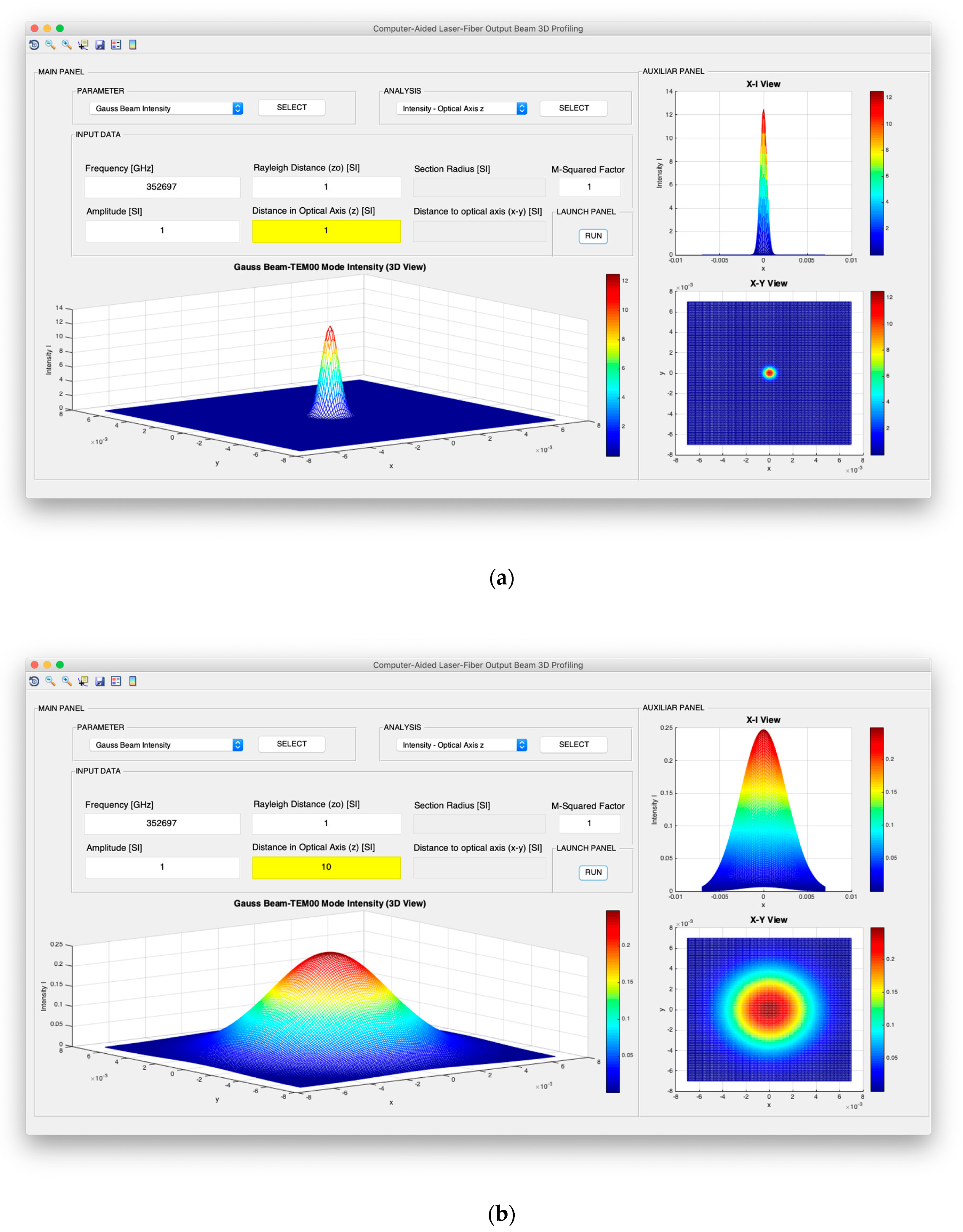
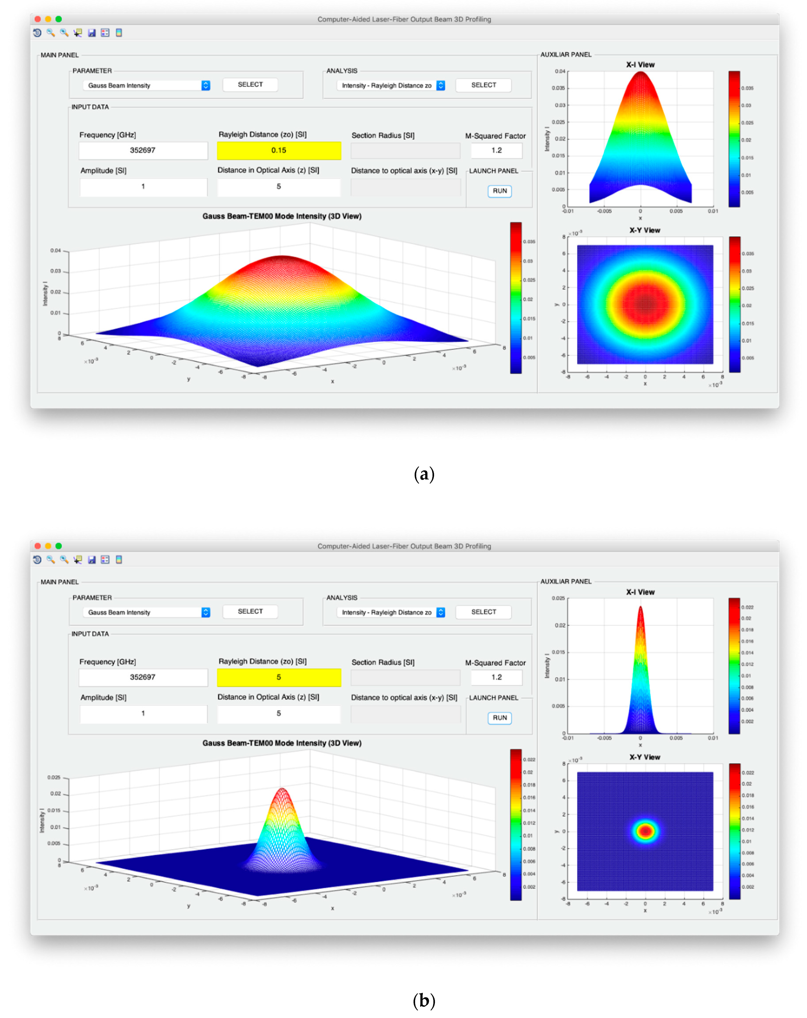
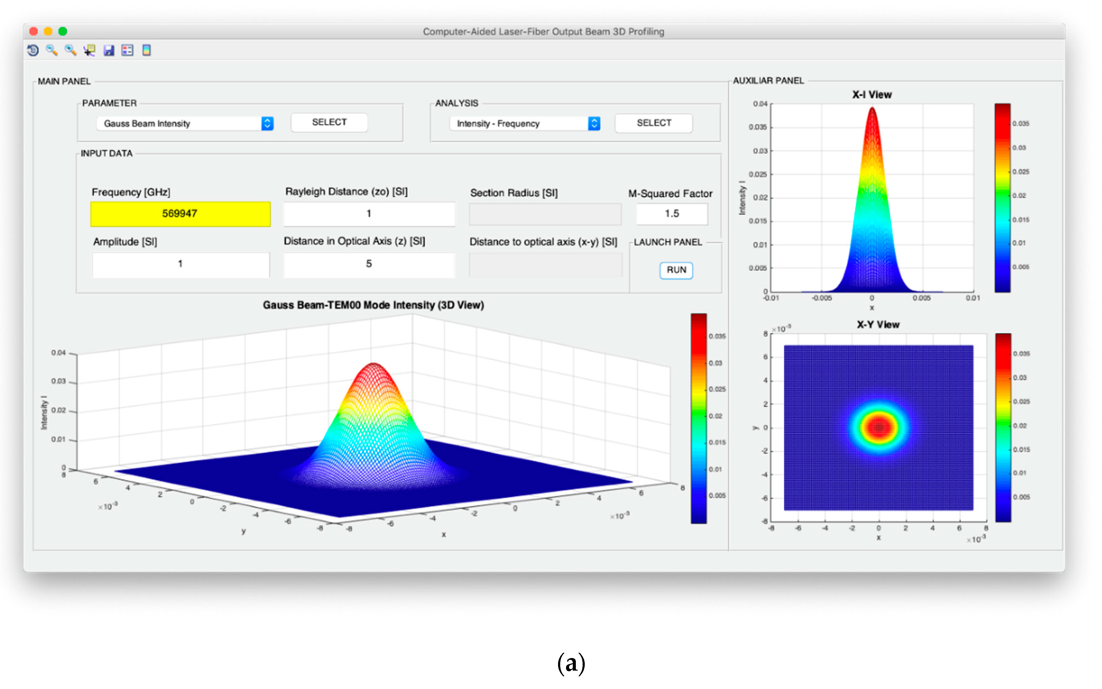
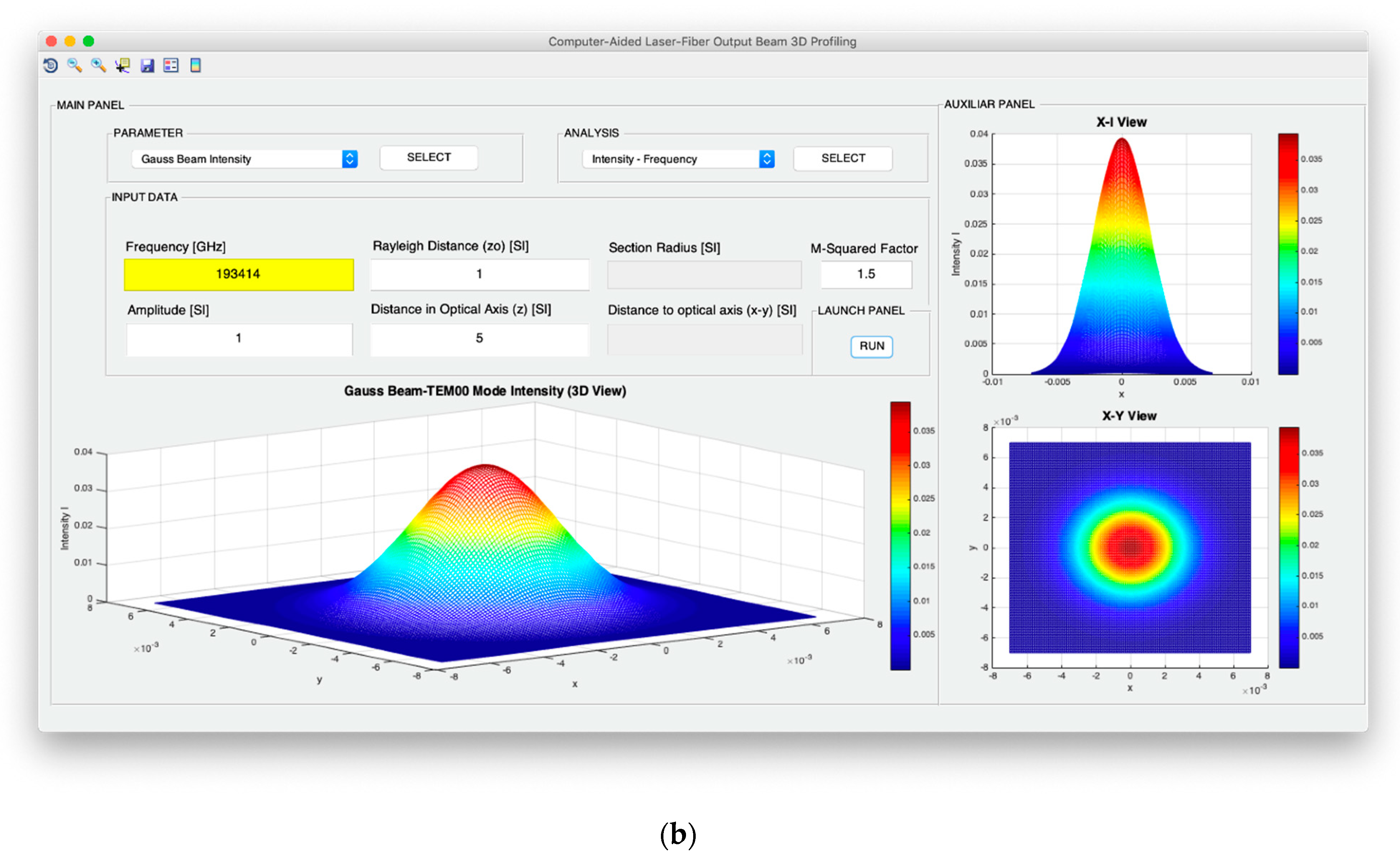
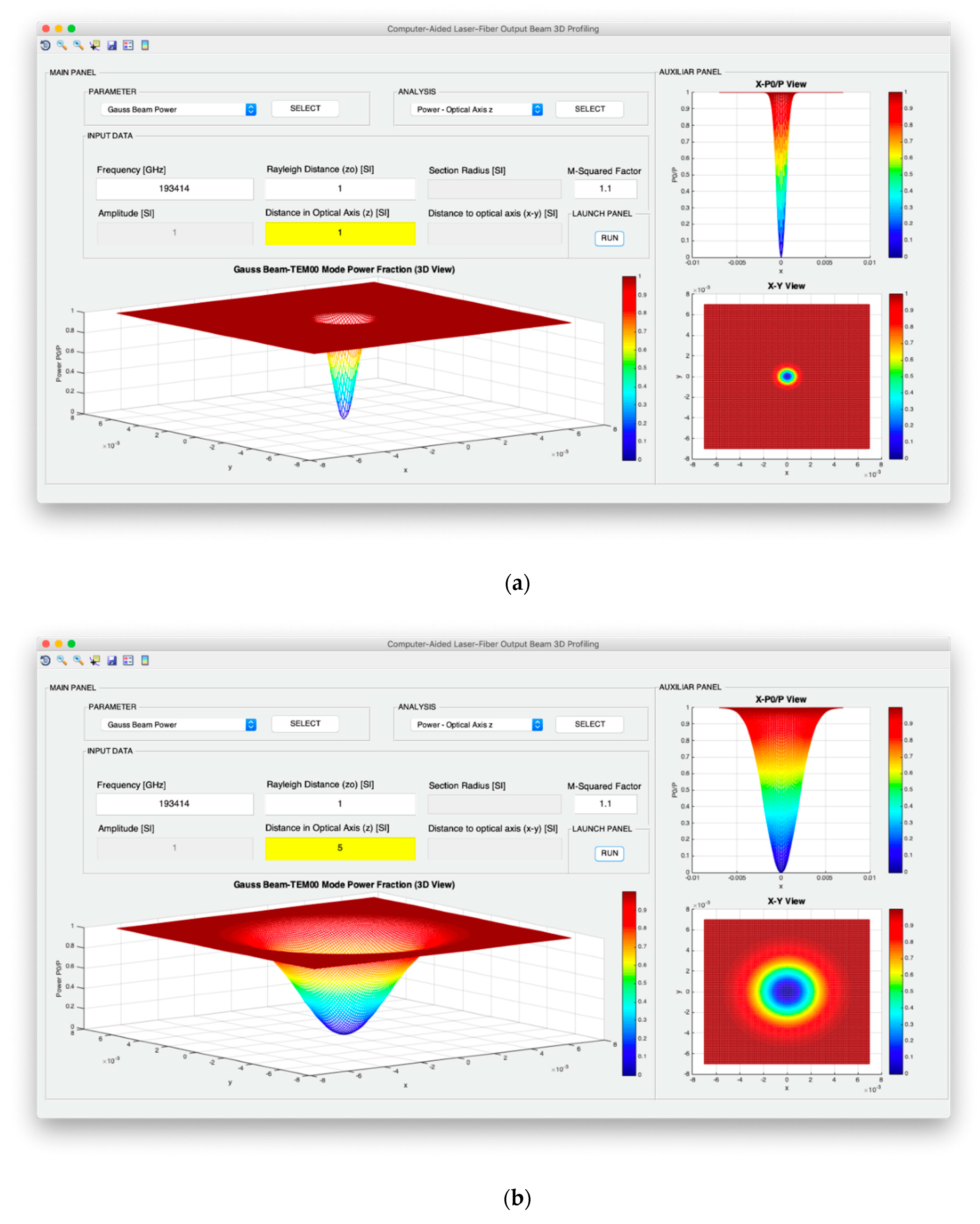
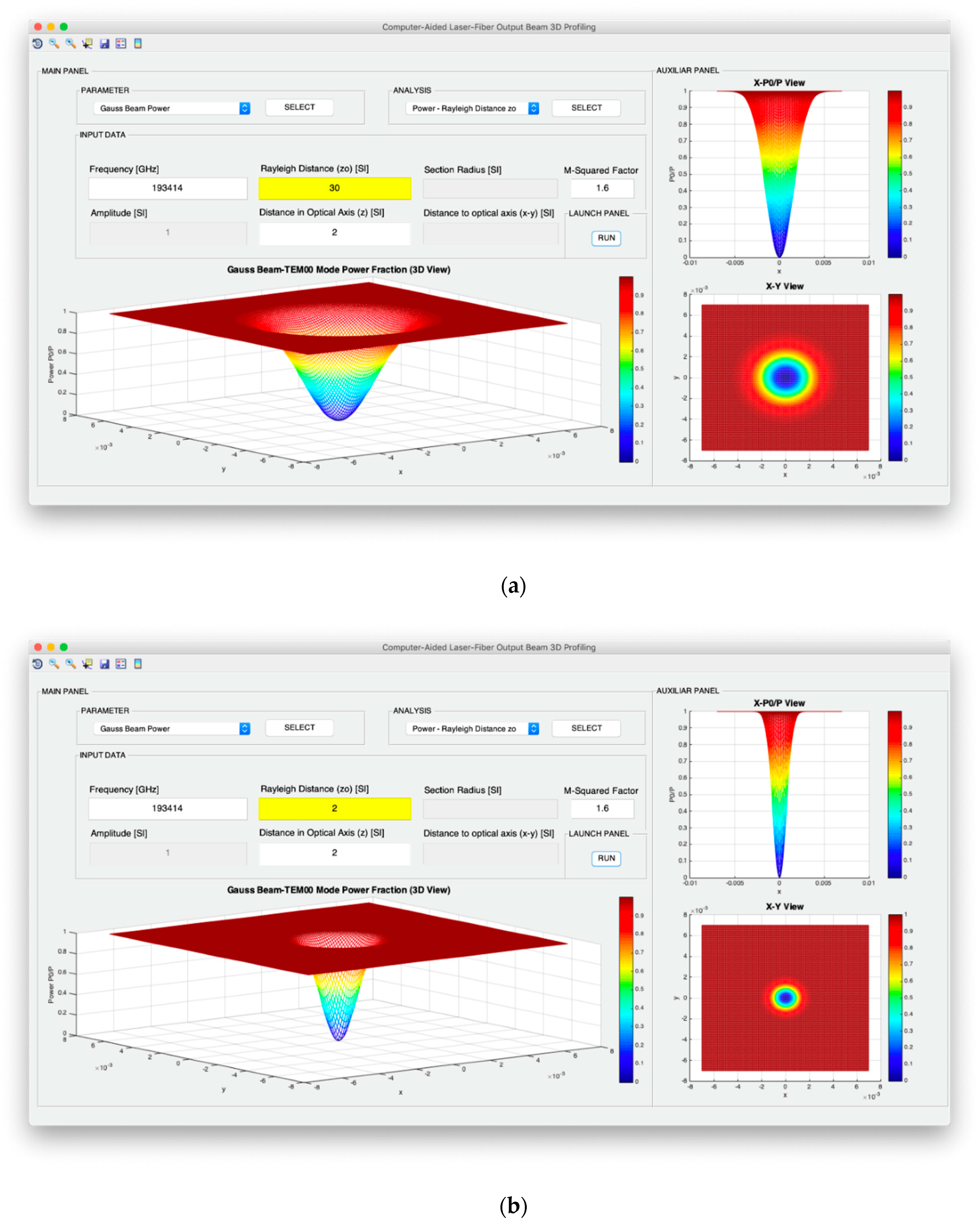
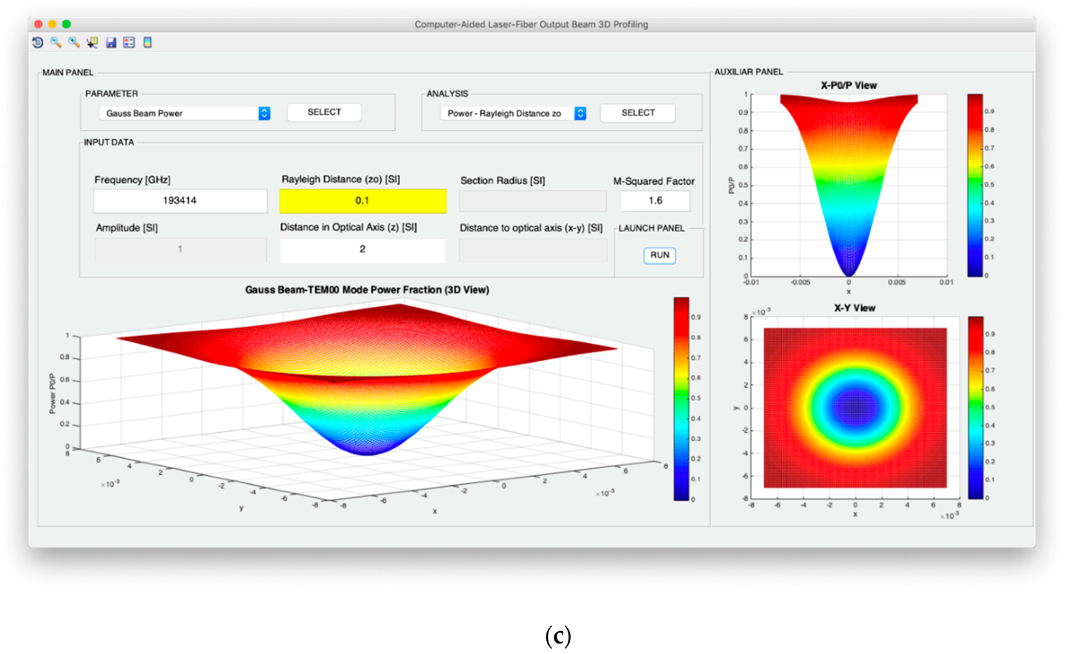
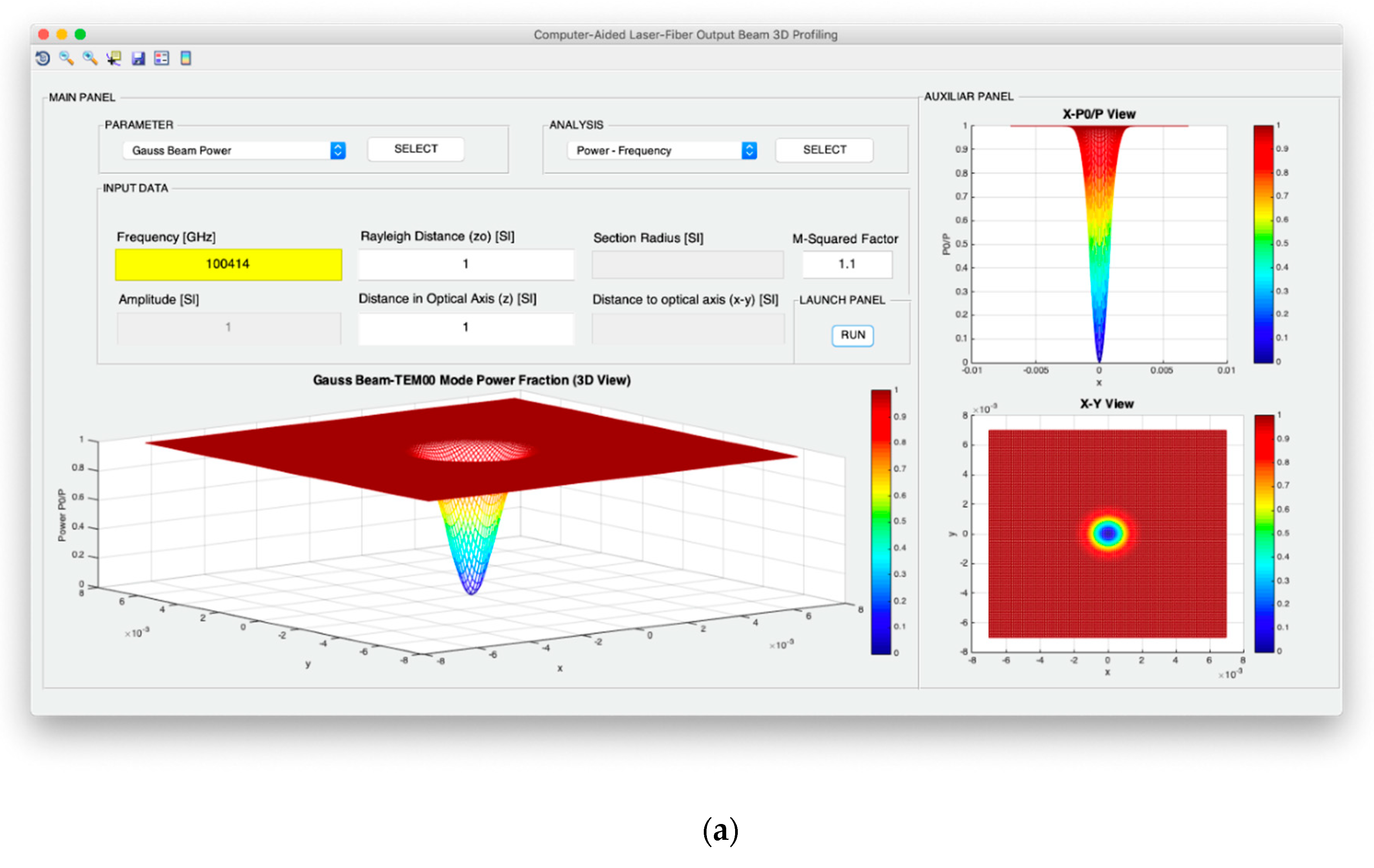
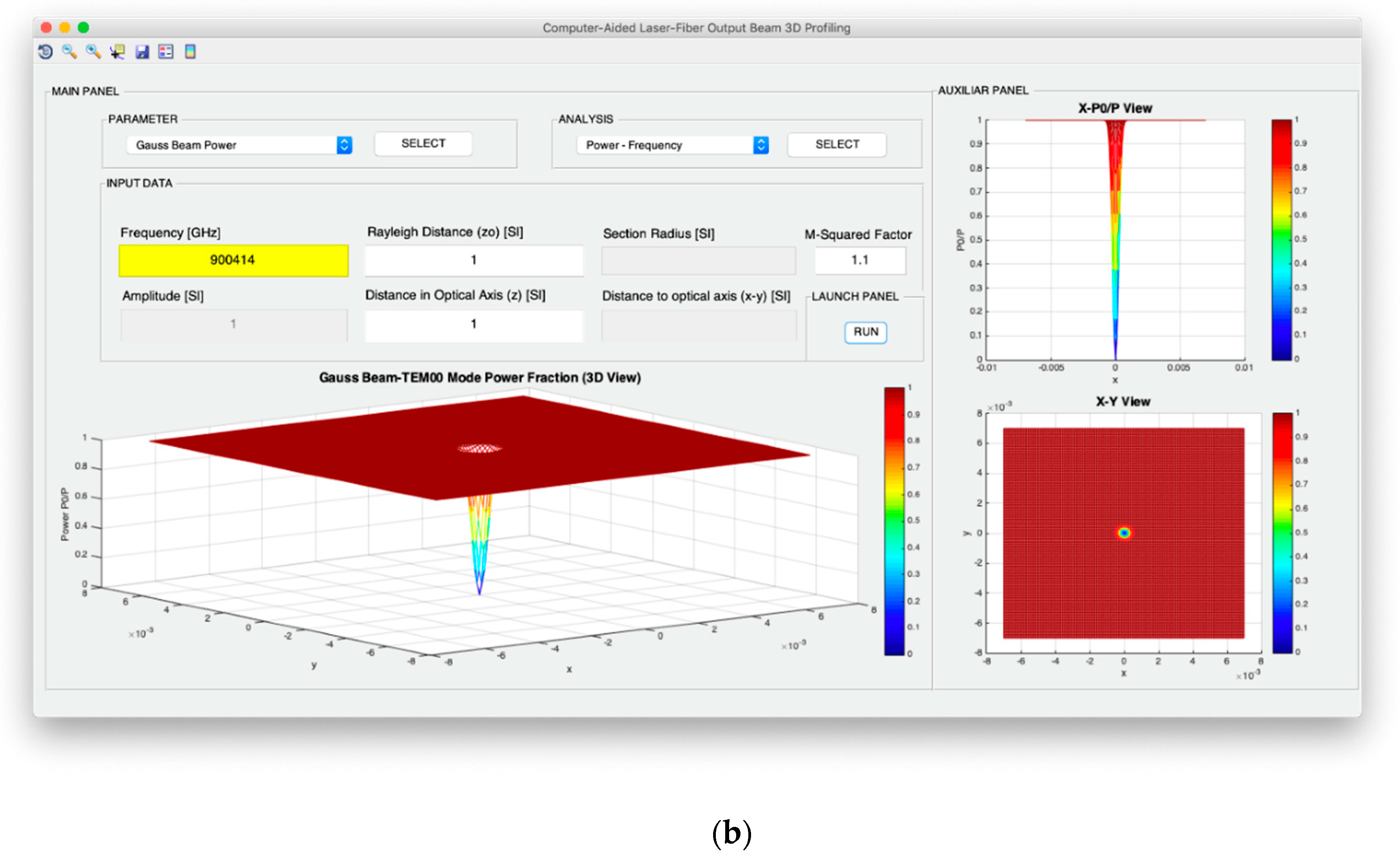
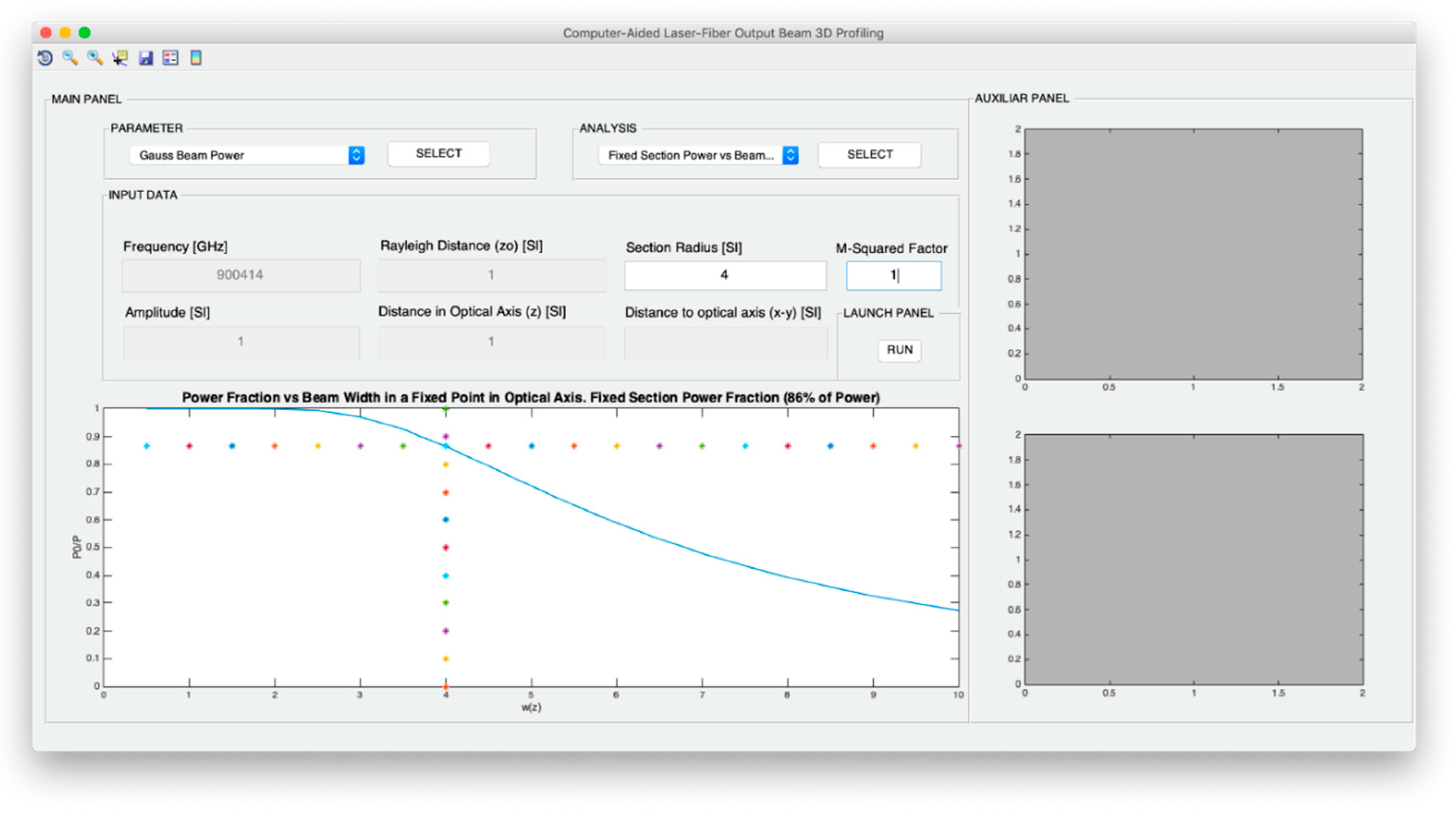
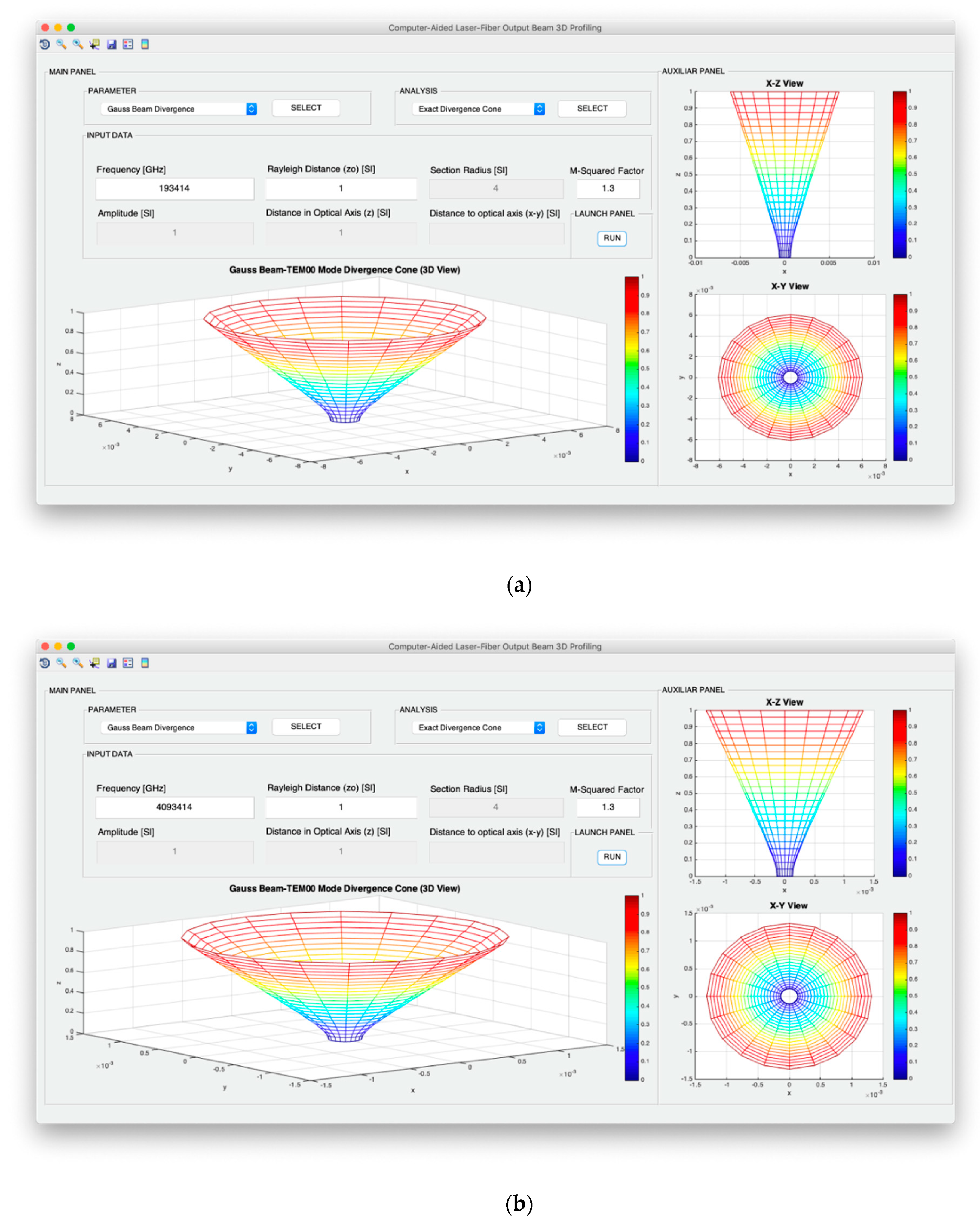
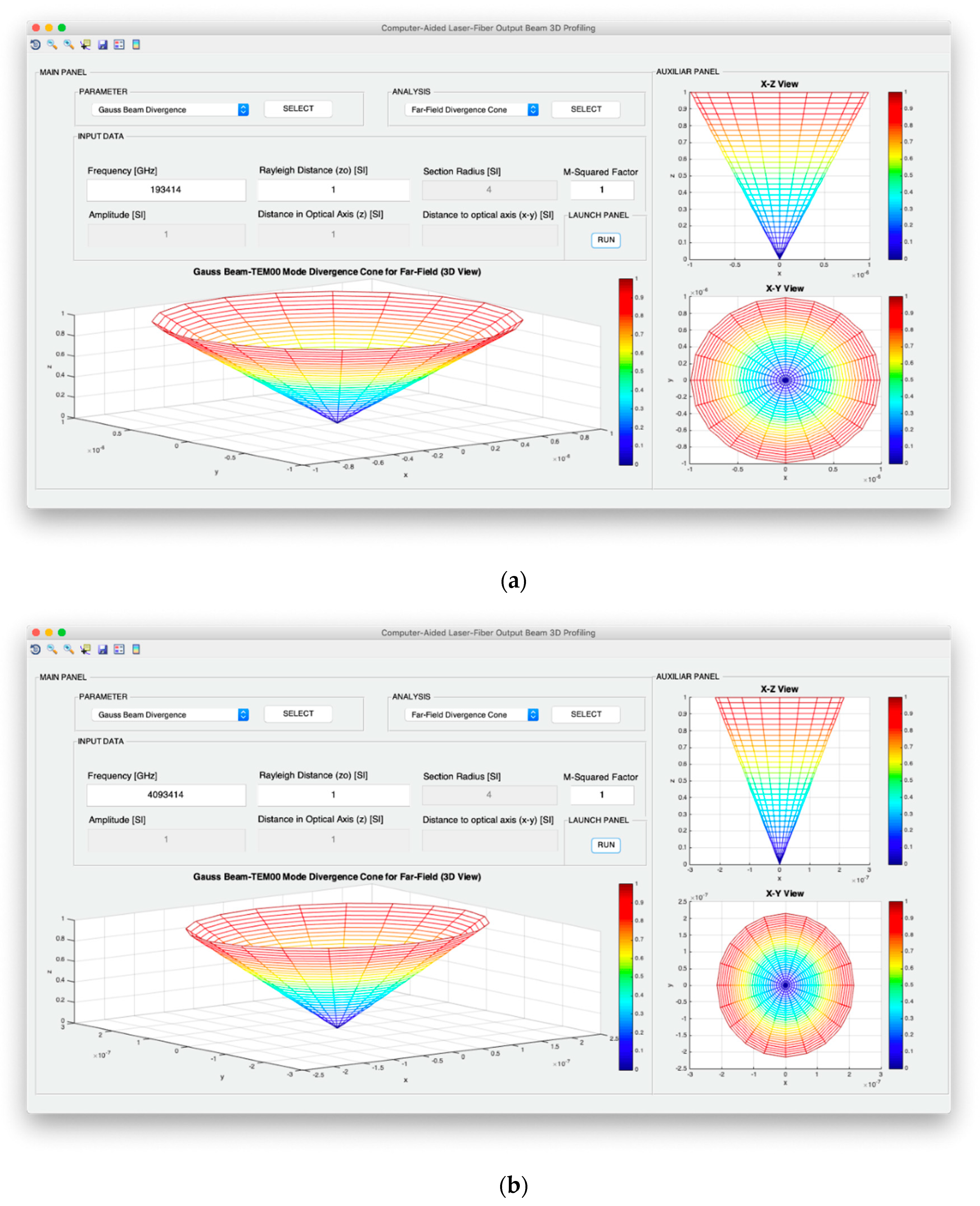
Both intensity and power of TEM₀₀ beams are analyzed from the point of view of the evolution of the optical axis distance, the Rayleigh distance and the frequency of the light source. In addition, for the intensity configuration, the possibility to study the variation in the optical axis of the maximum intensity in consideration not only of the exact expression, but also of the far-field version, is included. Moreover, in the case of the design of the optical power, it is possible to analyze the evolution of the power fraction against the width of the Gaussian beam and obtain said power fraction in a fixed section whose radius coincides with the selected width. In relation to the divergence, the computer profiling system allows modeling the divergence cone of the TEM₀₀ mode considering both its general version and its useful far-field version. The exact divergence and far-field cones are represented by performing the revolution symmetry around the optical axis of the Gaussian beam width and the divergence parameter, respectively.

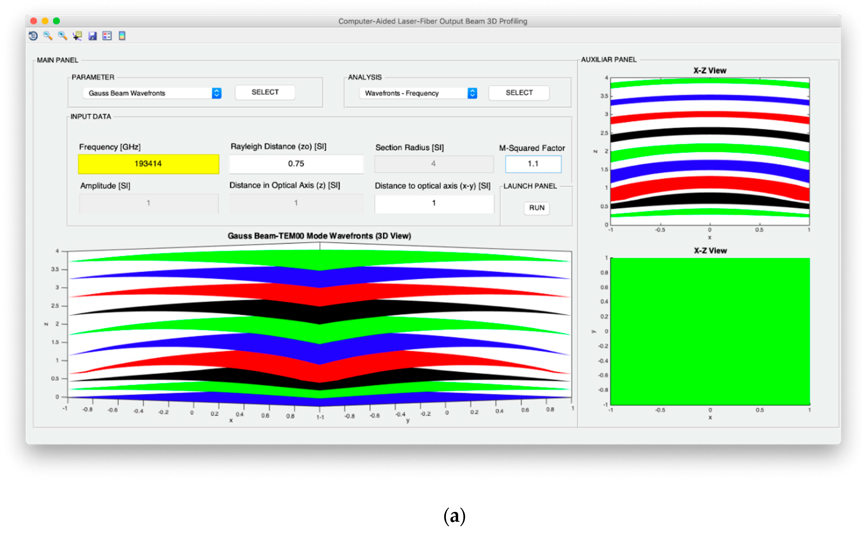
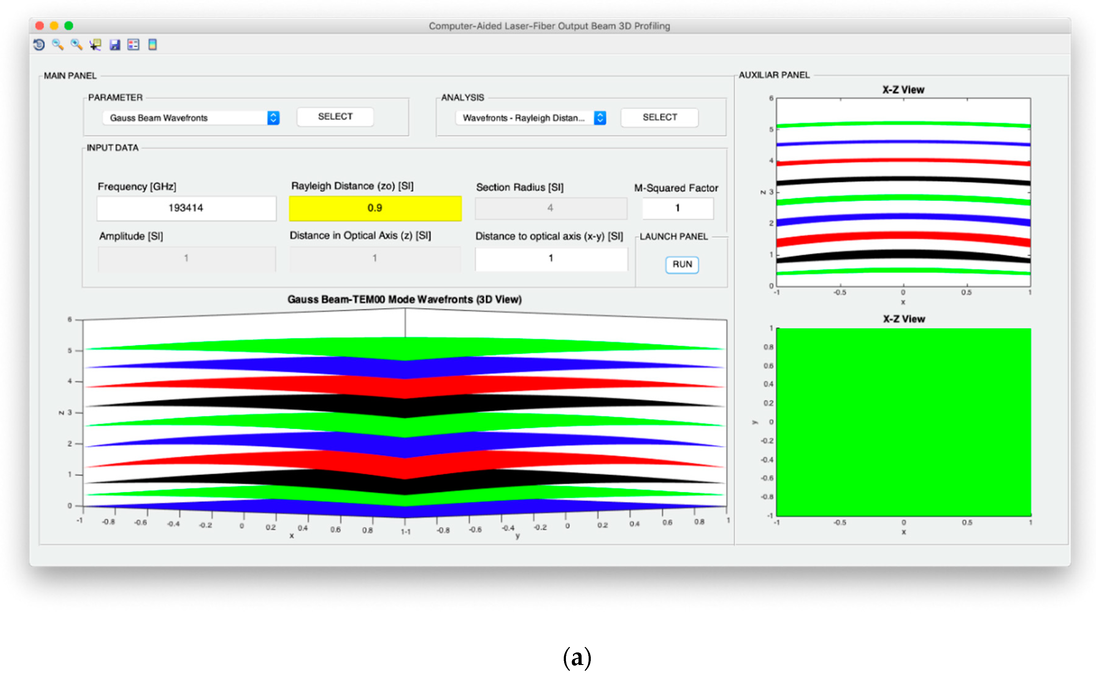
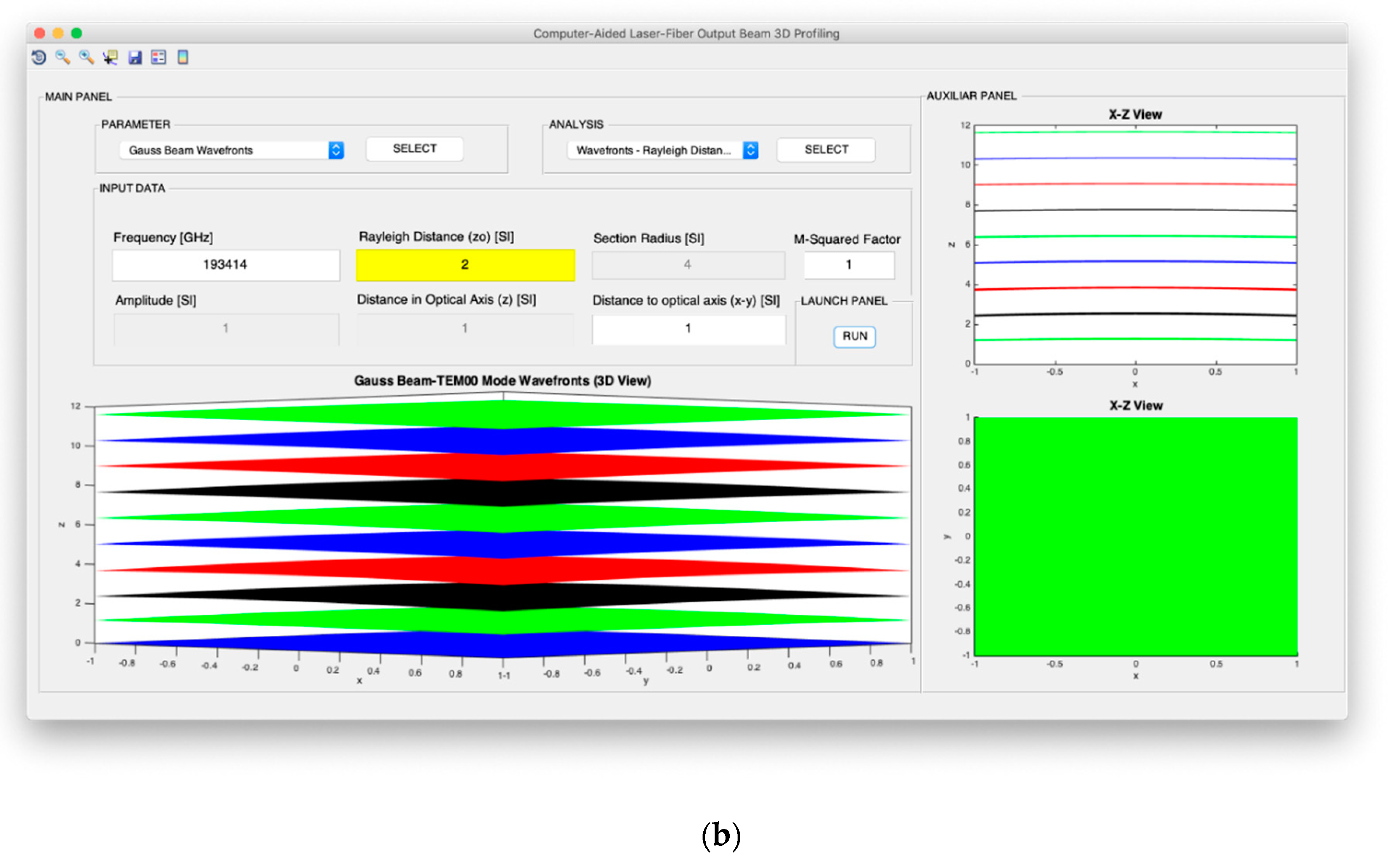
On the other hand, for the design of the angular confinement, the wave fronts of the TEM₀₀ mode are profiled from the point of view of Rayleigh distance to the optical source and the frequency of light emission. It is important to note that the design of the wave fronts must respect the paraxial approach of the Gaussian beam to ensure the validity of the modeling. Finally, as a way of introducing the modeling of the TEM₀₀ and comparative mode in terms of spatial and angular confinement, a section is proposed within the flat and spherical wave characterization design system. 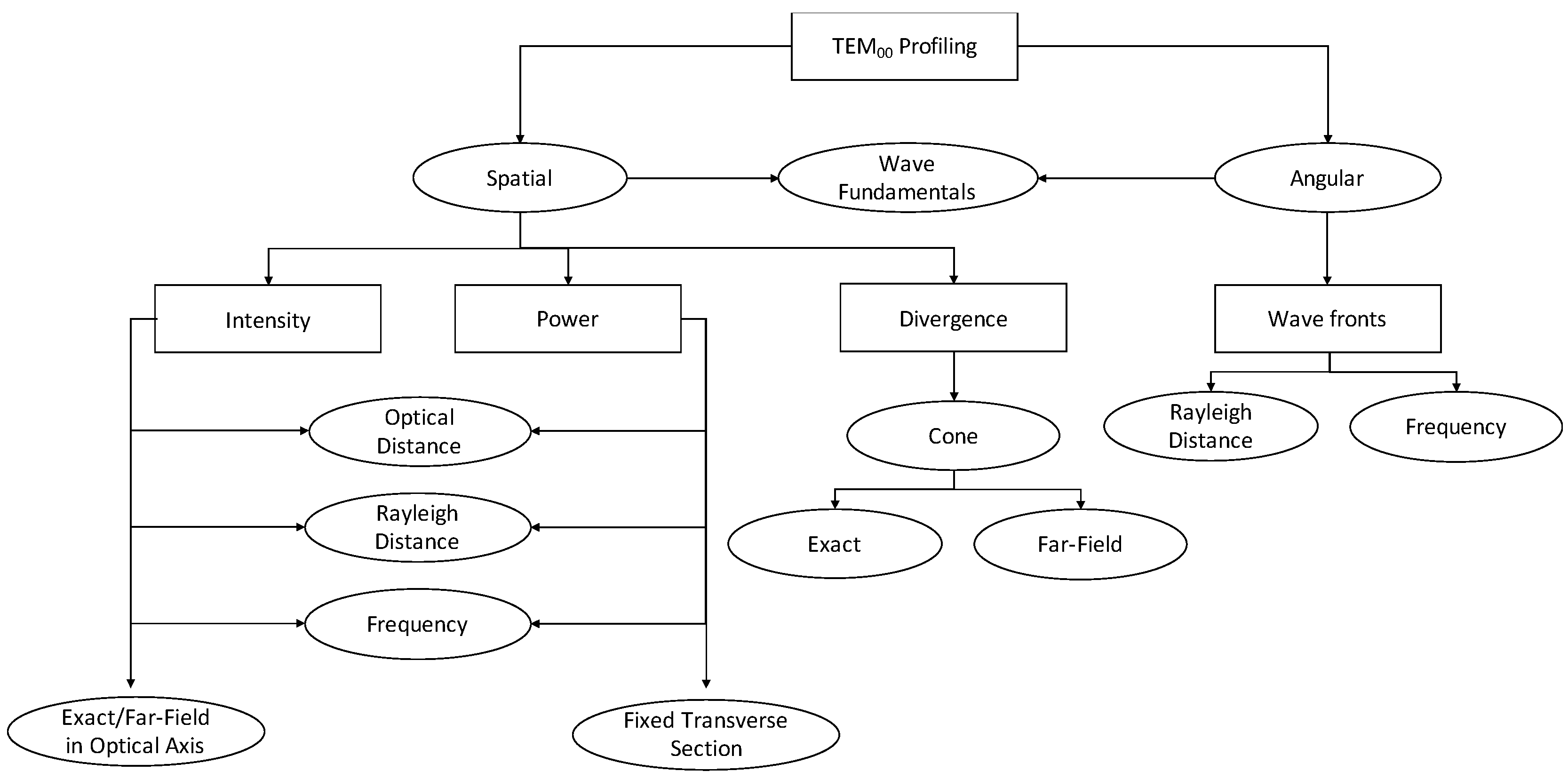Figure 3 shows the scheme of the design areas of the computer-assisted profiler.

Furthermore, Figure 4 shows the flow chart of the operation of the presented tool CATEM00. First, to carry out the design, it is necessary to specify the parameter to be optimized, i.e., the spatial characterization parameter: intensity, power. or divergence, and angular characterization parameter, i.e., the wave fronts or the study of fundamental waves. Once the parameter/study to be analyzed has been selected, the input information must be entered into the design tool. This information includes the frequency, the amplitude, the Rayleigh distance, the distance in the optical axis, the radius of the fixed section and the distance around the x-y axes where it is desired to carry out the paraxial approximation for angular confinement. Once the input information has been entered correctly in format, the beam designer can be executed and the obtained TEM₀₀ beam profile can be observed. If no further analysis of the beam is desired, the tool allows to re-design based on either the selection of the parameter to be designed, the desired analysis or the introduction of parameters for the current design. In addition, it is possible to save the obtained design including the graphic results and the analyzed parameter, the selected analysis and the specific input data. Additionally, the tool provides a more detailed characterization of the obtained results, allowing a rotation of the 3D profile in distance, azimuth and elevation and extracting qualitative data from any point of the graphs, inserting legends or intensity bars to allow a better visual compression of the strength or intensity of the parameter in every point. In addition, after each detailed design analysis, the tool allows one to perform a new analysis, to save the data, or to increase the current results’ analysis.

3.2. Graphical User Interface

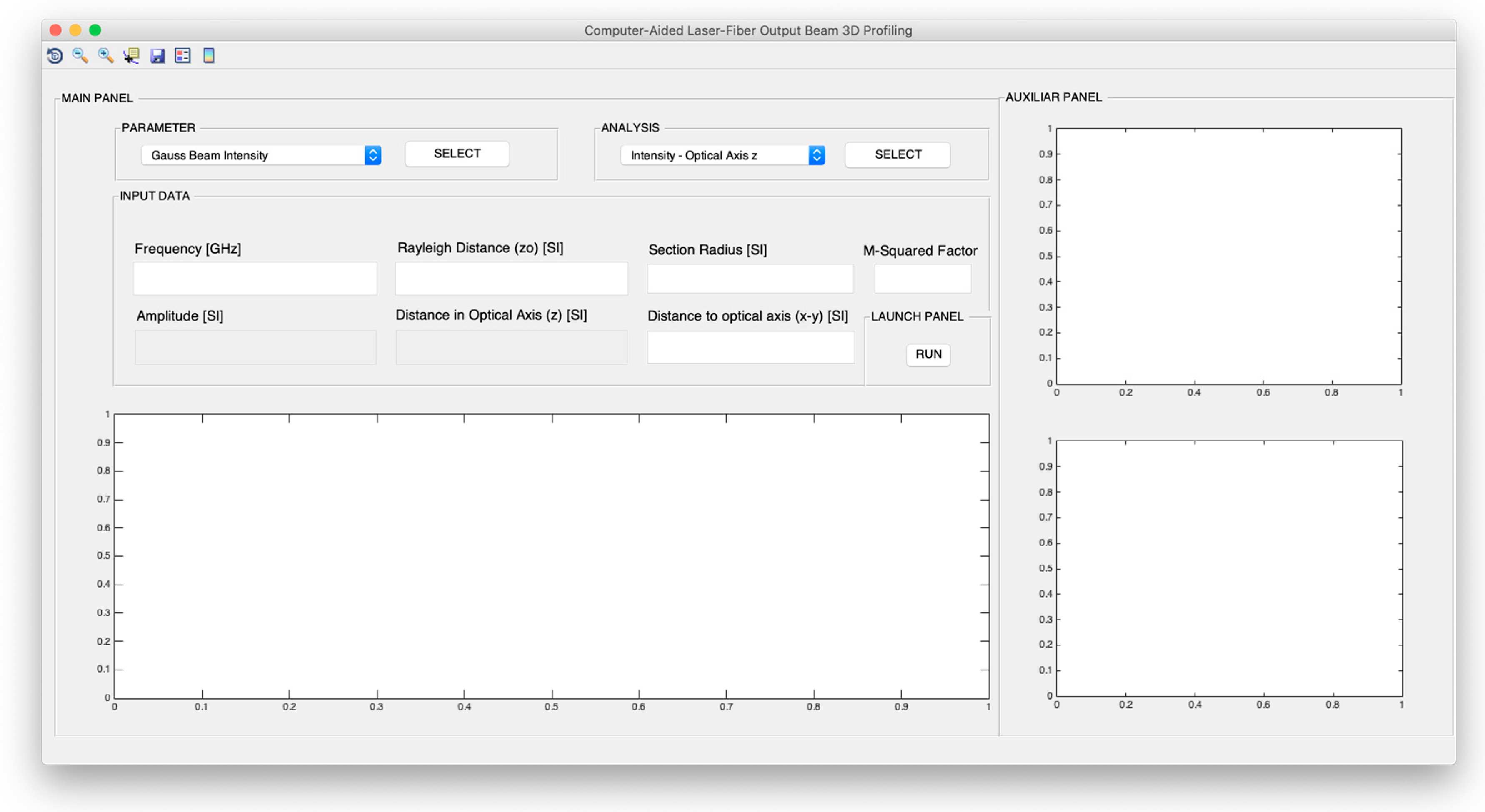
The beam designer is integrated into a graphical user interface to allow greater ease of use of the tool and interpretation of results. As Figure 5 shows, this interface consists of two fundamental panels. On the one hand, the main panel integrates the parameters’ selection, analysis, input, execution, main visualization and, on the other hand, the auxiliary panel allows the plan and elevation visualization of the main visualization. The visualization in plan and elevation is the default configuration that is given to the 3D representations, although it is also possible to configure the desired visualization dynamically by means of the in-depth analysis options of the tool. In addition, as can be seen in the upper left corner of the graphic interface, there is a tool menu for the detailed analysis of the results.

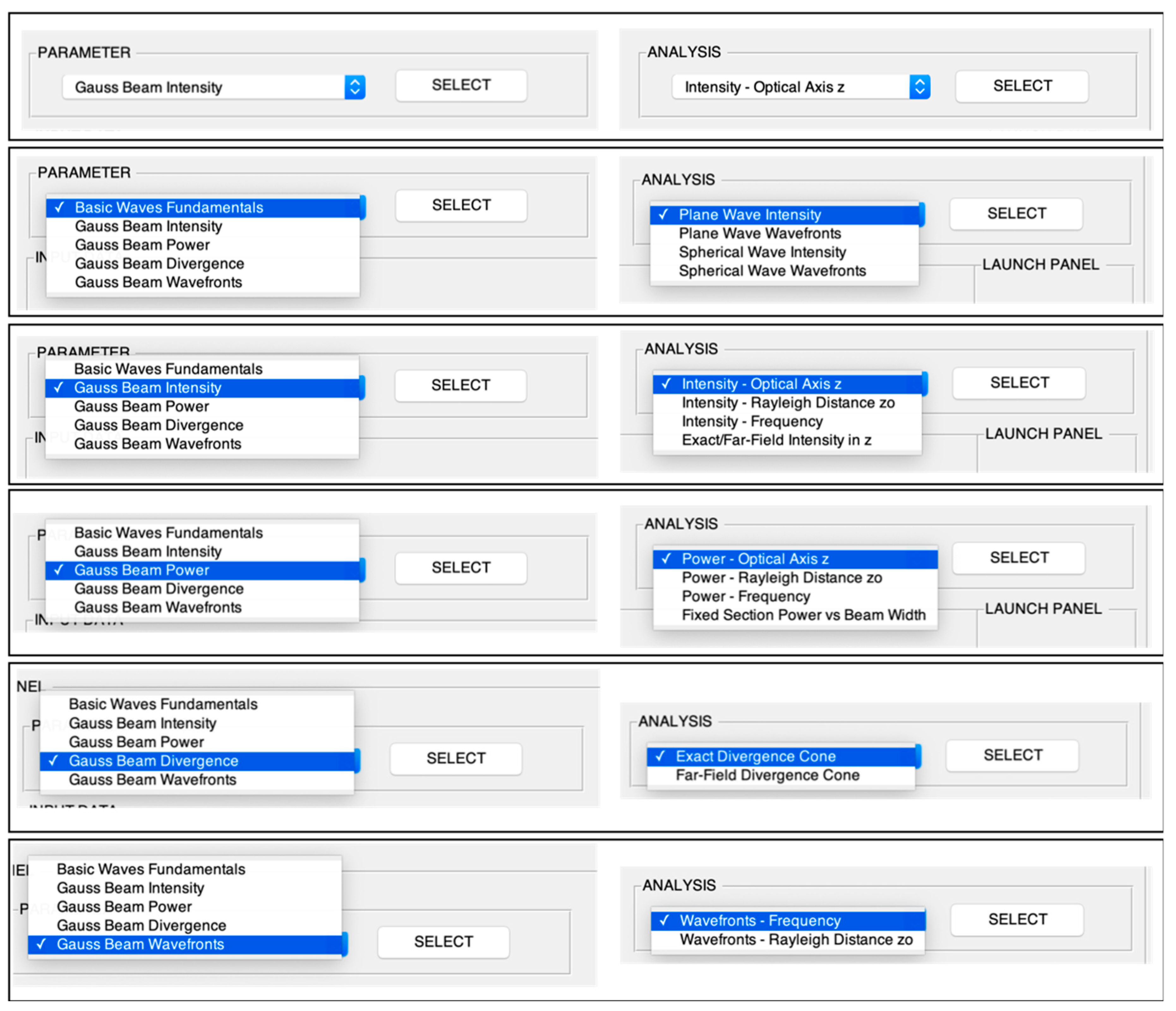
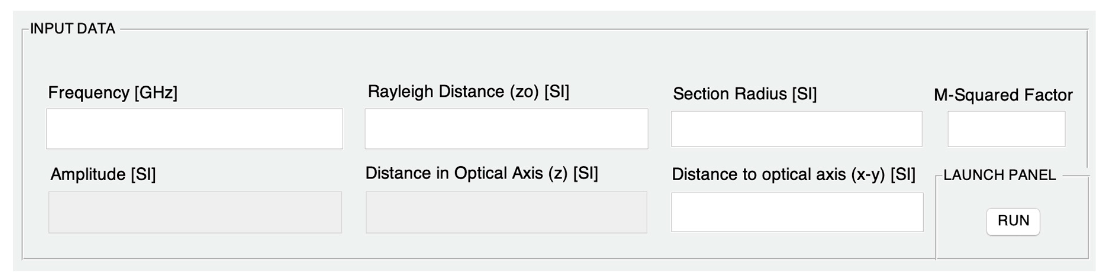
Figure 6 illustrates the parameter selection and analysis panels with all available options. As it can be observed, each parameter study is associated with various options in the analysis panel including all the choices specified in Figure 3 regarding intensity, power, divergence, and wave fronts. Thus, in total, the spatial and angular beam designer allows working with 16 profiling options. Additionally, Figure 7 shows the data entry panel that, as introduced in the previous section, is composed of the information: frequency, amplitude, Rayleigh distance, distance on the optical axis, the radius of the fixed section, the distance around the x–y axes, and the M² factor. It should be noted that, depending on the type of parameter and beam analysis to be designed, the tool automatically enables those parameters and, furthermore, the factor that must be adjusted successively to achieve optimization is highlighted. The launch panel for the execution of CATEM00 is also shown in Figure 7.

4. Results and Discussion

4.1. Intensity Design

As explained, the TEM₀₀ profiler allows the profiling of Gaussian beam intensity in four different aspects. The first characterization is the relation of the intensity with the distance to the light source or optical axis location z. In Figure 8, it can be appreciated the output of the profiler for the Gaussian beam intensity in two different positions of the optical axis (1 m and 10 m) considering the Rayleigh range and the frequency fixed. As observed, as the light advances in the optical z-axis, the Gaussian beam decreases its focality, i.e., light is spread, corresponding to an increment in the beam with W(z). As a function of the distance to the optical axis ρ = (x² + y²)^1/2 it can also be visualized that for each value of z, the intensity depends on the radial distance ρ.

In ρ = 0 (z axis), the intensity reaches its maximum and it decreases as ρ increases. Furthermore, it can be analyzed that this spreading effect is wider as the beam separates from the light source. It is important to realize that W(z) increases when advancing in the optical axis z and so does the intensity spreading along the transverse radio (as pointed out above, the definition of W(z), Equation (6), is related to the intensity spreading).

Additionally, the proposed Gaussian beam profiler allows the simulation and study of the intensity in relation to the depth of the focus (2z₀) or Rayleigh distance (z₀) of the light source. Figure 9 presents three outputs of the proposed profiler, representing the Gaussian beam intensity in a fixed position of the beam axis and a fixed frequency varying the Rayleigh range (0.15 m, 5 m, and 80 m). It can be studied that if z₀ decreases or increases from the considered distance in the optical z-axis, the focality of the light source is decreased, which means that the resulting Gaussian beam intensity profile is the narrowest when z₀ = z. Hence, in z₀ the highest focality is achieved for the TEM₀₀ mode.

Moreover, the Gaussian beam intensity in a fixed position of the beam axis and for a given Rayleigh range varying the frequency can be analyzed with the TEM₀₀ beam profiler. As observed in Figure 10, if the frequency increases, the intensity profile gets narrower, which means that if the frequency is higher, the intensity is more confined around the optical axis. From the definition of the beam waist or spot size of the light source (Equation (7)), the focality (related to depth of focus, 2z₀) becomes greater when W₀ (half of the spot size) increases or when wavelength decreases (increment in frequency value).

Furthermore, the Gaussian beam intensity in the beam axis z considering a given frequency and Rayleigh range against a wide range of distance values z (2D representation) can be obtained with CATEM00. The representation contains a marker point indicating the Rayleigh range and include the approximate intensity or trend that the Gaussian beam intensity follows for far-field conditions (typically 10 times the Rayleigh range).

On the one hand, the exact intensity in the axis corresponds to Equation (11) when ρ = 0:

$$I(0,z)=I_0{\left[\frac{W_0}{W(z)}\right]}^2=\frac{I_0}{1+{\left(z/z_0\right)}^2}$$

(32)

As studied, the Gaussian beam intensity is a function of the distance to the optical axis ρ = (x² + y²)^1/2. Hence, from Equation (32), it can be deduced that the intensity in the z axis ρ = 0 reaches its maximum when z = 0:

$$\max [I(\rho ,z)]=I(0,0)=I_0$$

(33)

and it decays as z increases, reaching half of the maximum intensity value at the Rayleigh range z = z₀:

$$I(0,z_0)=\frac{I_0}{2}$$

(34)

Figure 11 shows that the beam intensity at points in the beam axis (ρ = 0) decreases gradually as the distance to the focus increases, reaching half its peak value at z = ±z₀. It can also be appreciated that the overall peak intensity I(0,0) = I₀ occurs at the beam center (z = 0 and ρ = 0). On the other hand, the approximate expression for intensity in far-field corresponds to:

$$I(0,z)=I_0{\left[\frac{W_0}{W(z)}\right]}^2=\frac{I_0}{1+{\left(z/z_0\right)}^2}\approx I_0{z}_0^2/z^2:z>>z_0$$

(35)

Thus, it can be visualized that the intensity decreases with the distance following an inverse-square law in far-field conditions.

4.2. Power Design

It can be deduced from Equation (13) that the Gaussian beam total power is independent of z (in the absence of attenuation factors) and it corresponds to half of the maximum intensity multiplied by the beam area in the waist position. Nevertheless, a key aspect in the Gaussian beam power analysis resides in its spatial confinement as it propagates along the optical axis. The spatial confinement of the power of the Gaussian beam can be studied with the CATEM00 regarding its relation to the optical distance in z, the Rayleigh distance, and the frequency, as also considered previously for the intensity.

Figure 12 shows the power fraction in the laser position for all x and y directions for different positions in the z-axis and fixed values for the Rayleigh range and the frequency. As observed, the profiler indicates the power circular sections (described by its radius from the optical axis) that contain the diverse power fractions (e.g., power fraction equivalent to 1), and it can be appreciated that the associated radius increases as the Gaussian beam is studied in farther distances from the light source for all the power fractions.

A similar conclusion can be derived from the study of the power fraction in the light source position for all x and y directions for different values for the Rayleigh range and fixed frequency and position in the optical axis, given by the computer-aided tool. As illustrated in Figure 13, the power fraction confined in a fixed section area increases or decreases depending on the fact that the Rayleigh distance is higher or lower than the considered distance in z, achieving the highest spatial confinement when z₀ = z.

Additionally, Figure 14 shows the performance of CATEM00 in the analysis of the power fraction in relation to the frequency. Specifically, the power fraction in the laser position for all x and y coordinates (wide range) for different values for the frequency and fixed Rayleigh distance and position in the optical axis is studied. It can be inferred that, analogously, to the previous intensity versus frequency analysis, the higher the frequency is, the higher the power fraction contained in a predefined section.

Moreover, from the computer-aided profiler it can be deduced that when the considered circular transverse section radius is ρ₀ = W(z) and ρ₀ = 1.5W(z), the contained power is approximately 86.47% and 99%, respectively. Figure 15 shows the power fraction for different values of the beam width W(z). A graphical indication of the power fraction that corresponds to a beam width equal to a selected cross-section is also presented.

4.3. Divergence Design

Regarding the divergence analysis, the beam profiler offers the possibility to study the exact divergence cone and the divergence cone in far-field conditions. Firstly, Figure 16 shows the exact divergence cone for different frequencies values. As known, the exact divergence cone is obtained by the revolution symmetry of the beam width W(z), given by Equation (6), and it contains 86.47% of the emitted power by the light source, approximately. Considering this expression, it can be deduced that the exact divergence cone gets narrower as the frequency is increased.

Secondly, as it can be appreciated in Figure 17, the profiler can also feature the approximate divergence cone for far-field conditions. In this approximation, given by Equation (16), the divergence increases linearly with z, defining a cone with half angle ${\theta }_0$ that approximately contains 86.74% of the power. As observed, the divergence is directly proportional to the relation $\frac{\lambda }{2W_0}$, from which it can be deduced that in order to obtain very directional beams, short wavelengths, or large spot sizes are necessary. Thus, as it can be appreciated in Figure 17 that the higher the frequency (i.e., shorter wavelengths), the lower divergence. Analogous conclusions can be obtained from the analysis of the depth of focus with the proposed tool. The depth of the focus is proportional to the beam area at the light source location and it is inversely proportional to the wavelength, as introduced in Equation (17). Hence, a large depth of focus, or high spatial confinement of light along the z-axis, requires large spot sizes or short wavelengths.

4.4. Wave Fronts Design

Finally, the TEM₀₀ profiler allows the characterization of the angular confinement. In this sense, it has to be remembered here that the Gaussian beam model is founded on the paraxial approximation and so, it is only valid when the wave fronts are tilted less than 30° approximately from the axis beam. This is translated to the fact that the TEM₀₀ wave fronts given by the Gaussian beam model is precise when the beam waist W₀ is larger than 2λ/π, or equivalently, for the radius to the optical source much greater than z, specified by the paraxial approximation of waves. Hence, the presented tool offers the possibility to change the distance to the optical axis, to set up the visualization of the wave front model respecting the paraxial approximation. Equation (19) determines the surfaces of the TEM₀₀ wave fronts, where the radius of curvature R(z) of the wave fronts of a Gaussian beam helps in the analysis of the angular confinement. On the one hand, in z = 0, R(z) = ∞, which corresponds to the radius of curvature of plane wave fronts. On the other hand, in z = ∞, R(z) = z, which corresponds to the radius of curvature of spherical wave fronts that, considering the paraxial approximation, is associated to plane waves in far-field. Finally, in z = z₀, the minimum radius of curvature, or equivalently, the greater angular confinement, is achieved, and this radius corresponds to the spot size, i.e., R(z) = R_min = 2z₀. Figure 18 shows the output of the computer-aided profiler for wave fronts considering different values for the frequency, confirming the previous analysis. It can be appreciated that the greater the frequency is, the lower the curvature radius of the wave fronts and, so, the greater the tilt of the wave fronts.

Moreover, CATEM00 allows the analysis of the dependence of the TEM₀₀ wave fronts and the Rayleigh range z₀. Figure 19 depicts the output for the wave fronts for two different Rayleigh distances, where it can be inferred that the higher the Rayleigh distance, the greater the achieved angular confinement. That is, the normal vectors to the wave fronts form smaller angles with the optical axis-z along z.

5. Conclusions

The proposed computer-aided TEM₀₀ beam tool CATEM00 provides a complete and freely-available solution for the visual design in 3D of multiple lasers and single-mode fiber output beam. Based on the fundamentals of Gaussian beam propagation in wave theory, the design is possible not only in the characterization of the associated light sources in relation to their spatial confinement, considering intensity, power, and divergence, but also in relation to its angular confinement, in the form of limited wave fronts according to the paraxial approximation. It should be noted that both the design and the knowledge of the dependence of the beams, both in space and at an angle, make it possible to propose and detect the quality of the beam with precision, which is very critical in various applications, especially in biomedical related to surgery [1]. The tool has been developed in MATLAB code and the support platform for its execution is provided free of charge, in a way that the distribution of the work can be extensive. In addition, the graphical user interface that integrates the designer makes the propagation details transparent and allows simple modeling based on the characteristic parameters of Rayleigh range, amplitude, distance on the optical axis z, radial distance to the optical axis z, and radius of the fixed section to be considered. Finally, all the necessary quantitative values can be obtained from the configurable graphic displays in azimuth, elevation, and distance. In future works, the integration of further transversal modes of light sources and lenses will be considered. Moreover, the tool will be also offered in other programming languages to make it as accessible as possible to the scientific community.