PointNet++ and Three Layers of Features Fusion for Occlusion Three-Dimensional Ear Recognition Based on One Sample per Person

Abstract

The ear’s relatively stable structure makes it suitable for recognition. In common identification applications, only one sample per person (OSPP) is registered in a gallery; consequently, effectively training deep-learning-based ear recognition approach is difficult. The state-of-the-art (SOA) 3D ear recognition using the OSPP approach bottlenecks when large occluding objects are close to the ear. Hence, we propose a system that combines PointNet++ and three layers of features that are capable of extracting rich identification information from a 3D ear. Our goal is to correctly recognize a 3D ear affected by a large nearby occlusion using one sample per person (OSPP) registered in a gallery. The system comprises four primary components: (1) segmentation; (2) local and local joint structural (LJS) feature extraction; (3) holistic feature extraction; and (4) fusion. We use PointNet++ for ear segmentation. For local and LJS feature extraction, we propose an LJS feature descriptor–pairwise surface patch cropped using a symmetrical hemisphere cut-structured histogram with an indexed shape (PSPHIS) descriptor. Furthermore, we propose a local and LJS matching engine based on the proposed LJS feature descriptor and SOA surface patch histogram indexed shape (SPHIS) local feature descriptor. For holistic feature extraction, we use a voxelization method for global matching. For the fusion component, we use a weighted fusion method to recognize the 3D ear. The experimental results demonstrate that the proposed system outperforms the SOA normalization-free 3D ear recognition methods using OSPP when the ear surface is influenced by a large nearby occlusion.

1. Introduction

As a body part used for biometric identification, the ear exhibits certain advantages over several other body parts. The ear has permanent structural features that maintain the same shape, and its shape is robust to expression [1]. Clinical observation shows that the shape of the ear is not affected between the ages of 8 and 70 years [2]. Ear recognition can be performed in a non-contact manner. Furthermore, because the ear is located adjacent to the face, it can provide valuable information to supplement facial images. Despite having unique and rich features, establishing robust ear biometrics for practical application with the registration of only one sample per person (OSPP) in the database, such as access control and passport identification, is an arduous task. The three-dimensional (3D) data-based recognition method can eliminate the low performance of the two-dimensional (2D) image-based recognition method because of the variation in illumination and pose. Therefore, we should acquire and use maximum information from a single registered 3D sample per person.

To cope with the OSPP problem, the large occlusion problems must be addressed during the identification procedures. The quality of ear samples is easily affected by large occlusions, such as hair and earrings, between the camera lens and ears. Therefore, only partial data from the probe ear can be utilized during the recognition process. Figure 1 depicts several images of the partially occluded ears. The first image from left to right is an ear image with long-distance object occlusion, whereas the second, third, and fourth images are ear images with short-distance object occlusion. The majority of the existing ear biometrics either exhibit considerably low performances or fail to work with partial data and under OSPP conditions [3], i.e., the per-person registered sample size required for training the majority of the existing ear recognition methods based on deep learning is difficult to satisfy when only OSPP is registered in the gallery [4]. Thus, developing an ear recognition system that can handle partial data problems using OSPP is necessary. The depth information can effectively assist the separation of occlusion from the ear when the occlusion is far from the ear [4]. However, the separation of the ear from the occlusion as well as the extraction and recognition of the ear surface features become challenging when large occlusions are close to the ear. Furthermore, in practical applications, the probe samples are difficult to automatically normalize because of the effect of occlusion. Thus, most ear recognition methods can only exhibit considerably low performances, i.e., deep-learning-based ear recognition method under unconstrained conditions, such as pose variation, is a challenging task when there are insufficient gallery ear samples per person [5,6]. Therefore, in this study, we exclusively focus on normalization-free 3D ear recognition using the OSPP partial data when the large occlusion is close to the ear surface.

Herein, inspired by our previous work [4] and PointNet++ [7], we present a PointNet++, local feature, local joint structural (LJS) feature, and holistic feature fusion based on a fully automatic system for OSPP normalization-free 3D ear recognition when the large occlusion is near the ear surface. This system can be referred to as the PointNet++ and three layers of features fusion (PTLFF) system. The motivations behind combining PointNet++ and three layers of features for 3D ear recognition are as follows. (1) PointNet++ [7] can effectively segment 3D objects with complex shapes affected by partial occlusion from an input 3D scattered point cloud in the clutter scene; thus, it is suitable for robustly segmenting the ear from the input 3D point cloud data. (2) Accurate segmentation of the ear can promote the effective extraction of discriminant features. (3) Local representation has been found to be more robust to clutter and occlusion than LJS and holistic representation [8]. (4) LJS representation captures the relative pose information of two local surface patches, resulting in effectively making up for the limitation of recognition performance caused by the difficulty of using this information in local representation. (5) Holistic representation captures information from the entire segmented surface without excluding any information that describes the ear [8]. (6) The performance of ear recognition can be improved by effectively fusing the aforementioned complementary information. This idea of using multi-layer features is similar to state-of-the-art (SOA) deep-learning-based recognition method.

Figure 2 depicts the architecture of the proposed system. The system comprises four important components: segmentation, local and LJS feature extraction and matching, holistic feature extraction and matching, and fusion. For a given cloud data point, the segmentation component can provide a set of 3D points to represent the ear. For the local and LJS feature extraction and matching component, the data is first preprocessed by fitting the segmented 3D point set by an implicit surface. Then, it is transformed onto the generated implicit surface by calculating the orthogonal projection from 3D points to implicit surfaces. Second, the shape index and curvedness feature of the transformed 3D point is computed using the implicit surface. Third, for keypoint selection, a set of keypoints is extracted from the generated implicit surface at a salient location. Fourth, the local surface patch centered on each keypoint is cropped, and the SOA surface patch histogram indexed shape (SPHIS) local feature descriptor is obtained. Fifth, a local joint structure is presented. This structure comprises two local surface patches centered on two keypoints. Subsequently, a pairwise surface patch cropped using a symmetrical hemisphere cut-structured histogram of indexed shape (PSPHIS) feature descriptor is extracted to encode the LJS information of the ear surface. Sixth, for the local and LJS matching engine, a set of correspondences between each keypoint of the probe ear to five (at most) of its nearest neighboring keypoints of the gallery ear is obtained. Under the symmetrical game theory (GT) pipeline, non-outlier correspondences are detected using transformed 3D points and geometrical and local and LJS information constraints; then, they are utilized to make the associated probe–gallery–ear model pair registration and voxelization. For holistic feature extraction and matching, the registered voxelized ear models are vectorized, and a match score is calculated using the cosine distance between the voxelized representations of the probe–gallery pair. For the fusion component, a weighted fusion strategy is used to fuse two matching scores from both the GT pipeline-based local and LJS matching and voxelized strategy-based holistic feature-matching components.

The remainder of this paper is structured as follows. Section 2 discusses related works. Section 3 applies the automatic segmentation of the ear for a given 3D point cloud of the profile face, and Section 4 details the proposed techniques for the extraction and matching of local and LJS features, including an improved keypoint selection method, a rotation-invariant LJS representation, and a matching engine by combining local and LJS features. Section 5 details the voxelization method for holistic representation. Section 6 details the weighted fusion structure that combines the match scores obtained using the local and LJS matching engines and holistic matching engine. Section 7 presents experiments and further discussions, and Section 8 presents the conclusions of our study.

2. Related Work and Contributions

The human ear can be considered to be an approximate rigid 3D biometric feature comprising abundant structural information that can be used for identification. Several studies have investigated ear biometrics, and good performance has been reported [8,9,10,11,12]. However, as discussed herein, the OSPP, pose variation, and partial data scenario in which the majority of the occlusions are close to the ear surface are common in real-world applications. The majority of the existing automatic ear recognition methods require identification information from multiple training samples in the gallery, normalized data with few outliers, or occlusion at a distance from the ear; furthermore, many existing methods fail to use the 3D depth information of the ear.

Yan and Bowyer [10] presented an ear recognition approach. Initially, they established a fusion method based on the nose tip location, the ear pit location, and an active contour model; they applied this method to segment the ear based on a profile face image. Subsequently, they proposed an ameliorative iterative closest points (ICP) method to match the ears. Chen and Bhanu [11] presented a 3D ear recognition system that can perform ear detection, identification, and verification. They presented a method that used a training ear-shaped model to obtain the position of the ear helix and antihelix components. They proposed ear helix/antihelix and local surface patch representations for ear identification and verification. Cadavid and Abdel-Mottaleb [12] investigated 3D ear biometrics based on uncalibrated video sequences. They used a shape from the shading technique to perform 3D reconstruction of the interest region from a video clip region. Further, they registered these 3D models using the modified ICP technique. Zhou et al. [8] suggested a 3D ear biometric that combined the local and global features. They utilized a surface patch shape descriptor and the iterative orthogonal Procrustes analysis method to calculate the local match score. Furthermore, a surface voxelization method was used to obtain the holistic match score. Sun and Zhao [13] proposed a 3D ear point cloud registration method. They initially extracted the multiscale feature point sets using the scale-invariant feature transform algorithm and subsequently registered feature point sets parallel to their cascaded expectation maximum–iterative closest points (EM–ICP). Ganapathi and Prakash [14] proposed a spin image-based 3D ear recognition approach. They used the geometric properties of the ear surface to eliminate the false corresponding features. Further, Tharewal et al. [15] presented a multimodal biometric technique. They separately recognized the face and ear images and combined the match scores obtained from both the models to generate the final recognition result. Zhang et al. [16] suggested an efficient 3D ear biometric system. Based on a local appearance descriptor, the ear data are normalized and the smooth region is removed, resulting in reduced ear data size for registration. Ganapathi and Prakash [9] also suggested a 3D ear biometric based on the local and holistic features. They proposed a statistical information-based global feature descriptor and a linearized feature combination strategy for recognition. They achieved a rank-1 recognition rate of 98.69% based on the University of Notre Dame Collection-J2 Database.

A GT-based method can completely utilize the superiority of the local descriptors and their mutual spatial position relation because the essence of GT, i.e., the optimization of a candidate strategy set generated via the candidate keypoint correspondence, allows every strategy contained within it to compete with each other in the evolutionary theory framework to maximize the total payoff. This results in a subset of keypoint correspondence associates with a subset of strategy that occupies a large share. The GT-based method can handle the OSPP problem because it obtains matching scores using only the gallery and query samples. Albarelli et al. [17] proposed a non-cooperative GT-based 3D subject classification method. They adopted an evolutionary selection algorithm for extending the property of local descriptors to abide by the pairwise spatial distance constraints. Furthermore, Albarelli et al. [18] suggested a surface registration method through an isometry-enforcing game. A set of point correspondence, which satisfies the joint rigidity constraint, can be obtained from the surface of the objects by implementing a GT framework. Zhu and Mu [4] extended this method using SPHIS and long-distance occlusion-independent SPHIS (LOSPHIS) descriptors to surmount the OSPP challenge in ear recognition. They proposed a two-step non-cooperative game-based (TNG) recognition method. In the first step, a set of keypoint correspondence was obtained from a set of candidate keypoint correspondences in which the $L_2$-norm distance between the two SPHIS descriptors associated with every candidate keypoint correspondence was small, aligning the query and gallery images. Further, in the second step, a set of aligned new keypoint correspondences was acquired. In addition, the difference between the LOSPHIS feature vectors for each keypoint correspondence was observed to be less than the threshold. Each correspondence could not be selected as the candidate keypoint correspondence in the first step of the game, because the corresponding local SPHIS descriptors were affected by large occlusion. However, when the large occlusion was close to the ear, the LOSPHIS feature vectors were difficult to extract, resulting in failure in the second step of the non-cooperative game. Thus, the discriminant ability of the existing GT-based ear biometrics is low when the large occlusion is close to the surface of the probe ear.

The primary contributions of this study are as follows. (1) This paper first proposes an OSPP 3D ear recognition system that integrates the ear segmentation results obtained using PointNet++ and three layer of features without normalized ear data. (2) The experiments denote that the proposed system outperforms the SOA normalization-free OSPP ear recognition method when a large occlusion is present close to the probe ear. (3) A novel local joint structure, referred to as the two-keypoint structure, has been proposed to represent the joint shape of two separated local surface patches. (4) Based on the histogram of the indexed shape (HIS), an LJS descriptor, referred to as a PSPHIS descriptor, is developed for two-keypoint structure description and matching. (5) A local and LJS feature-matching engine is proposed under the GT pipeline to detect non-outlier correspondence between the probe and gallery ear models more effectively. (6) A sphere-based robust keypoint selection method is proposed to select a set of potential keypoints insensitive to data variations.

3. Segmentation

To directly process the set of scattered points, Qi et al. [7] proposed PointNet++. PointNet++ is a hierarchical neural network. The steps involved in feature extraction include the following: local region division of point set, feature representation of fine geometric structure, and the generation of higher level features. To perform the object segmentation task using PointNet++, a hierarchical propagation strategy across level skip links and with distance-based interpolation is selected [7]. Meanwhile, PointNet++ can segment objects with complex shapes in cluttered scenes more accurately. Therefore, PointNet++ was used to segment the ear from the input profile face 3D point cloud.

4. Local and LJS Feature Extraction

The ear segmentation component outputs a set of 3D points representing the ear. The next component involves extracting and matching local and LJS features. This component comprises six subtasks: data preprocessing, shape index and curvature feature calculation, keypoint selection, local feature extraction, LJS feature extraction, and a matching engine of local and LJS features.

4.1. Data Preprocessing

Previous studies have shown that the efficient calculation of the principal curvature of 3D points on implicit surfaces [19] can efficiently extract SOA SPHIS local feature descriptors [12]. Therefore, we use a two-level implicit function interpolation algorithm based on a compactly supported radial basis function to construct the surface [20]. We adopt the compactly supported radial basis function (CSRBF) defined by Wendland [21] to maintain $C^2$ continuity in three-dimensional space.

$$\phi \left(r\right)=\{\begin{array}{cc}{\left(1-r\right)}^4\left(4r+1\right)& 0\le r\le 1\\ 0& r>1\end{array}$$

(1)

This implicit surface reconstruction method can efficiently reconstruct 3D scattered points with noise into a smooth and realistic implicit surface. To calculate the principal curvature of the ear surface point using implicit surface, we transform the input 3D point representing the ear into 3D point fitting with the implicit surface by calculating the orthogonal projection from the 3D point to the implicit surface [22].

4.2. Definition of Shape Index and Curvedness Features

To calculate the local feature and proposed LJS feature descriptors, we obtain the shape index and curvedness. Previous studies have shown that the principal curvature can be used to calculate the shape index and curvedness [8]. Meanwhile, the implicit surface can be used to calculate the principal curvature [19]. Thus, we combine a principal curvature calculation method based on implicit surface [19] as well as a shape index and curvedness calculation method based on the principal curvature [8] to obtain the shape index and curvature feature of an implicit surface at each transformed point.

For a given implicit surface $F\left(x,y,z\right)=0$, the mean curvatures $H$ and Gaussian curvatures $K$ at each transformed point $p$ are calculated as follows [19].

$$H=\frac{\nabla F\ast H\left(F\right)\ast \nabla F^T-{\left|\nabla F\right|}^{2}Trace\left(H\left(F\right)\right)}{2{\left|\nabla F\right|}^3},K=\frac{\nabla F\ast H^{*}\left(F\right)\ast \nabla F^T}{{\left|\nabla F\right|}^4}$$

(2)

where

$$\nabla F=\left(F_x,F_y,F_z\right),H\left(F\right)=\left(\begin{array}{ccc}{F}_{xx}& F_{xy}& F_{xz}\\ F_{yx}& F_{yy}& F_{yz}\\ F_{zx}& F_{zy}& F_{zz}\end{array}\right)$$

$$H^{*}\left(F\right)=\left(\begin{array}{ccc}{F}_{yy}{F}_{zz}-F_{yz}{F}_{zy}& F_{yz}{F}_{zx}-F_{yx}{F}_{zz}& F_{yx}{F}_{zy}-F_{yy}{F}_{zx}\\ F_{xz}{F}_{zy}-F_{xy}{F}_{zz}& F_{xx}{F}_{zz}-F_{xz}{F}_{zx}& F_{xy}{F}_{zx}-F_{xx}{F}_{zy}\\ F_{xy}{F}_{yz}-F_{xz}{F}_{yy}& F_{yx}{F}_{xz}-F_{xx}{F}_{yz}& F_{xx}{F}_{yy}-F_{xy}{F}_{yx}\end{array}\right).$$

Then, we calculate the maximum and minimum principal curvatures at point $p$ [8].

$$k_{\max }\left(p\right)=H+\sqrt{H^2-K},k_{\min }\left(p\right)=H-\sqrt{H^2-K}$$

(3)

Based on the two local principal curvatures, i.e., $k_{\max }$ and $k_{\min }$, which are numerically computed at each transformed point $p$ of the implicit surfaces, the shape index ($S_I$) and curvedness ($C_v$) [23] can be computed as follows [8].

$$S_I\left(p\right)=\frac{1}{2}-\arctan \left(\frac{\left(k_{\max }\left(p\right)+k_{\min }\left(p\right)\right)}{\left(k_{\max }\left(p\right)-k_{\min }\left(p\right)\right)}\right)·\frac{1}{\pi }$$

(4)

$$C_v\left(p\right)=\sqrt{\frac{\left(k_{\min }^2\left(p\right)+k_{\max }^2\left(p\right)\right)}{2}}$$

(5)

Figure 3 show that the flow chart for calculating the shape index and curvedness of a surface point of implicit surface.

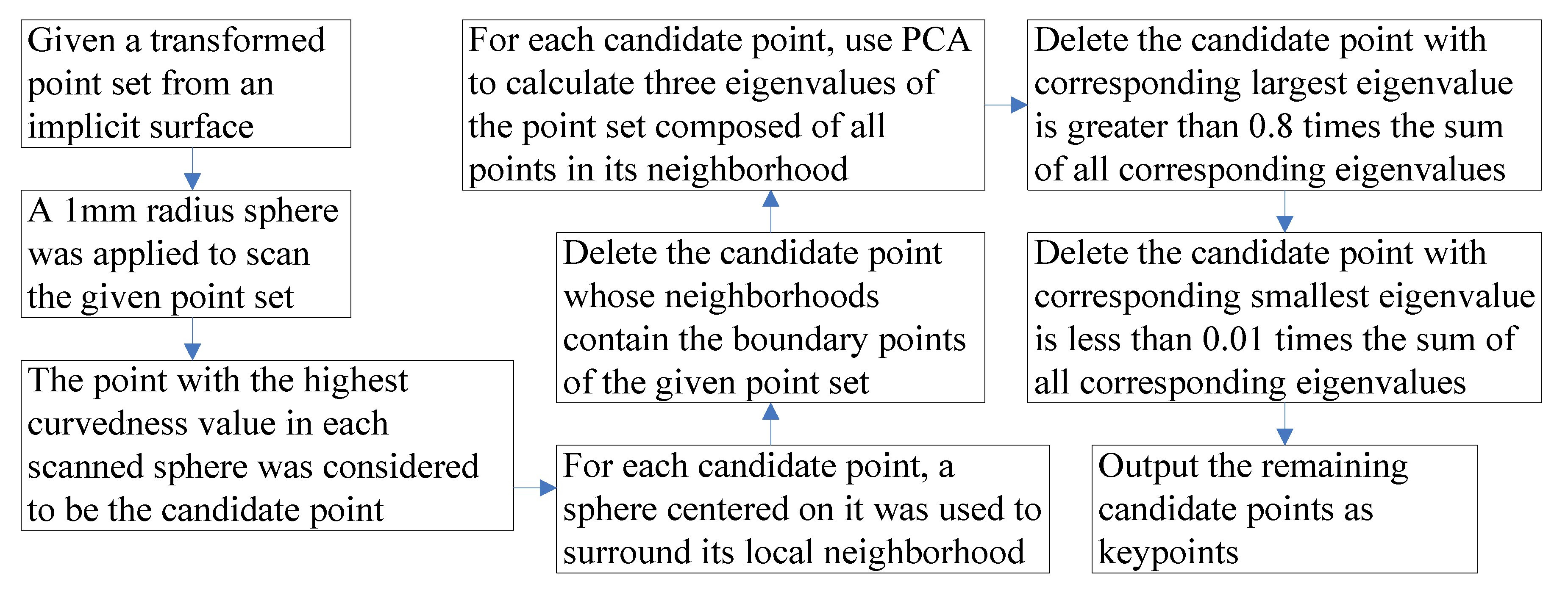
4.3. Proposed Keypoint Selection Method

In this step, we aim to select a set of potential keypoints insensitive to data variations, allowing the generation of the local and LJS feature set and accurate matching. Zhou et al. [8] presented a subtle keypoint selection method based on a square window. First, a 1 × 1 mm window was applied to scan the detected ear region in the range image, and the point corresponding to the highest curvedness value in each window was considered to be the candidate point. Second, for each candidate point, a sphere centered on it was used to surround its local neighborhoods. Third, they delete the candidate point whose local neighborhoods contain the boundary points. Fourth, the eigenvalues of the surrounded local neighborhoods associated with each candidate point were calculated by applying principal component analysis (PCA) [24]. Notably, some of the candidate points are deleted when the partial eigenvalues associated with them do not have a predefined interval. The final remaining candidate points are designated as keypoints. However, the pose robustness of the keypoint selection method based on a square window remains insufficient. Thus, we present a keypoint selection method based on a sphere with better pose robustness than that based on a square window. We follow the same keypoint selection procedure described above [8], substituting a 1 × 1 mm² window with 1-mm radius sphere and range image with a transformed point set. Figure 4 show the flow chart for selecting keypoint.

4.4. Definition of the Local Feature

The local SPHIS feature representation of 3D data can be directly utilized for the local data cropped using the sphere feature representation [8]. Let $kp$ be a keypoint and $S$ be a surface patch cut by a sphere with a radius of 14 mm centered at $kp$. $S_1$, $S_2$, $S_3$, and $S_4$ represent four surface patches with distances between any point constituting the surface patch and a $kp$ of less than 3.5, 3.5–7, 7–10.5, and 10.5–14 mm, respectively.

For the patch $S_k$, let $p_j^{\left(k\right)}$ represent the point that it contains, and $C_v\left(p_j^{\left(k\right)}\right)$ and $S_I\left(p_j^{\left(k\right)}\right)$ be the curvedness and shape index of point $p_j^{\left(k\right)}$, respectively, where $j=1,\dots ,n_k$. Here, $n_k$ represents the total number of points in $S_k$. Equations (4) and (5) were used to calculate $S_I\left(p_j^{\left(k\right)}\right)$ and $C_v\left(p_j^{\left(k\right)}\right)$, respectively, by substituting $p$ with $p_j^{\left(k\right)}$. The set $\left\{x_i^{\left(k\right)}|1\le i\le 16,i\in N\right\}$ contains the centers of the bins, and the weight $h\left(x_i^{\left(k\right)}\right)$ of the $i^{th}$ bin can be calculated as:

$$h\left(x_i^{\left(k\right)}\right)={\displaystyle {\sum }_{j=1}^{n_k}Co\left(p_j^{\left(k\right)},x_i^{\left(k\right)},i\right)}$$

(6)

where $Co\left(p_j^{\left(k\right)},x_i^{\left(k\right)},i\right)=\{\begin{array}{cc}{C}_v\left(p_j^{\left(k\right)}\right)·\left(1-\frac{\left|S_I\left(p_j^{\left(k\right)}\right)-x_i^{\left(k\right)}\right|}{0.0625}\right)& \left|S_I\left(p_j^{\left(k\right)}\right)-x_i^{\left(k\right)}\right|\le 0.0625\\ 0& otherwise\end{array}$.

The HIS descriptor of $S_k$ is $\left(h\left(x_1^{\left(k\right)}\right),\dots ,h\left(x_{16}^{\left(k\right)}\right)\right)/{\displaystyle {\sum }_{i=1}^{16}h\left(x_i^{\left(k\right)}\right)}$, whereas the SPHIS descriptor of the surface patch $S$ is established by concatenating the HIS descriptors of $S_1$, $S_2$, $S_3$, $S_4$, $S_I\left(kp\right)$, and $C_v\left(kp\right)$. Figure 5 show the flow chart for calculating the local descriptor.

4.5. Proposed LJS Feature

As mentioned in previously conducted studies [4], the objective of the TNG method is to obtain a set of keypoint correspondences that can maintain rigid constraints. However, when the TNG method is complete, a set of strategy pairs may exist in which each strategy pair satisfies the following conditions. As shown in Figure 6b,c, the two local surface patches associated with every strategy have similar shapes; however, variation is observed with respect to the relative pose of two local surface patches associated with a strategy pair from a particular sample and the relative pose of another two local surface patches associated with a strategy pair obtained from another sample (Figure 6a). The combined structure of two surface patches from a particular sample cannot rigidly match the joint structure of two surface patches obtained from another sample (Figure 6d), resulting in several inaccurate matching strategies obtained using the 3D images from two subjects. Thus, the TNG method makes it difficult to identify the ear using the relative pose information of two local surface patches, which may narrow the interclass difference.

Herein, we propose a PSPHIS descriptor to encode information that is sensitive to the relative pose of two surface patches. Figure 7 denotes the process for establishing the PSPHIS descriptor. First, we construct a two-keypoint structure containing two keypoints and two surface patches cropped using two sphere cuts, which are centered on both the keypoints with radius $r_{dks}$. $r_{dks}$ is set to 7 mm such that the surface patch associated with the two-keypoint structure is almost equivalent in size to a surface patch associated with the SPHIS descriptor. Second, for each cropped surface patch, the points contained within it are divided into two subsets using an additional plane cut to obtain shape information related to the relative pose of the two surface patches contained in the two-keypoint structure. Every plane contains its associated keypoint and is perpendicular to the connection line between two keypoints constituting the two-keypoint structure. Thus, two subsurface patches associated with each keypoint are formed, as shown in Figure 7f–j. For each subsurface patch, we constructed an HIS descriptor in accordance with the procedure described in Section 4.4. Finally, for the two-keypoint structure, four HIS descriptors of four subsurface patches associated with the two-keypoint structure as well as the shape index and the curvedness of two keypoints associated with the two-keypoint structure were concatenated to form a 68-dimensional PSPHIS descriptor. In addition, we used the PSPHIS descriptor to represent the LJS feature of a two-keypoint structure. Figure 8 show the flow chart for calculating the LJS descriptor.

The PSPHIS descriptor is invariant to the rigid body transformation of the ear similar to the SPHIS descriptor [8]. Every surface patch cropped using the hemisphere cut associated with a two-keypoint structure does not change with ear transformation, because the relative displacement between any surface point and two keypoints will not be changed by the rigid body transformation of the ear. The PSPHIS descriptor can effectively identify ears using the information that is sensitive to the relative pose of the two surface patches.

4.6. Proposed Local and LJS Matching Engine

We propose a local and LJS matching engine to obtain the similarity score. The proposed matching engine is based on the recently discovered game theoretic object recognition technique [17] and comprises two stages. The complete process of the first stage comprises candidate strategy set generation, payoff matrix construction, optimal solution search, detection of the strategy representing non-outlier correspondence, and probe and gallery–ear–model registration. In the second stage, we follow the same process described above, adding 3D point filtering before payoff matrix construction, modifying the process of candidate strategy set generation, and deleting the process of the probe and gallery–ear–model registration.

We describe the proposed matching engine in detail. In the first stage, we first generate a candidate strategy set. All the keypoints and their local SPHIS descriptors were acquired from the probe and gallery ear models. For each local SPHIS descriptor in the probe ear model, all the local SPHIS descriptors contained in the gallery ear model with an $L_2$-norm distance of less than 0.1 were defined as its similar local features [12], and not more than its five similar local features with relatively smaller $L_2$-norm distances were retained [4]. As a result, for each local SPHIS descriptor $SPHIS\left(a_i\right)$ in the probe ear model, the keypoint $a_i$ associated with it and keypoint $b_{i,j}$ associated with it retained each of its similar local SPHIS features in the gallery ear model constituted a candidate strategy $\left(a_i,b_{i,j}\right)$. This procedure was repeated for every local SPHIS descriptor in the probe ear model, resulting in a set of candidate strategies.

$$CS=\left\{\left(a_i,b_{i,j}\right)|\left(a_i,b_{i,j}\right)\in K{S}_P\times K{S}_G,b_{i,j}\in d{n}_5\left(a_i\right)and{\Vert SPHIS\left(a_i\right)-SPHIS\left(b_{i,j}\right)\Vert }_2<0.1\right\}$$

(7)

Here, for the SPHIS local descriptor $SPHIS\left(a_i\right)$ in the probe ear model, $d{n}_5\left(a_i\right)$ represents a set of keypoints associated with it that retained its similar SPHIS local features in the gallery ear model, and $K{S}_P$ and $K{S}_G$ represent the set of all the keypoints that make up the probe and gallery ear model, respectively. Second, a payoff matrix is constructed to enforce their respective Euclidean constraints [4] and their respective LJS feature constraints. The values of each element in the payoff matrix associated with a probe ear model $P$ and a gallery ear model $G$ are calculated using the following equation:

$$e\left(\left(a_{i^{\prime }},b_{i^{\prime },j^{\prime }}\right),\left(a_{i^{″}},b_{i^{″},j^{″}}\right)\right)=\frac{\min \left({\Vert a_{i^{\prime }}-a_{i^{″}}\Vert }_2,{\Vert b_{i^{\prime },j^{\prime }}-b_{i^{″},j^{″}}\Vert }_2\right)}{\max \left({\Vert a_{i^{\prime }}-a_{i^{″}}\Vert }_2,{\Vert b_{i^{\prime },j^{\prime }}-b_{i^{″},j^{″}}\Vert }_2\right)}.$$

(8)

This function considers pairs of strategies $\left(a_{i^{\prime }},b_{i^{\prime },j^{\prime }}\right),\left(a_{i^{″}},b_{i^{″},j^{″}}\right)\in P\times G$ and allots an earning $e$ based on the given $l_2$-norm distances of the candidate strategy pair. Furthermore, we impose a constraint on two strategies that share a keypoint to modify the payoff of the game as follows [7].

$$e\left(\left(a_{i^{\prime }},b_{i^{\prime },j^{\prime }}\right),\left(a_{i^{″}},b_{i^{″},j^{″}}\right)\right)=0,if{a}_{i^{\prime }}=a_{i^{″}}or{b}_{i^{\prime },j^{\prime }}=b_{i^{″},j^{″}}$$

(9)

When the difference between the distances of two keypoints from $P$ and that of the remaining two keypoints from $G$ is greater than 1.5 mm, the two strategies containing these four keypoints cannot coexist after completing the proposed matching engine [4,12]. Therefore, the payoff for the game can be fine-tuned as follows.

$$e\left(\left(a_{i^{\prime }},b_{i^{\prime },j^{\prime }}\right),\left(a_{i^{″}},b_{i^{″},j^{″}}\right)\right)=0,if{\Vert a_{i^{\prime }}-a_{i^{″}}\Vert }_2-{\Vert b_{i^{\prime },j^{\prime }}-b_{i^{″},j^{″}}\Vert }_2>1.5\mathrm{mm}$$

(10)

As described in Section 4.5, it is difficult to align the two structures when the relative pose of the two surface patches contained in a two-keypoint structure and the relative pose of the two surface patches contained in another two-keypoint structure vary. Thus, the strategy pair associated with both the two-keypoint structures cannot coexist within the preserved subset strategies with the proposed matching engine result. Since the proposed PSPHIS descriptor can effectively represent the relative pose of the two surface patches, we propose a simple payoff matrix optimization method. After all the two-keypoint structures and their respective PSPHIS descriptors were acquired from the probe and gallery ear models, for a strategy pair, we calculated the payoff value as follows:

$$e\left(\left(a_{i^{\prime }},b_{i^{\prime },j^{\prime }}\right),\left(a_{i^{″}},b_{i^{″},j^{″}}\right)\right)=0,if\Vert PSPHIS\left(S_{a_{i^{\prime }}{a}_{i^{″}}}\right)-PSPHIS\left(S_{b_{i^{\prime },j^{\prime }}{b}_{i^{″},j^{″}}}\right)\Vert >thp$$

(11)

where $S_{a_{i^{\prime }}{a}_{i^{″}}}$ and $S_{b_{i^{\prime },j^{\prime }}{b}_{i^{″},j^{″}}}$ are the two-keypoint structures; $a_{i^{\prime }}$ and $a_{i^{″}}$ are the keypoints of $S_{a_{i^{\prime }}{a}_{i^{″}}}$; and $b_{i^{\prime },j^{\prime }}$ and $b_{i^{″},j^{″}}$ are the keypoints of $S_{b_{i^{\prime },j^{\prime }}{b}_{i^{″},j^{″}}}$. To determine the optimal threshold $thp$, the $thp$ values (i.e., 0.05, 0.1, 0.15, and 0.2) were verified, where $thp=0.1$ achieved the best performance.

Third, to rapidly achieve Nash equilibrium, we used the infection–immunization dynamics introduced by Rota Bulò and Bomze [25], exhibiting a computation complexity of $O\left(N\right)$ for each iteration, where $N$ is the size of a candidate set of strategies $CS$.

Fourth, after reaching a stable state, the occupied share of all the strategies is concatenated to vector $X$. Further, we use a subset of strategies $C{S}^{\left(1\right)}$ to represent the final solution, where each contained strategy occupied more than $0.5\max \left(X\right)$ share.

Finally, we register ear models $P$ and $G$ by aligning the keypoint correspondences [8] that constitute the set $C{S}^{\left(1\right)}$.

In the second stage, we first perform 3D point filtering. Based on the registered probe–gallery ear models pair, we delete the outliers from the probe ear model (when the $l_2$-norm distance from a probe point to its corresponding gallery point is greater than 10 mm, the probe point is considered an outlier [4], points corresponding to outliers and points that do not correspond to the probe ear model points from the gallery ear model). Second, we propose a modified method to build a candidate strategy set. The candidate strategy set used in the second stage depends on the registered ear models obtained in the first stage [4], and it is difficult to match the local features of keypoints near occlusion in the first stage of the proposed matching engine owing to the influence of occlusion. Therefore, we select each strategy contained in set $C{S}^{\left(1\right)}$ as a candidate strategy and the corresponding keypoints (surrounded by the corresponding voxels) that are near the deleted point and have similar local features to form the candidate strategy.

$$CS=C{S}^{\left(1\right)}\cup C{S}^{\prime }$$

(12)

where

$$\begin{array}{l}C{S}^{\prime }=\{\left(a_i,b_{i,j}\right)|a_{i}correspondto{b}_{i,j},b_{i,j}\in d{n}_5\left(a_i\right),{\Vert SPHIS\left(a_i\right)-SPHIS\left(b_{i,j}\right)\Vert }_2<0.1,\\ a_i\in A{S}_P,b_{i,j}\in A{S}_G,atleast\exists dp,{\Vert a_i-dp\Vert }_2\le 14mm\}\end{array}$$

Here, $dp$ represents each deleted point. $A{S}_P$ and $A{S}_G$ represent the set of all the retained keypoints that make up the probe and gallery ear model, respectively. Later, we will perform the remaining process of the first stage for the retained registered ear models by deleting the process of the probe and gallery–ear–model registration. To obtain point correspondences from a pair of registered ear models, we use the voxel correspondences extraction method [4]. First, PCA [24] is used to calculate the normal direction, i.e., the direction of the third principal component of all 3D points that constitute a gallery ear model. Then, a surface voxelization method [8] is used to voxelize the registered pair of ear models surrounded by a 3D bounding box, the bottom plane of which is perpendicular to the normal direction. Finally, we use a “normal projection” matching strategy [4], which is robust to outliers, to obtain the corresponding voxels in the registered ear models, where the connecting line of the center points of a pair of voxels contained in each voxel correspondence is parallel to the normal direction. We designate the probe ear model point and gallery–ear–model point surrounded by the corresponding voxels as corresponding points. Algorithm 1 and Figure 9 describe the local and LJS matching engine. Figure 10 shows an example of how the keypoint correspondences are obtained from a pair of ear models.

Algorithm 1: Local and LJS matching engine

1. Given keypoint sets $K{S}_G$ and $K{S}_P$, the local SPHIS feature descriptor of keypoint $d$, the two-keypoint structure $S_{d_1{d}_2}$ associated with a pair of keypoints $\left(d_1,d_2\right)$, the LJS PSPHIS feature descriptor of the two-keypoint structure $S_{d_1{d}_2}$, where $d\in K{S}_P\cup K{S}_G$, $d_1,d_2\in K{S}_D$, and $K{S}_D\in D$. Here, $D\in \left\{P,G\right\}$. • First stage  2. Use (7) to establish a candidate strategy set $CS$.  3. Use (8–11) to construct the payoff matrix.  4. Search the optimal solution, obtain the share of every strategy in set $CS$, and concatenate the share of all the strategies to vector $\overline{X}$.  5. Extract set $C{S}^{\left(1\right)}$ composed by every strategy with a share greater than $0.5\overline{X}$ in set $CS$  6. Register models $P$ and $G$. • Second stage  7. 3D point filtering. Obtain keypoint sets $A{S}_G$ and $A{S}_P$ from the keypoints of the gallery and probe ear model, respectively, the local SPHIS feature descriptor of retained keypoint $d$ from the models generated by the retained point set, the two-keypoint structure $S_{d_1{d}_2}$ associated with a pair of keypoints $\left(d_1,d_2\right)$, the LJS PSPHIS feature descriptor of the two-keypoint structure $S_{d_1{d}_2}$, where $d\in A{S}_P\cup A{S}_G$, $d_1,d_2\in A{S}_D$, $A{S}_D\in D$. Here, $D\in \left\{P,G\right\}$  8. Use (12) to establish a candidate strategy set $CS$  9. Perform Steps 3–5.  10. Output $\left|C{S}^{\left(1\right)}\right|$ as similarity match score.

Similar to our previous TNG [4], the purpose of our proposed matching engine is to obtain the similarity match score between a probe–gallery pair under the GT pipeline. However, the difference between our proposed matching engine and TNG are as follows. (1) The input probe ear model is different. The input probe ear model in TNG is generated by pixels surrounded by a proposal in the range image, while the input probe ear model in our proposed matching engine is generated by 3D points obtained by a more accurate ear segmentation method based on PointNet++ [7]. (2) In TNG [4], the payoff matrix is generated according to geometrical constraints, while in our proposed matching engine, the generating process of the payoff matrix is constrained by the geometric and LJS features. (3) TNG can only delete the outliers that are far away from the ear surface in the probe ear model and the surface points of the gallery ear model corresponding to these outliers, while the proposed matching engine can delete the points that meet the above requirements and also delete the gallery–ear–model surface points that fail to correspond to the surface points of the probe ear model based on the ear segmentation result. Therefore, in comparison with TNG, our proposed matching engine can recognize ears more robustly by integrating robust ear segmentation results as well as local and LJS features.

5. Brief Review of the Holistic Matching Engine

This section reviews a SOA holistic matching [8] method that is with our local and LJS feature-matching engine. Since the registered voxelized probe and gallery ear models have been obtained by performing the local and LJS matching engine, we directly vectorize the voxelized probe–gallery ear models pair [8] and then use the cosine similarity measure [8] to calculate the global matching score of this pair of ear models.

6. Fusion

We use a transform-based feature fusion technique to exploit the local and LJS, and we use holistic matching scores for effectively recognizing the ear [8]. First, the two aforementioned matching scores are used to generate two independent similarity matrices $S_i$, where $i=1$ denotes the similarity matrices associated with the local and LJS matching engine, $i=2$ denotes the similarity matrices associated with the holistic matching engine, and the size of $S_i$ is $s\left(P\right)\times s\left(G\right)$. Here, $s\left(P\right)$ and $s\left(G\right)$ represent the number of probe and gallery 3D ear models, respectively. Further, we transform each matching score contained in similarity matrices using a double sigmoid normalization scheme [26]. Finally, for each pair of ear model comprising a probe ear model and a gallery ear model, we use a weighted sum algorithm to calculate the final fusion score.

7. Experiments

We evaluated our method using the UND-J2 database and the pose variation subdatabase of UND-G to validate its feasibility and effectiveness. The UND-J2 database contains 1800 profile samples of 415 subjects. At least two samples were used per subject, where each sample is represented as a 3D point cloud. The pose of different samples of each subject is significantly similar. Figure 11 shows several ear regions extracted from this database. The pose variation subdatabase of UND-G contains 96 samples of 24 subjects from the UND database, where the pose of the four samples of each subject are straight-on, 15° off-center, 30° off-center, and 45° off-center. Experiments were conducted in the following five types of scenarios:

• Evaluation of segmentation result;
• Ear recognition with random occlusion, where occlusions are close to the probe ear surface;
• Ear recognition with random occlusion, where all points contained in the random occlusion-presented random distribution in region from the ear surface to the camera lens;
• Ear recognition with pose variation; and
• Comparison with another ear recognition method.

7.1. Evaluation of Segmentation Result

To verify the effect of the ear segmentation method, we first train PointNet++ with a dataset of 16881 shapes from 16 classes [7]. Later, from the UND-J2 database, we randomly select 415 samples of 415 subjects for fine-tuning PointNet++. In practice, the position of the occluding objects is unpredictable. Therefore, we first set up a randomly located cuboid whose bottom and top planes are on the respective bottom and top planes of a bounding box enclosing every probe 3D ear model; then, we simulate different intrusive occluding objects by substituting the surface point surrounded by the cuboid with a random point set between the ear and camera lens. The occlusion percentage is equal to the ratio of the number of surface voxels surrounded by the cuboid to the number of surface voxels surrounded by the bounding box of the probe ear, where the surface voxels were obtained from the voxelized probe 3D ear (Section 4.6). The distance between each point from the occlusion and the probe 3D ear is a random number belonging to the interval [0 mm, 10 mm]. This ensures that the shape of the occluding object is considerably different from that of the ear surface, making the separation of the occluding object from the ear difficult. We label the 3D shape according to the setting adopted by Yi et al. [27]. The voxel containing ground-truth 3D ear points partially occupied by automatically segmented 3D points are considered to be correctly segmented voxels.

Table 1. Segmentation accuracy (%).

Technique	Occlusion Percentage (%)
	0	10	20	30	40	50
PointNet++	93.0	91.3	89.1	86.8	84.2	81.4

summarizes the average segmentation accuracy based on per-voxel criterion [7]. The segmentation accuracy decreases with the increase of occlusion. An example ear segmentation result is visualized in Figure 12.

7.2. Ear Recognition with Random Occlusion Close to the Ear Surface

In the real world, the captured ear samples are probably partially occluded by the hair, earrings, earphones, or other objects near the ear. We performed experiments on the UND-J2 database by considering intrusive objects as the occlusion to evaluate our method with random object occlusions close to the ear. The gallery samples used in this study are the same as those of the training sample used in the ear segmentation experiment. We select one sample of each subject from the remaining UND-J2 database as the probe sample. We generate the 3D ear data affected by nearby occlusion in accordance with the procedure in Section 7.1. Figure 13 shows one ear sample with six random occlusion percentages at intervals of 10% between 0% and 50%. The experimental results are provided in the form of a rank-1 recognition rate at occlusion rates of 0%, 10%, 20%, 30%, 40%, and 50%. These results are presented in

Table 2. Comparison of the recognition performance (%) for various random occlusion rates (%). DFF: dual feature fusion 3D ear biometrics, ICP–LSV: iterative closest point with local surface variation, LHFFO: local and holistic feature fusion occlusion ear recognition, VICP: variant of the ICP method.

Technique	Occlusion Percentage (%)
	0	10	20	30	40	50
VICP	97.80	73.01	44.33	24.82	8.67	1.40
ICP–LSV	98.55	73.73	45.30	25.83	9.40	2.17
DFF	98.30	95.86	89.16	63.13	38.31	17.11
LHFFO	98.80	97.98	91.81	69.88	47.95	25.54
Proposed method	98.82	98.36	95.08	83.71	70.84	55.86

.

We compared this study with our previous local and holistic feature fusion occlusion ear recognition (LHFFO) method [4], iterative closest point with local surface variation (ICP–LSV) method [16], a variant of the ICP method (VICP) [9], and a dual feature fusion 3D ear biometrics (DFF) [8] in a scenario in which random occlusion close to the ear surface is generated by the same dataset. Table 2 presents the comparison results. The LHFFO method is ineffective because it is difficult to separate the ear surface from abnormal points when they are near the ear surface and only use two layer of features. Furthermore, the ICP–LSV [16] and VICP methods [10] tend to fail when the ear pits are occluded. Although the DFF method [12] does not depend on ear pit acquisition, it is sensitive to the initial keypoint matching results. However, the proposed method mainly constructs the payoff matrix using the local features around each keypoint, the LJS features of the surface around each pair of keypoints, and the holistic features of the fine segmented ear region. Therefore, this study can identify ears using low-, middle-, high-level features, and a fine segmented ear surface. This study can also more accurately mine the 3D shape information when compared with the state-of-the-art (SOA) 3D ear recognition methods using only OSPP. The proposed method outperformed the SOA 3D ear recognition method under all the occlusion percentages.

7.3. Ear Recognition with All Points in Random Occlusion-Presented Random Distribution in the Region from the Ear Surface to the Camera Lens

In practical applications, the occluding objects may be anywhere between the ear and the camera lens. To simulate this application scenario, we simulate different intrusive occluding objects for each probe sample. This simulation method is similar to the simulation method for different intrusive occluding objects described in Section 7.1. Here, the only difference is substituting a random positive number less than 10 mm with a random positive number less than the distance between the probe 3D ear and the camera lens.

Table 3. Rank-one recognition rate (%) under different percentages of random occlusion (%).

Technique	Occlusion Percentage (%)
	0	10	20	30	40	50
VICP	97.80	73.49	45.06	25.78	8.92	1.45
ICP–LSV	98.55	74.21	46.02	26.75	9.88	2.41
DFF	98.30	95.90	90.12	65.06	40.48	18.80
LHFFO	98.80	98.31	94.22	80.48	64.58	44.82
Proposed method	98.82	98.41	95.28	85.06	74.94	64.92

presents the rank-one recognition results of the proposed method and the existing LHFFO, DFF, ICP–LSV, and VICP biometrics. Our proposed method outperforms the four remaining 3D ear biometrics.

7.4. Ear Recognition with Pose Variation

Large pose variation of the ear, especially in case of out-of-plane rotation, may introduce self-occlusion and result in partial data problem. Nevertheless, the majority of the keypoints can be extracted in a stable manner, and the occlusion rate of the majority of the local surface patches remains limited and computable in case of self-occlusion. Therefore, the proposed PTLFF method can select a set of corresponding keypoints that maintains distance invariant in two samples of a subject and leads to two-sample alignment. We tested the pose robustness of the proposed method using the pose variation subset of UND-G.

All the 96 images obtained from 24 subjects were divided into four different poses. Then, the four poses were classified into the gallery, and probe sets and were cross-matched with each other. The recognition results are presented in

Table 4. Recognition performance (%) under different poses.

Probe/Gallery	Straight-On	15° Off	30° Off	45° Off
Straight-On		100	95.8	87.5
		[100,100, 100,100]	[95.8,87.5, 95.8,87.5]	[87.5,70.8, 87.5,70.8]
15° off	100		100%	91.7%
	[100,100, 100,100]		[100,100, 100,100]	[91.7,83.3, 91.7,87.5]
30° off	100%	100%		95.8%
	[100,91.7, 100,87.5]	[100,100, 100,100]		[95.8,87.5, 91.7,95.8]
45° off	87.5	91.7	100
	[83.3,58.3, 83.3,79.2]	[91.7,83.3, 91.7,87.5]	[100,83.3, 95.8,100]

. The results reported obtained by LHFFO [4], DFF [8], ICP–LSV [16], and VICP [10] are given in order from left to right and from top to bottom (in brackets), and the best results are presented in bold. As can be seen, the proposed method outperforms the existing methods for all galleries with different poses.

7.5. Comparison with Other Recognition Methods

We compare the proposed method with other SOA 3D ear biometric systems (

Table 5. Performance comparison.

Method	Number of SPG *	Ear Normalization	Rank-1 Recognition Rate (%)	Runtime (per Pair Sample)
VICP	1	Yes	97.8	5–8 s
ICP–LSV	1	Yes	98.55	2.72 s
DFF	1	No	98.3	0.02 s
LHFFO	1	No	98.8	0.019 s
Ganapathi and Prakash [9]	1	Yes	98.69	0.36 s
Proposed method	1	No	98.82	0.033 s

* SPG, samples per person in the gallery.

). The aforementioned experiments were performed using a 3-GHz PC with 4 GB RAM with the UND-J2 database. The VICP method [9] requires multiple iterations for registration and matching of the dense ear models, resulting in considerable time consumption. In contrast, the existing methods [4,8] and this study only use a sparse set of features to register samples and require a small number of vertices to register the ear models. However, the proposed method requires partial time to extract the PSPHIS LJS descriptor and local and LJS matching engine; therefore, it is slower than our previous LHFFO method [4].

We compare the pose robustness of these methods shown in Table 5. ICP-based methods [10,16] need to input the probe and gallery ear model, which have been roughly aligned. Ganapathi and Prakash [9] proposed an ear recognition method that fuses the features of two different modalities and reported good accuracy. Nevertheless, when extracting global features, their method needs to divide the input rectangular depth map of ear into 20 grids with fixed scale, extract features from each grid, and finally connect the features in a specified order, making it easy to extract features with great differences from 3D ear models with the same subject in different poses. Thus, VICP [10], ICP–LSV [16], and Ganapathi and Prakash’s method [9] in Table 5 require ear data normalization after ear data are cropped in order to be rotated into a unified pose. Nevertheless, our proposed method, the LHFFO [4] method, and the DFF [8] method use raw ear data. Furthermore, our method shows better robustness against rotation.

7.6. Training of the Data Fusion Parameters

Six parameters, i.e., ${\alpha }_1^l,{\alpha }_2^l,{\tau }^l,{\alpha }_1^h,{\alpha }_2^h$, and ${\tau }^h$, are trained for data fusion, where ${\alpha }_1^l,{\alpha }_2^l,{\tau }^l$ are associated with the local and LJS feature modality and ${\alpha }_1^h,{\alpha }_2^h,{\tau }^h$ are associated with the holistic feature modality. From the UND database, we use 73 probe samples of 73 distinct subjects to build the training set, where each subject was not contained in previous experiments. For constructing the validation set, we randomly select one sample of each subject from the remaining samples of all the trained subjects. We use the one-versus-all strategy to transform the multi-classification problem to several two-classification problems [28]. We repeat the above steps, adding occlusion to the validation set as described in Section 7.2 and Section 7.3, respectively. Finally, we perform constrained optimization using the GlobalSearch framework provided by MATLAB to maximize the average area under receiver operating characteristic (ROC) curve of transformed two-classification problems [28].

8. Summary and Future Direction

Herein, we proposed a novel PTLFF method to address large occlusions close to the ear surface during OSPP ear recognition. The ear recognition experiments with various occlusion levels at random locations close to the ear surface were performed on UND datasets to demonstrate the effectiveness of the proposed method. When applied to the ear samples affected by a random large nearby occlusion, the proposed method achieved suitable SOA identification performance. However, the time involved in our proposed method is relatively longer when compared with that involved in our previous method [4] because of the high computational overhead. For the UND-J2 database, the average runtime per pair sample is 0.033 s, which is considerably higher than that reported in our previous study (0.019 s/pair samples) [4] primarily because the partial runtime is utilized for PSPHIS descriptor extraction and local and LJS matching engine. Therefore, our future study will focus on reducing the recognition time.

References

1. Emeršič, Z.; Meden, B.; Peer, P.; Struc, V. Evaluation and analysis of ear recognition models: Performance, complexity and resource requirements. In Neural Computing and Applications; Springer: Berlin, Germany, 2018; pp. 1–16. [Google Scholar]
2. Iannarelli, A.V. Ear Identification (Forensic Identification Series); Paramont: Fremont, CA, USA, 1989. [Google Scholar]
3. Pflug, A.; Busch, C. Ear biometrics: A survey of detection, feature extraction and recognition methods. IET Biomet. 2012, 1, 114–129. [Google Scholar] [CrossRef] [Green Version]
4. Zhu, Q.; Mu, Z. Local and holistic feature fusion for occlusion-robust 3D ear recognition. Symmetry 2018, 10, 565. [Google Scholar] [CrossRef] [Green Version]
5. Tian, L.; Mu, Z. Ear recognition based on deep convolutional network. In Proceedings of the International Congress on Image and Signal Processing, BioMedical Engineering and Informatics (CISP-BMEI), Datong, China, 15–17 October 2016; pp. 437–441. [Google Scholar]
6. Alshazly, H.; Linse, C.; Barth, E.; Martinetz, T. Ensemble of deep learning models and transfer learning for ear recognition. Sensors 2019, 19, 4139. [Google Scholar] [CrossRef] [PubMed] [Green Version]
7. Qi, C.R.; Yi, L.; Su, H.; Guibas, L.J. Pointnet++: Deep hierarchical feature learning on point sets in a metric space. In Advances in Neural Information Processing Systems; AbeBooks: Victoria, BC, Canada, 2017; pp. 5099–5108. [Google Scholar]
8. Zhou, J.; Cadavid, S.; Abdel-Mottaleb, M. An efficient 3-D ear recognition system employing local and holistic features. IEEE Trans. Inf. Forensics Secur. 2012, 7, 978–991. [Google Scholar] [CrossRef]
9. Ganapathi, I.I.; Prakash, S. 3D ear recognition using global and local features. IET Biom. 2018, 7, 232–241. [Google Scholar] [CrossRef]
10. Yan, P.; Bowyer, K.W. Biometric recognition using 3D ear shape. IEEE Trans. Pattern Anal. Mach. Intell. 2007, 29, 1297–1308. [Google Scholar] [CrossRef] [PubMed]
11. Chen, H.; Bhanu, B. Human ear recognition in 3D. IEEE Trans. Pattern Anal. Mach. Intell. 2007, 29, 718–737. [Google Scholar] [CrossRef] [PubMed]
12. Cadavid, S.; Abdel-Mottaleb, M. 3-D ear modeling and recognition from video sequences using shape from shading. IEEE Trans. Inform. Forensics Secur. 2008, 3, 709–718. [Google Scholar] [CrossRef] [Green Version]
13. Sun, X.; Zhao, W. Parallel registration of 3D ear point clouds. In Proceedings of the 8th International Conference on Information Technology in Medicine and Education (ITME), Fuzhou, China, 23–25 December 2016; pp. 650–653. [Google Scholar]
14. Prakash, S. False mapped feature removal in spin images based 3D ear recognition. In Proceedings of the 3rd International Conference on Signal Processing and Integrated Networks (SPIN), Noida, India, 11–12 February 2016; pp. 620–623. [Google Scholar]
15. Tharewal, S.; Gite, H.; Kale, K.V. 3D face & 3D ear recognition: Process and techniques. In Proceedings of the International Conference on Current Trends in Computer, Electrical, Electronics and Communication (CTCEEC), Mysore, India, 8–9 September 2017; pp. 1044–1049. [Google Scholar]
16. Zhang, Y.; Mu, Z.; Yuan, L.; Zeng, H.; Chen, L. 3D ear normalization and recognition based on local surface variation. Appl. Sci. 2017, 7, 104. [Google Scholar] [CrossRef] [Green Version]
17. Albarelli, A.; Rodola, E.; Bergamasco, F.; Torsello, A. A non-cooperative game for 3D object recognition in cluttered scenes. In Proceedings of the International Conference on 3D Imaging, Modeling, Processing, Visualization and Transmission, Hangzhou, China, 16–19 May 2011; pp. 252–259. [Google Scholar]
18. Albarelli, A.; Rodola, E.; Torsello, A. Fast and accurate surface alignment through an isometry-enforcing game. Pattern Recognit. 2015, 48, 2209–2226. [Google Scholar] [CrossRef]
19. Goldman, R. Curvature formulas for implicit curves and surfaces. Comp. Aided Geom. Des. 2005, 22, 632–658. [Google Scholar] [CrossRef]
20. Zhang, J.; Hon, J.; Wu, T.; Zhong, L.; Gong, S.; Tang, Y. Rapid surface reconstruction algorithm for 3D scattered point cloud model. J. Comput. Aided Des. Comput. Graph. 2018, 30, 235–243. [Google Scholar] [CrossRef]
21. Wendland, H. Piecewise polynomial, positive definite and compactly supported radial functions of minimal degree. Adv. Comput. Math. 1995, 4, 389–396. [Google Scholar] [CrossRef]
22. Xu, H.; Fang, X.; Hu, L. Computing point orthogonal projection onto implicit surfaces. J. Comput. Aided Des. Comput. Graph. 2008, 20, 1641–1646. [Google Scholar]
23. Dorai, C.; Jain, A.K. COSMOS-A representation scheme for 3D free-form objects. IEEE Trans. Pattern Anal. Mach. Intell. 1997, 19, 1115–1130. [Google Scholar] [CrossRef] [Green Version]
24. Jolliffe, I. Principal component analysis. In International Encyclopedia of Statistical Science; Springer: Berlin/Heidelberg, Germany, 2011; pp. 1094–1096. [Google Scholar]
25. Bulò, S.R.; Bomze, I.M. Infection and immunization: A new class of evolutionary game dynamics. Games Econ. Behav. 2011, 71, 193–211. [Google Scholar] [CrossRef] [Green Version]
26. Cappelli, R.; Maio, D.; Maltoni, D. Combining fingerprint classifiers. In Proceedings of the International Workshop on Multiple Classifier Systems, Cagliari, Italy, 21–23 June 2000; pp. 351–361. [Google Scholar]
27. Yi, L.; Kim, V.G.; Ceylan, D.; Shen, I.-C.; Yan, M.; Su, H.; Lu, C.; Huang, Q.; Sheffer, A.; Guibas, L. A scalable active framework for region annotation in 3d shape collections. ACM Trans Graph. 2016, 35, 210. [Google Scholar] [CrossRef]
28. Zhang, X.; Jiang, C. Improved SVM for learning multi-class domains with ROC evaluation. In Proceedings of the International Conference on Machine Learning and Cybernetics, Hong Kong, China, 19–22 August 2007; pp. 2891–2896. [Google Scholar]
Figure 1. Images of the partially occluded ears. Ear is partially occluded by (a) finger; (b) hair; (c) earrings and (d) earphone.
Symmetry 12 00078 g001
Figure 2. System diagram of the proposed method.
Symmetry 12 00078 g002
Figure 3. Flow chart for calculating the shape index and curvedness of a surface point of an implicit surface.
Symmetry 12 00078 g003
Figure 4. Flow chart for selecting keypoint.
Symmetry 12 00078 g004
Figure 5. Flow chart for calculating the local descriptor.
Symmetry 12 00078 g005
Figure 6. Pair of mismatched strategies. (a) A diagram of a pair of mismatched strategies and two matched surface patches associated with (b) a strategy, (c) another strategy, and (d) a pair of strategies.
Symmetry 12 00078 g006
Figure 7. Pairwise surface patch cropped using a hemisphere cut-structured histogram with an indexed shape (PSPHIS) feature extraction. (a) 3D ear; (b) 3D ear with two spheres centered at two keypoints; (c) shape index map of the 3D ear; (d) curvedness map of the 3D ear; (e) the surface patches are surrounded by spheres with the two keypoints marked; (f) four subsurface patches dividing the cropped surface patches with different color points for each subsurface patch; (gj) four subsurface patches shown with two keypoints connected by a dotted line; (k) two keypoints connected by a dotted line; (lo) HIS descriptor with 16 bins calculated using the corresponding subsurface patches; (p) shape index and curvedness of the corresponding two keypoints; and (q) final PSPHIS feature descriptor.
Symmetry 12 00078 g007
Figure 8. Flow chart for calculating the local joint structural (LJS) descriptor.
Symmetry 12 00078 g008
Figure 9. Flow chart for local and LJS matching engine.
Symmetry 12 00078 g009
Figure 10. Example of obtaining keypoint correspondences for a pair of ears from same person. (a) Detected keypoints. (b) Detected non-outlier keypoint correspondences by a local and LJS matching engine.
Symmetry 12 00078 g010
Figure 11. Several extracted ear regions.
Symmetry 12 00078 g011
Figure 12. Sample ear segmentation result.
Symmetry 12 00078 g012
Figure 13. Different percentages of occlusions in the probe sample surrounded by the ear bounding box.
Symmetry 12 00078 g013