A Novel Isomap-SVR Soft Sensor Model and Its Application in Rotary Kiln Calcination Zone Temperature Prediction

Abstract

Soft sensing technology has been proved to be an effective tool for the online estimation of unmeasured or variables that are difficult to directly measure. The performance of a soft sensor depends heavily on its convergence speed and generalization ability to a great extent. Based on this idea, we propose a new soft sensor model, Isomap-SVR. First, the sample data set is divided into training set and testing set by using self-organizing map (SOM) neural network to ensure the fairness and symmetry of data segmentation. Isometric feature mapping (Isomap) method is used for dimensionality reduction of the model input data, which could not only reduce the structure complexity of the proposed model but speed up learning speed, and then the Support Vector Machine Regression (SVR) is applied to the regression model. A novel bat algorithm based on Cauchy mutation and Lévy flight strategy is used to optimize parameters of Isomap and SVR to improve the accuracy of the proposed model. Finally, the model is applied to the prediction of the temperature of rotary kiln calcination zone, which is difficult to measure directly. The simulation results show that the proposed soft sensor modeling method has higher learning speed and better generalization ability. Compared with other algorithms, this algorithm has obvious advantages and is an effective modeling method.

1. Introduction

In petrochemical, chemical, iron, and steel metallurgy and other process industries, due to economic or technical constraints, there are often some process variables that cannot be measured online or are difficult to measure using real sensors. However, these variables are usually key process parameters or quality indicators. These variables are usually determined by off-line sample analysis in the laboratory, so it is difficult to use them in the feedback signal of online control system. Online monitoring of these variables is an important guarantee to ensure safety, smooth production, efficient operation, and greater economic benefits. The main problem of quality control in the process industry is how to realize the estimation of these unpredictable variables online. Soft sensors are usually used to solve these problems. Soft sensor technology uses the idea of indirect measurement, multiple regression analysis, support vector machine, neural network, and other technical means to estimate the dominant variable through a certain correlation between the auxiliary variable and the dominant variable. It has the advantages of less investment, simple maintenance, and fast response.

Rotary kiln is the main production equipment of iron ore pellet, and the temperature of calcination zone is one of the key technical indexes to determine the quality of finished pellet. Increasing the temperature control level of calcination zone is of great significance to improving the quality of finished pellet. However, when the rotary kiln is running, Thermocouple signal transmission slip-ring is prone to poor contact and the temperature measurement signal is unstable. In addition, the thermocouple has an extremely short service life under the strong oxidation and high temperature environment. Therefore, to replace the faulty thermocouple, the rotary kiln must stop running, which seriously affects the production. Other non-contact temperature measurement methods (such as infrared temperature measurement, etc.) have extremely low accuracy under the harsh environment. Therefore, it is of great significance to establish a soft sensor model to predict the temperature of rotary kiln calcining zone. Due to the complex mechanism of pellet roasting, strong coupling, and nonlinear characteristics, conventional mechanism modeling and regression analysis methods are difficult to establish an accurate temperature measurement model. Intelligent modeling methods such as neural network, support vector machine and rough set are effective methods to solve the problem of soft measurement of key process variables in complex nonlinear systems. For soft sensor of calcining zone temperature of rotary kiln, literature [1] established a soft sensor model of calcining zone temperature of rotary kiln by using an improved limit learning machine. Literature [2] adopted a soft sensor model of calcining zone temperature of rotary kiln based on multi-model fusion technology based on least square support vector machine, and optimized the model structure with PSO algorithm. Literature [3] used t-s fuzzy neural network and model transfer method to establish a soft sensor model of calcining zone temperature of rotary kiln. Support Vector machine (SVR) is an effective tool for nonlinear modeling of complex systems. Currently, SVR algorithm has been widely used in the research field of soft sensing. Literature [4] used Gaussian SVR and cat mapping prediction, cloud model, and hybrid particle swarm optimization algorithm to establish the urban traffic flow prediction model, achieving better prediction effect than the SVR prediction method alone. Literature [5] established a soft sensor model of ethylene polymerization process by using PCA method. First, PCA method was used to reduce the dimension of sample data, and then particle swarm optimization algorithm was used to optimize the parameters of the SVR model. Literature [6] studies a time-dependent regression algorithm for online support vector machines (SVM), which overcomes the time-varying characteristics of the object. Simulation and industrial applications show that it has good accuracy. Literature [7] studied an evolutionary fuzzy SVR soft sensor model and successfully applied it to the prediction of welding residual stress. Soft sensor modeling is essentially a data-driven modeling method. Data preprocessing and model parameter selection will affect the model accuracy. The SVR algorithm has been improved and the prediction accuracy has been improved in the above literature; however, the data preprocessing and the model optimization process have not been combined, so the model accuracy still has some room for improvement. This paper proposes an Isomap-SVR soft sensing model based on improved bat algorithm optimization and applies the soft sensor model to the prediction of rotary kiln calcination zone temperature. The model uses Isomap method to reduce the dimension of the sample data. The parameter K of the Isomap and the structure of SVR model are joint optimized using an improved bat algorithm. The simulation results verify the effectiveness of the proposed method.

2. Pellet Production Process and Soft Sensor Model

2.1. Pellet Production Process

Pellet production equipment is generally composed of grate, rotary kiln [8] and ring cooler. The pellets with diameters of 9~16 mm obtained in the pelleting process were preheated in the grate and then entered the rotary kiln from the kiln tail. The ball will move towards the kiln head with the rotation of the rotary kiln. The calcination flame is injected from the kiln head to the kiln tail, and the raw ball is solidified by the roasting of the high temperature flame and the action of the heat radiation in the kiln [9]. After calcination, the pellets enter the ring cooler from the kiln head for cooling, and the hot smoke generated by the ring cooler returns to the grate as a heat source for preheating the raw pellets. In normal operation of rotary kiln, the temperature of calcination belt should be controlled at 1250 °C, to ensure the quality of pellets and avoid the damage of the kiln body. The temperature of rotary kiln calcination zone is difficult to be measured stably. Currently, the fuel quantity and other operating parameters of the system are generally adjusted by manual fire observation. As a result, the product quality is greatly affected by human factors, and the mass of finished pellet [10] fluctuates greatly.

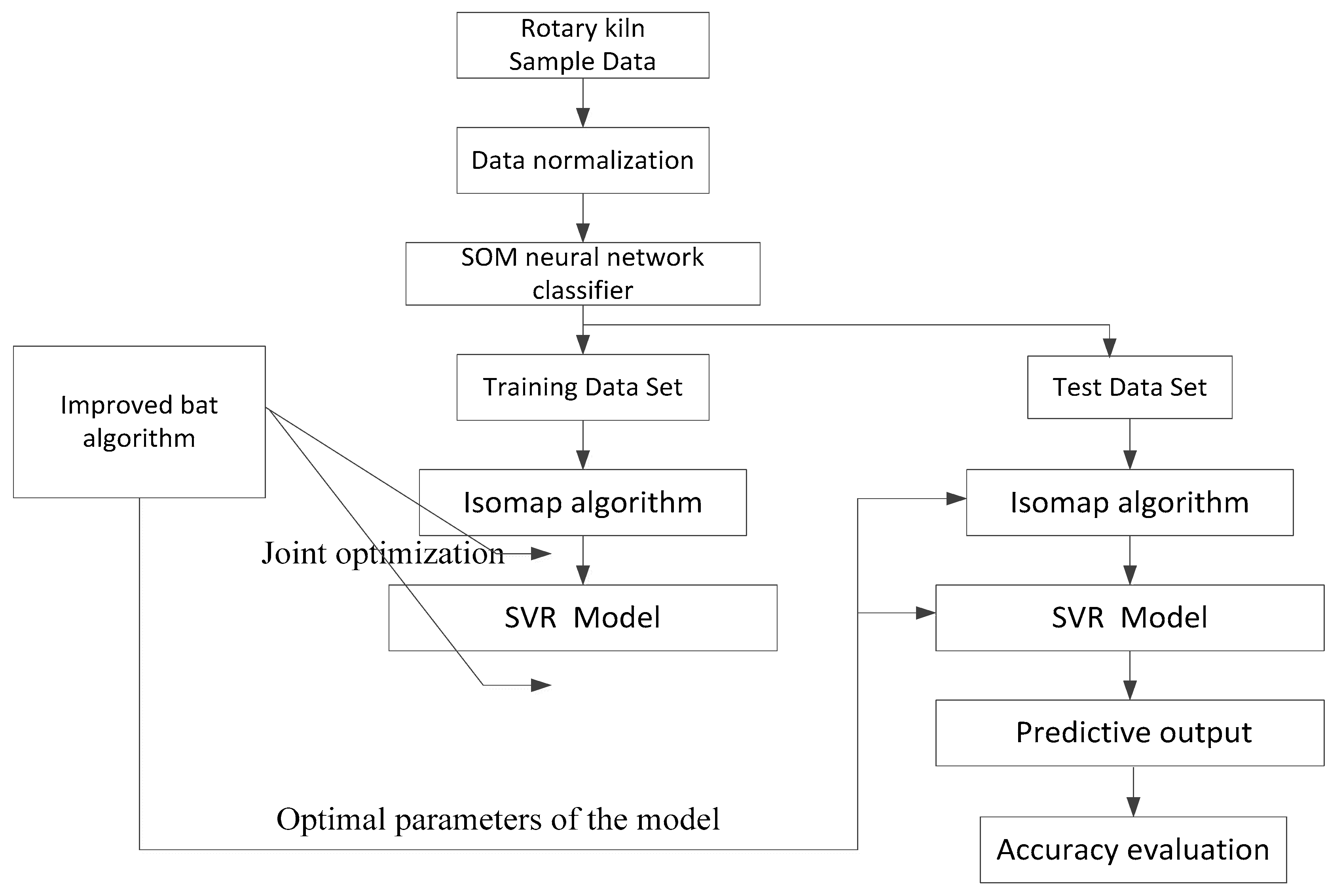
2.2. Soft Sensor Model Structure

The soft sensor method is an effective solution to the problem of temperature prediction of rotary kiln calcination zone [11]. In this paper, based on the mechanism of rotary kiln process characteristics and heat balance [12], we select 13 process variable related to the rotary kiln calcination zone temperature which are easily detected as the soft sensor input. They are coal injection amount, chain grate machine material thickness, the chain grate machine preheating section of the hood I temperature, chain grate machine preheating section II hood temperature, kiln head temperature and temperature of preheater, ring I period of air temperature, cold machine ring cooler II period of air temperature, drum cover specific temperature, convulsions hood temperature, cold chain grate machine speed, rotating speed of rotary kiln and ring pattern in speed. The output of the soft sensor model is the temperature of calcination zone, and the temperature signal obtained when the slip-ring thermocouple temperature transmitter works steadily. The lower the data dimension, the simpler the model structure, in order to simplify the model structure and realize the joint optimization of parameters K of the Isomap algorithm and the structure SVR model, we have designed the model structure as shown in Figure 1.

3. Data Dimension Reduction Processing Based on Isomap

Compared with traditional linear dimension reduction methods such as PCA [13] and MDS [14], Isomap is a globally optimized nonlinear dimension reduction algorithm. It replaces the Euclidean distance by geodesic distance, and extracts hidden nonlinear manifolds from high-dimensional data while retaining the inherent geometric characteristics of data. It is easier to achieve nonlinear reduction of high-dimensional data [15,16]. The implementation steps of Isomap [16] algorithm are as follows:

Step 1: For input sample $X={\left\{x_i\right\}}_{i=1}^S$, $x_i\in R^p$, p and S are dimension and rows of sample X, respectively. Set the neighborhood parameter K, Constructing $k$-Neighborhood Graph $G$. Calculate the Euclidean distance between each sample point and the remaining sample points $D_{ij}^E\left(i\ne j\right)$, if $x_j$ is one of the closet to k points of $x_i$, $E_{ij}$ is an edge of $G$ and the length is $D_{ij}^E$, finally the neighborhood weighting graph $G$ is obtained.

Step 2: Calculating Geodetic Distance Matrix D^M. The geodesic distance on a manifold is approximated by the shortest distance between the points, Obtain the geodetic distance matrix D^M = D^G, the shortest distance $D_{ij}^G$ can be obtained by Floyd iterative algorithm [17,18].

Step 3: Construct $q$ dimension embedding. Use MDS Method to Find Transform Matrix ${\tau }^G$.

$${\tau }^G=\frac{-HSH}{2}=\frac{-H((D_{ij}^M{)}^2)H}{2}$$

(1)

where:

$$H=(h_{ij})=\{\begin{array}{c}1-1/S,i=j\\ -1/S,i\ne j\end{array}$$

(2)

The eigenvalues of ${\tau }^G$ are sorted in descending order. If the matrix of the eigenvectors corresponding to the previous $q$ eigenvalues is $U$, the $q$ dimension embedding result of the output is as follows:

$$T_H=diag({\lambda }_1^{1/2},{\lambda }_2^{1/2},\dots ,{\lambda }_q^{1/2})U^T$$

(3)

In the Isomap algorithm, the neighborhood parameter K determines the result of dimensionality reduction, and then affects the accuracy of the soft sensor model. The value of K must be selected reasonably.

4. SVR Soft Sensor Modeling Optimized by Improved Bat Algorithm

4.1. SVR Algorithm

The core idea of Support Vector Machine Regression (SVR) [19] for nonlinear prediction is to find the optimal hyperplane so that the distance between sample data and the plane is the shortest. For the nonlinear sample set ${\{x_i,y_i\}}_{i=1}^N$ (y_i is the output of x_i, $N$ is the number of samples). SVR solves the nonlinear relationship between $x_i$ and $y_i$ by mapping input vector $x_i$ into high-dimensional feature space through nonlinear mapping $\varphi (\cdot )$ and linear regression [20]. Its high-dimensional linear regression function is:

$$f(x)={\omega }^T\varphi (x)+b$$

(4)

$\omega$ is a high-dimensional weight vector, $b$ is offset. If the penalty coefficient C is introduced, the relaxation factors ${\xi }_i$ and ${\xi }_i^{*}$, and the insensitive parameters $\epsilon$, $\omega$ and $b$ can be obtained by minimizing the objective function:

$$minJ=\frac{1}{2}{\Vert \omega \Vert }^2+C{\displaystyle \sum }_{i=1}^N({\xi }_i+{\xi }_i^{*})$$

(5)

$$s.t.\{\begin{array}{c}{y}_i-{\omega }^T\cdot \varphi \left(x\right)-b\le \epsilon +{\xi }_i^{*}\\ {\omega }^T\cdot \varphi \left(x\right)+b-y_i\le \epsilon +{\xi }_i\\ {\xi }_i^{*}\ge 0,{\xi }_i\ge 0\end{array}$$

(6)

The Lagrange multiplier is introduced to solve the quadratic programming problem with inequality constraints, Available:

$$f\left(x\right)={\displaystyle \sum }_{i=1}^N\left({\alpha }_i^{*}-{\alpha }_i\right)K\left(x_i,x_j\right)+b$$

(7)

In the formula: ${\alpha }_i$ and ${\alpha }_i$ are Lagrangian coefficients obtained by Lagrange multiplier [21] method, $K\left(x_i,x_j\right)$ is a nonlinear kernel function, In this paper, the Gauss function [22] is chosen as the kernel function:

$$K\left(x_i,x_j\right)=exp(-\frac{{\Vert x_i-x_j\Vert }^2}{2{\delta }^2})$$

(8)

The main parameters affecting the accuracy of SVR model are penalty coefficient C and kernel function width $\delta$.

4.2. Bat Algorithm and Its Improvement

4.2.1. Bat Algorithm

Bat Algorithm (BA) is a new intelligent optimization algorithm proposed by Yang in 2010 to simulate the bat echolocation behavior. It has been successfully applied in many function optimization problems [23]. For the optimization problem that the solution variable is $X={(x_1,x_2,\cdots ,x_d)}^T$ and the objective function is $f$(X). The implementation steps of the BA algorithm are as follows:

Step 1: Initial population number M, maximum pulse loudness A⁰, maximum pulse frequency R⁰, position moving range and initial velocity V⁰ of each bat, search pulse frequency range [f_min, f_max], loudness attenuation factor $\alpha$, frequency enhancement factor $\gamma$, maximum iteration number T and search precision $\epsilon$ of the algorithm. The initial position vector ${\left\{X_i^0\right\}}_{i=1}^M$ of each bat is randomly determined. Set the current iterations t = 1.

Step 2: Calculate the current optimal solution vector $X_{*}^t$ according to the fitness function. Update the search pulse frequency, speed, and position of each bat. The update formulas are as follows:

$$f_i=f_{\min }+(f_{\max }-f_{\min }){\beta }_i$$

(9)

$$V_i^t=V_i^{t-1}+[X_i^t-X_{*}^t]f_i$$

(10)

$$X_i^t=X_i^{t-1}+X_i^t$$

(11)

where $\beta$ is a $M$ dimensional random vector uniformly distributed on [0, 1], f_i is an acoustic frequency.

Step 3: Generate a random parameters R_rand between [0, 1]. For each bat, if R_rand > R_i, performs a local search, and $X_i^t$ performs a random perturbation to generate a new solution:

$$new{X}_i^t=X_{*}^t+\eta A^t$$

(12)

where: $\eta$ is a $M$-dimensional random vector uniformly distributed on [−1, 1], $A$^t is the average loudness of the current bat population.

Step 4: Generate a random parameters A_rand between [0, 1]. If A_rand < A_i, and $f(new{X}_i^t)<f(X_{*}^t)$, accept the new solution $new{X}_i^t$, then update $R_i^t$ and $A_i^t$ according to the following formula:

$$A_i^{t+1}=\alpha A_i^t$$

(13)

$$R_i^{t+1}=R_i^t[1-\exp (-\gamma t)]$$

(14)

where: $\alpha$ is the loudness attenuation coefficient, $\gamma$ is the frequency increase coefficient.

Step 5: If the minimum fitness meets the optimization requirement or the number of iterations is greater than $T$, the optimal fitness value and the optimal solution are output. Otherwise t = t + 1, and return to Step 2.

From the perspective of the algorithm itself, the basic BA achieves position update through speed update. There is no effective mechanism to escape from the local extremum. The algorithm is easy to premature and the search accuracy is poor [24,25,26].

4.2.2. Lévy Flight Strategy

To solve the shortcomings of the basic BA, this paper first introduces Lévy flight mechanism to improve the speed update formula of the basic BA. The 3D figure of Lévy flight process is shown in Figure 2.

From Figure 2, it can be observed that frequently small steps and occasional large step occur alternately during the process of Lévy flight, which will help the algorithm jump out of local minima.

Formula (15) is a new velocity update formula instead of Formula (10).

$$\{\begin{array}{c}{V}_i^t=V_i^{t-1}+\left[X_i^t-\left(1-c\right)X_{*}^t-c{X}_b^t\right]f_i\kappa \\ \kappa =\mu \cdot sign\left(rand-0.5\right)\oplus L{e}^{\prime }vy\end{array}$$

(15)

where $X_b^t$ is the current optimal value and $X_{*}^t$ is the global optimal value. $c$ and $\mu$ are random parameters between [0, 1], $sign()$ is a symbol function, symbol $\oplus$ is point multiplication, and random step length Lévy is from Lévy distribution:

$$L{e}^{\prime }vy~u=t^{\lambda }(1<\lambda \le 3)$$

(16)

Formula (15) takes the optimal value of the current generation as one of the parameters of speed update, which can effectively reduce the attraction intensity of bats to the global optimal value. At the same time, the Lévy flight mechanism can effectively avoid the premature of the algorithm.

4.2.3. Cauchy Mutation Strategy

Secondly, there is no mutation mechanism in BA. At the later stage of search, almost all individuals will gather around the optimal solution. If this solution is local optimal solution, the algorithm will fall into local minimum. In this paper, adaptive mutation mechanism is introduced to avoid premature.

The specific method is that if the fitness value does not change within K (K = 3) generation, it means that the algorithm falls into local optimum, and then produces a random number ${\omega }_{rand}$ between [0, 1], If ${\omega }_{rand}<p_t$ (Cauchy mutation probability), the individual bat carries out Cauchy mutation according to the formula (17).

$$X_i=X_i+X_i\times C\left(0,1\right)$$

(17)

The $C\left(0,1\right)$ in the formula is the standard Cauchy distribution. Since the Cauchy distribution is more prone to generate random numbers far from the origin than the Gaussian distribution, the range of mutation is larger, and it is easier to jump out of the local optimum.

The Cauchy mutation probability is:

$$P_t=0.3\sqrt{1-{(\frac{T-t}{T})}^2}$$

(18)

The probability of mutation increases as the increase of iterations t, which is more conducive to overcoming the local optimum.

Finally, to overcome the shortcomings of poor local search accuracy of BA, a variable step size local search strategy is proposed. Formula (12) is modified to:

$$new{X}_i^n+{(\frac{T-t}{T})}^2\eta A^t$$

(19)

where T is the max iterations of the algorithm, and $t$ is the current iterations. As the increase of iterations, the step length of local search will be smaller and smaller, and the precision of local search will be improved continuously. In this paper, the improved bat algorithm is named IBA.

The proposed IBA is evaluated on 6 typical test functions which listed in

Table 1. Benchmark functions.

Name	Function	D	Range	fopt
Shpere	$f_1(x)={\displaystyle {\sum }_{i=1}^D{x}_i^2}$	30	[−10,10]D	0
Schwefel 2.22	$f_2(x)={\displaystyle {\sum }_{i=1}^D\left|x_i\right|}+{\displaystyle {\prod }_{i=1}^D\left|x_i\right|}$	30	[−10,10]D	0
Ackley	$f_3(x)=-20\exp (-0.2\sqrt{1/D{\displaystyle {\sum }_{i=1}^D{x}_i^2}})-\exp (\frac{1}{D}{\displaystyle {\sum }_{i=1}^D\cos (2\pi x_i)})+20+e$	30	[−32,32]D	0
Griewank	$f_4(x)=1/4000{\displaystyle {\sum }_{i=1}^D{x}_i^2}-{\displaystyle {\prod }_{i=1}^D\cos (x_i/\sqrt{i})}+1$	30	[−600,600]D	0
Shifted Sum Square	$f_5(x)={\displaystyle {\sum }_{i=1}^{D}i{(x_i-\sqrt{i})}^2}$	30	[−100,100]D	0
Rotated Griewank	$f_6(x)=1/4000{\displaystyle {\sum }_{i=1}^D{y}_i^2}-{\displaystyle {\prod }_{i=1}^D\cos (y_i/\sqrt{i})}+1,$$where\begin{array}{c}\end{array}y=MxM\mathrm{is}\mathrm{an}\mathrm{orthogonal}\mathrm{matrix}$	30	[−600,600]D	0

. It compared with two classical optimization algorithm (i.e., BA and Particle swarm optimization algorithm (PSO) [27]), and two other recently improved BAs (i.e., EBA [28] and dBA [29]).

The functions are divided into three classes, f₁ and f₂ are unimodal functions, f₃ to f₄ are multimodal functions, f₅ and f₆ are rotated and shifted functions. The corresponding dimensions D, range, global minimum values f_opt of the functions are also listed in Table 1.

The parameters settings of the algorithms used in the comparisons are listed in

Table 2. Parameters settings of the algorithms used in the comparisons.

Algorithm	Reference	Parameters
BA	Ref. [23]	$\alpha =0.95$, $\gamma =0.95$, $f_{\min }=-2$, $f_{\max }=2$
PSO	Ref. [27]	$c_1=2$, $c_2=2$, ${\omega }_{\max }=1.0$, ${\omega }_{\min }=0.3$
EBA	Ref. [28]	${\xi }_{init}=0.6$, $n=3$
dBA	Ref. [29]	$r_0=0.1$, $r_{\infty }=0.7$, $A_0=0.9$, $A_{\infty }=0.6$
IBA	Present	$\alpha =0.95$, $\gamma =0.95$, $f_{\min }=-2$, $f_{\max }=2$

.

To make a fair comparison, all algorithms were tested using the same population size M = 30 and the same maximum number of iteration T = 500. For each trail, each algorithm was run 30 times independently on each test function. The convergence comparisons of all algorithms are graphically shown in Figure 3.

It can be seen from Figure 3 that the convergence speed and accuracy of the IBA algorithm are significantly better than that of BA, PSO, EBA, and dBA algorithm on f₁ to f₅. IBA has satisfactory performance on f₆, and only loses in dBA algorithm. It indicates that the overall performance of IBA is much better than other algorithms.

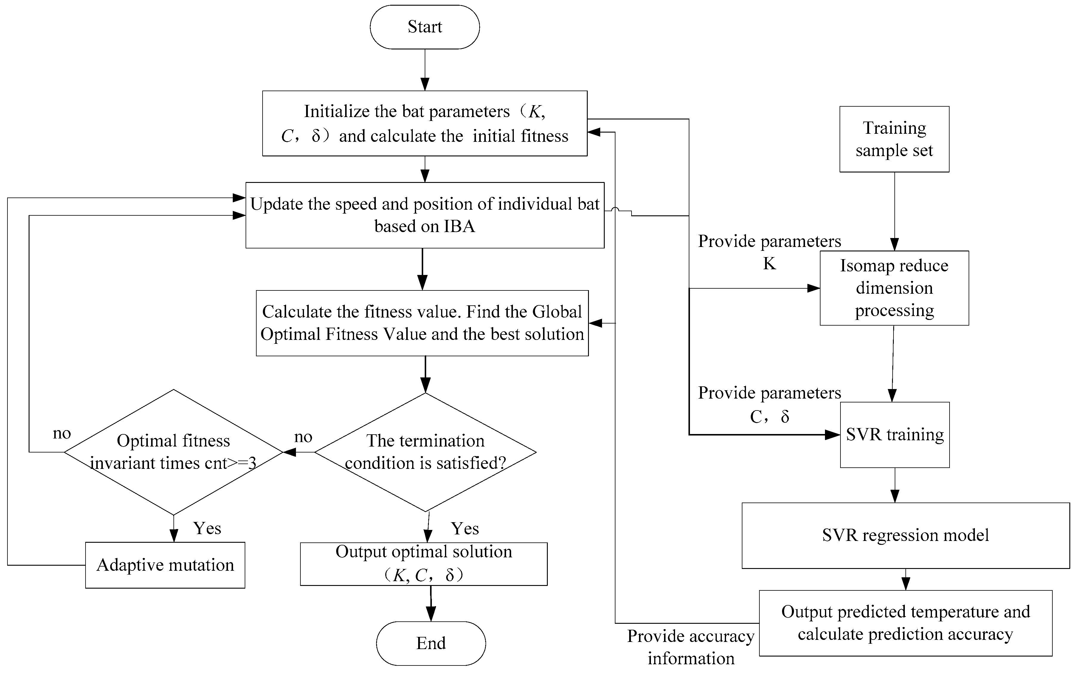
4.3. Soft Sensor Model Optimization Based on IBA Algorithm

As mentioned above, parameter K of the Isomap algorithm, penalty coefficient C and kernel function width $\delta$ of the SVR model determines the performance of the soft sensor model. In this paper, the parameters K, $C$ and $\delta$ are of the proposed soft sensor model are obtained by the IBA. The optimization process is as follows:

Step 1: Initialize the parameters of the BA, randomly generate the initial position $x_i^0=\{K_i^0,C_i^0,{\delta }_i^0\}$ of each bat, use the initial position of each bat as the parameter of the soft sensor model, apply the training data to train the SVR model, and calculate the fitness value. To ensure the robustness and fitting ability of the model and avoid overlearning, we select the determination coefficient R² and 5-fold cross verification accuracy Q²_cv5 as fitness function, namely:

$$fitness=\frac{1}{R^2{Q}^2{}_{cv5}}$$

(20)

where $R^2=1-\frac{{\displaystyle {\sum }_{i=1}^L{(y(i)-\stackrel{⌢}{y}(i))}^2}}{{\displaystyle {\sum }_{i=1}^L{(y(i)-\overline{y})}^2}}$, $Q_{cv5}^{{}^2}=1-\frac{{\displaystyle {\sum }_{i=1}^L{(y_{cv5}(i)-{\stackrel{⌢}{y}}_{cv5}(i))}^2}}{{\displaystyle {\sum }_{i=1}^L{(y_{cv5}(i)-\overline{y})}^2}}$L is the number of training samples.$y\left(i\right)$, ${\widehat{y}}_i$ and $\stackrel{-}{y}$ are the measured values, predicted values and average values of the measured values respectively.$y_{cv5}\left(i\right)$, ${\widehat{y}}_{cv5}\left(i\right)$ and $\stackrel{-}{y}$ are the mean values of the measured values of the cross validation set, the predicted value and the measured values of the training set respectively.

Step 2: Enter the BA iterative search process. An optimized search of the bat’s speed and position is based on the IBA.

Step 3: Termination condition judgment: If the number of iterations is greater than the specified maximum number of iterations or the fitness value meets the requirements, the algorithm ends and outputs the optimal bat position (the optimal parameters K, C and δ). Otherwise return to Step 2 to continue the search. Figure 4 shows the overall implementation flow chart of the algorithm.

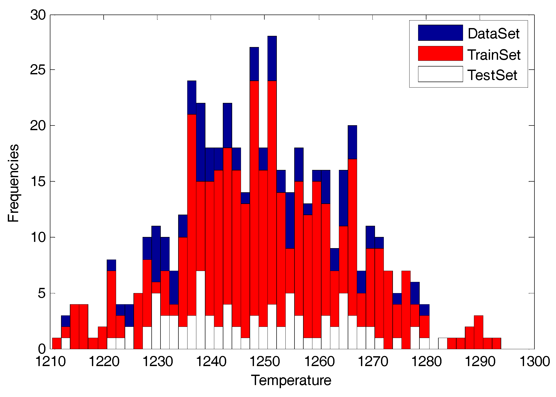
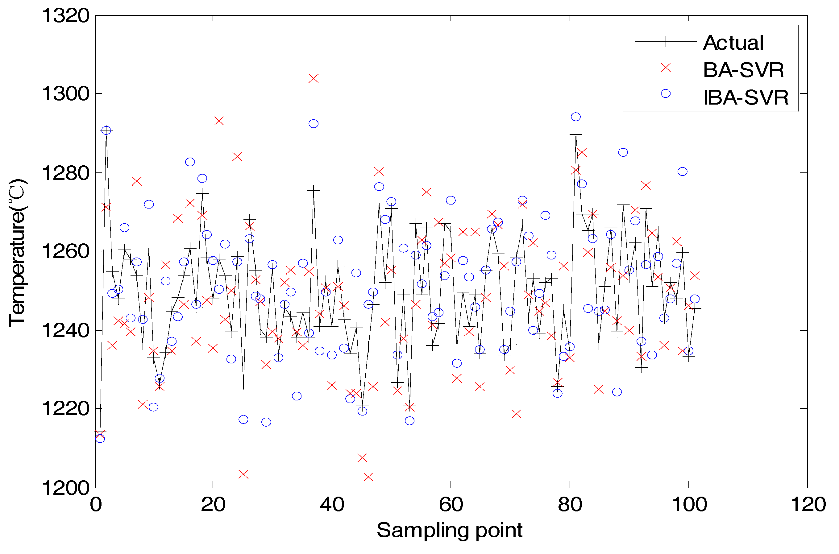
5. Simulation Analysis

To verify the effectiveness of the proposed method, we collected the production data of a 2 million ton/year pellet production line. First, we use 3δ criterion to eliminate [30] the anomaly data, and then standardize them [31]. Finally, we obtain 500 sets of modeling data.

(1) Simulation process and result in an experiment

a. Modeling dataset classification

To ensure the fairness of the model, the training data space is required to cover the testing data space as much as possible. Therefore, we use SOM neural network with clustering function [32] to divide the sample data set. First, a SOM neural network is established, the SOM neural network has 13 inputs and 16 hidden layer nodes. After 300 times of iterative training, the classification results of SOM network are shown in Figure 5.

Then, we randomly select 80% of the data in each hidden node of SOM neural network as model training data and the rest as model test data.

Figure 6 shows the distribution of training data, test data, and modeling data using SOM classification method in an experiment.

It can be seen from Figure 5 that the space of training data basically covers that of the test data.

b. Joint Optimization of Soft Sensor Models

Parameter K of the Isomap algorithm, penalty coefficient C and kernel function width $\delta$ of the SVR model determines the performance of the soft sensor model. When SVR model is trained, the allowable error of the model $\epsilon =1.25$ (that is, the values can satisfy R² and Q²_cv5 are both greater than 0.8). When using BA to optimize parameters of Isomap and SVR, the range of $K$ is [1, 100], the range of $C$ is [1, 100], and that of $\delta$ is [1, 100]. The initial parameters of the BA are: Bat population size M = 30, algorithm maximum search times N = 100, loudness attenuation coefficient $\alpha =0.95$, search frequency enhancement coefficient $\gamma =0.95$, search frequency range [−2, 2], bat speed range [−5, 5], bat individual position range [1, 100]. When optimizing the model, we select variables whose standard deviation of output variables of Isomap algorithm is greater than 0.05 as SVR model inputs.

After optimization, we get the following results: The best fitness value is 1.34, model fitting accuracy index R² = 0.887 and model robustness index Q²_cv5 = 0.841. (it is generally believed that R² > 0.7 and Q²_cv5 > 0.7 can establish a robust and reliable soft measurement model). K = 28, C = 76.235, δ = 2.014.

c. Result in this experiment

Figure 7 and Figure 8 respectively show the predicted value and prediction error curves of the calcination zone temperatures with the BA and IBA algorithm proposed in this paper.

It can be seen from Figure 7 and Figure 8 that the prediction accuracy of the proposed algorithm is significantly higher than that of the SVR model optimized by the basic Bat algorithm. The temperature prediction error of proposed algorithm is basically distributed in [−22.5 C, 22.5 C]. In production, the measuring range of thermocouple is 0~1500 °C, and the accuracy level is 1.5, so the maximum measurement error is 22.5. For this experiment, the prediction error of the proposed algorithm basically meets the actual measurement requirements.

(2) Statistical analysis

a. Compared with other algorithms

To verify the advantages of the proposed algorithm, we compared it with other algorithms (Each algorithm running 30 times independently, and SOM neural network is used to divide the sample data into training sample and test sample for each run), and the results are shown in

Table 3. Accuracy comparison of different modeling methods.

Dimensionality Reduction Method	Isomap				PCA
Modeling Method	GA-SVR	PSO-SVR	BA-SVR	IBA-SVR	IBA-SVR
$R{a}_{AD}<22.5{}^{°}\mathrm{C}$	95.3%	95.7%	96.3%	98.6%	96.9%
$R{a}_{AD}<37.5{}^{°}\mathrm{C}$	98.3%	98.8%	98.8%	99.7%	99.1%
Min_R2	0.794	0.822	0.816	0.841	0.842
Max_R2	0.911	0.921	0.891	0.922	0.921
Mean_R2	0.855	0.853	0.852	0.862	0.859
Min_Q2CV5	0.741	0.757	0.755	0.813	0.786
Max_Q2CV5	0.866	0.839	0.821	0.871	0.857
Mean_Q2CV5	0.821	0.823	0.829	0.851	0.836
Min_Q2ext	0.731	0.817	0.822	0.831	0.811
Max_Q2ext	0.832	0.855	0.869	0.874	0.862
Mean_Q2ext	0.811	0.831	0.847	0.851	0.836

.

In Table 3, $R{a}_{AD}<22.5{}^{°}\mathrm{C}$ and $R{a}_{AD}<37.5{}^{°}\mathrm{C}$ represent the proportion of test samples with absolute deviations less than 22.75 °C (Meet the demand of instrument with accuracy class of 1.5) and 37.5 °C (Meet the index of instrument with accuracy class of 2.5) in 30 tests; R² represents the fitting ability of the model. The larger is R², the stronger learning ability of the model to the training sample. Min_R², Max_R² and Mean_R², represent the maximum, minimum, and average values of R² of each algorithm in 30 experiments, respectively. Q²_CV5 represents the robustness of the model. The larger is Q²_CV5, the better robustness of the model. Q²_ext represents the prediction ability of the model for independent external test samples, and the value range is [0, 1]. The larger the is Q²_ext, the stronger external prediction ability of the model. The formula of Q²_ext is:

$$Q_{ext}^2=1-\frac{{\displaystyle {\sum }_{i=1}^V{(y(i)-\stackrel{⌢}{y}(i))}^2}}{{\displaystyle {\sum }_{i=1}^V{(y(i)-\overline{y})}^2}}$$

(21)

where $V$ is the number of test samples; $y\left(i\right)$ is the actual output of test samples, $\widehat{y}\left(i\right)$ is the model predictive output of test samples; $\overline{y}$ is the average output of training samples. Min_Q²_ext, Max_Q²_ext and Mean_Q²_ext, represent the maximum, minimum, and average values of Q²_ext of each algorithm in 30 experiments, respectively.

From the statistical results in Table 1, we can draw the following conclusions:

(1)

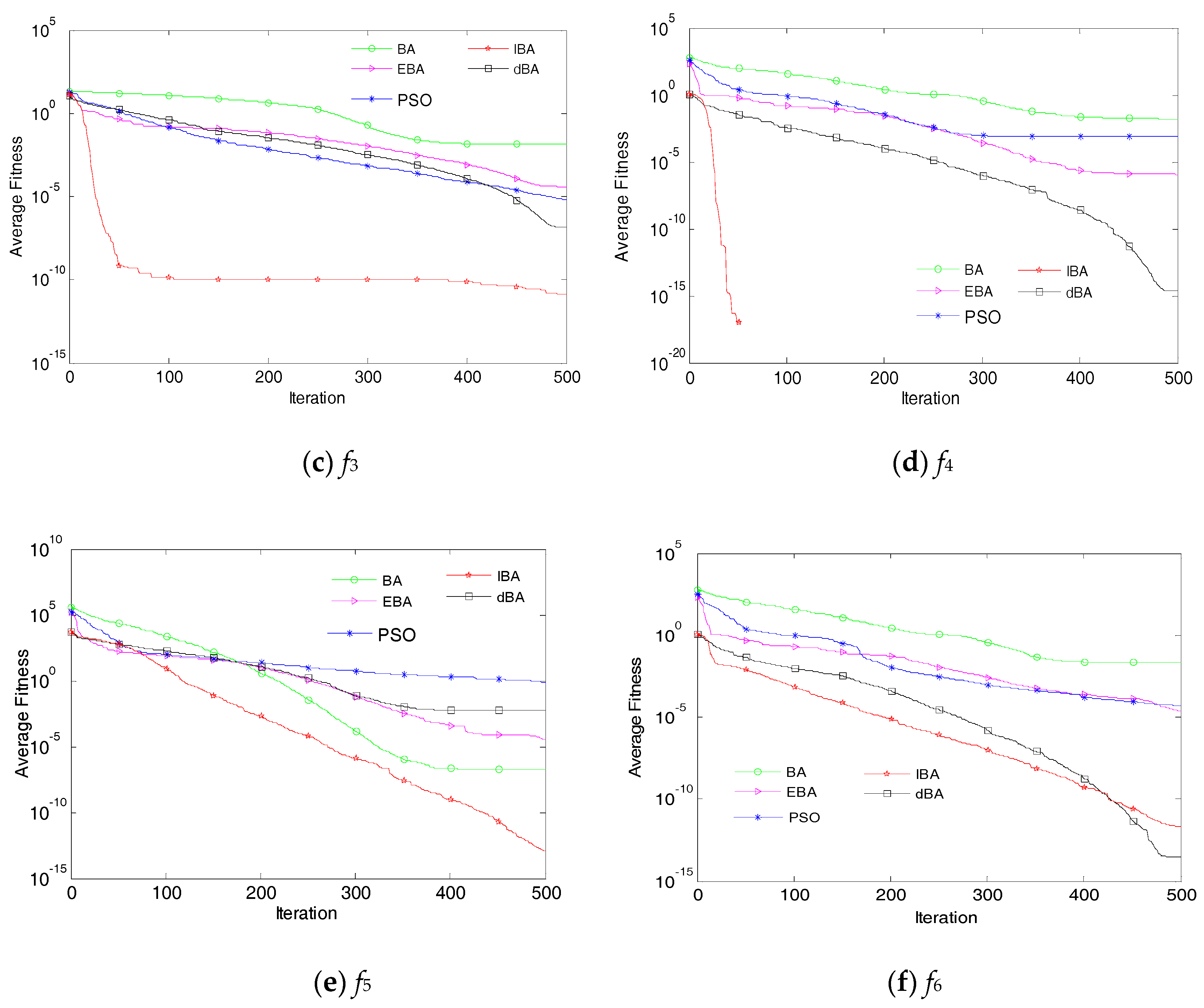
For Isomap data segmentation method, the value of R², Q²_CV5 and Q²_ext of the IBA-SVR algorithm proposed in this paper are better than those of the comparison algorithm. Therefore, the optimization performance of IBA algorithm for SVR model is better than that of other comparison algorithms.

(2)

By comparing the dimensionality reduction methods of Isomap and PCA data under IBA-SVR model, we can see that the model performance of dimensionality reduction using Isomap algorithm is better.

(3)

The joint to optimization of Isomap and SVR model using IBA algorithm effectively improves the prediction accuracy of the model. 98.6% of the prediction results meet the accuracy requirements of level 1.5 instruments, and 97.7% of the prediction results meet the accuracy requirements of level 2.5 instruments.

b. Comparison of Data Segmentation Methods

To prove the superiority of SOM neural network in segmenting sample data, we compared it with the method of randomly segmenting under the proposed Isomap-SVR model. We have carried out 30 experiments, and the experimental results are shown in

Table 4. Influence of Data Segmentation Methods on Model Performance.

Method of Data Segmentation		Random	SOM
Training Data	Min_R2	0.835	0.841
	Max_R2	0.912	0.922
	Mean_R2	0.859	0.862
	Min_Q2CV5	0.753	0.813
	Max_Q2CV5	0.891	0.871
	Mean_Q2CV5	0.821	0.851
Test Data	Min_Q2ext	0.741	0.831
	Max_Q2ext	0.896	0.874
	Mean_Q2ext	0.816	0.851

.

From the statistical results in Table 4, we can draw the following conclusions:

(1)

Considering the fitting ability, different data segmentation methods have little influence on the fitting ability of the model.

(2)

Considering the robustness of the model, the model established by the method of randomly segmented data fluctuates more than that established by the method of SOM neural network.

(3)

Considering the external prediction ability of the model, the external prediction ability of the model established by the method of SOM neural network segmentation data is more stable.

Therefore, the SOM neural network data segmentation method is more suitable to build a stable soft sensor model of rotary kiln temperature.

6. Conclusions

In this paper, a novel Isomap-SVR soft sensor modeling method is presented and the calcination zone temperature of the rotary kiln is chosen for simulation. The sample data of rotary kiln system are divided into training data and test data by SOM neural network, which ensures the fairness of modeling data. An IBA is studied, and its advantages are verified by a set of representative test functions. It is used to jointly optimize parameters of Isomap and SVR models to ensure the rationality of parameters of the soft sensor model. The simulation results show that the proposed algorithm has the advantages of good fitting ability, strong robustness, and generalization ability compared with the comparison algorithms. The algorithm has a good application prospect. Applying the algorithm to the prediction of the calcination zone temperature of the rotary kiln can obtain a higher accuracy, which has an important guiding significance for the safe production and optimal operation of the pellet production process.

References

1. Boateng, A.A.; Barr, P.V. A Thermal-Model for the Rotary Kiln Including Heat-Transfer within the Bed. Int. J. Heat Mass Transf. 1996, 39, 2131–2147. [Google Scholar] [CrossRef]
2. Tian, Z.; Li, S.; Wang, Y.; Wang, X. A multi-model fusion soft sensor modelling method and its application in rotary kiln calcination zone temperature prediction. Trans. Inst. Meas. Control. 2015, 38, 110–124. [Google Scholar]
3. Zhang, L.; Gao, X.W.; Wang, J.S.; Zhao, J. Soft-Sensing for Calcining Zone Temperature in Rotary Kiln Based on Model Migration. J. Northeast. Univ. 2011, 32, 175–178. [Google Scholar]
4. Li, M.W.; Hong, W.C.; Kang, H.G. Urban traffic flow forecasting using Gauss–SVR with cat mapping, cloud model and PSO hybrid algorithm. Neurocomputing 2013, 99, 230–240. [Google Scholar] [CrossRef]
5. Shi, X.; Chi, Q.; Fei, Z.; Liang, J. Soft-Sensing Research on Ethylene Polymerization Based on PCA-SVR Algorithm. Asian J. Chem. 2013, 25, 4957–4961. [Google Scholar] [CrossRef]
6. Kaneko, H.; Funatsu, K. Application of online support vector regression for soft sensors. AIChE J. 2014, 60, 600–612. [Google Scholar] [CrossRef]
7. Edwin, R.D.J.; Kumanan, S. Evolutionary fuzzy SVR modeling of weld residual stress. Appl. Soft Comput. 2016, 42, 423–430. [Google Scholar] [CrossRef]
8. Hou, Y.; Wei, S. Method for Mass Production of Phosphoric Acid with Rotary Kiln. U.S. Patent 10,005,669, 26 June 2018. [Google Scholar]
9. Phummiphan, I.; Horpibulsuk, S.; Rachan, R.; Arulrajah, A.; Shen, S.-L.; Chindaprasirt, P. High calcium fly ash geopolymer stabilized lateritic soil and granulated blast furnace slag blends as a pavement base material. J. Hazard. Mater. 2018, 341, 257–267. [Google Scholar] [CrossRef]
10. Konrád, K.; Viharos, Z.J.; Németh, G. Evaluation, ranking and positioning of measurement methods for pellet production. Measurement 2018, 124, 568–574. [Google Scholar] [CrossRef] [Green Version]
11. Tian, Z.; Li, S.; Wang, Y.; Wang, X. SVM predictive control for calcination zone temperature in lime rotary kiln with improved PSO algorithm. Trans. Inst. Meas. Control. 2017, 40, 3134–3146. [Google Scholar]
12. Yin, Q.; Du, W.-J.; Ji, X.-L.; Cheng, L. Optimization design and economic analyses of heat recovery exchangers on rotary kilns. Appl. Energy 2016, 180, 743–756. [Google Scholar] [CrossRef]
13. Kim, K.I.; Jung, K.; Kim, H.J. Face recognition using kernel principal component analysis. IEEE Signal Process. Lett. 2002, 9, 40–42. [Google Scholar]
14. Bengio, Y.; Paiement, J.; Vincent, P.; Delalleau, O.; Roux, N.; Ouimet, M. Out-of-sample extensions for lle, isomap, mds, eigenmaps, and spectral clustering. In Advances in Neural Information Processing Systems; 2004; pp. 177–184. Available online: https://dl.acm.org/doi/10.5555/2981345.2981368 (accessed on 12 December 2019).
15. Hannachi, A.; Turner, A.G. Isomap nonlinear dimensionality reduction and bimodality of Asian monsoon convection. Geophys. Res. Lett. 2013, 40, 1653–1658. [Google Scholar] [CrossRef] [Green Version]
16. Hannachi, A.; Turner, A. Monsoon convection dynamics and nonlinear dimensionality reduction vis Isomap. In Proceedings of the EGU General Assembly Conference, Vienna, Austria, 22–27 April 2012; EGU General Assembly Conference Abstracts. p. 8534. [Google Scholar]
17. Jing, L.; Shao, C. Selection of the Suitable Parameter Value for Isomap. J. Softw. 2011, 6, 1034–1041. [Google Scholar] [CrossRef]
18. Orsenigo, C.; Vercellis, C. Linear versus nonlinear dimensionality reduction for banks’ credit rating prediction. Knowl. Based Syst. 2013, 47, 14–22. [Google Scholar] [CrossRef]
19. Smola, A.J.; Schölkopf, B. A tutorial on support vector regression. Stat. Comput. 2004, 14, 199–222. [Google Scholar] [CrossRef] [Green Version]
20. Sammon, J.W. A nonlinear mapping for data structure analysis. IEEE Trans. Comput. 1969, 100, 401–409. [Google Scholar] [CrossRef]
21. Bertsekas, D.P. Constrained Optimization and Lagrange Multiplier Methods; Academic Press: Cambridge, MA, USA, 2014. [Google Scholar]
22. Golub, G.H.; Welsch, J.H. Calculation of Gauss Quadrature Rules. Math. Comput. 1969, 23, 221–230. [Google Scholar] [CrossRef]
23. Yang, X.S. A New Metaheuristic Bat-Inspired Algorithm. Comput. Knowl. Technol. 2010, 284, 65–74. [Google Scholar]
24. Subsequently. A Novel Hybrid Bat Algorithm with Harmony Search for Global Numerical Optimization. J. Appl. Math. 2013, 2013, 233–256. [Google Scholar]
25. Yang, X.S.; Deb, S. Cuckoo Search via Lévy Flights. In Proceedings of the World Congress on Nature & Biologically Inspired Computing (NaBIC), Coimbatore, India, 9–11 December 2009; IEEE: Piscataway, NJ, USA, 2010; pp. 210–214. [Google Scholar]
26. Wang, G.-G.; Gandomi, A.H.; Zhao, X.; Chu, H.C.E. Hybridizing harmony search algorithm with cuckoo search for global numerical optimization. Soft Comput. 2014, 20, 273–285. [Google Scholar] [CrossRef]
27. Wang, Y.K.; Chen, X.B. Improved multi-area search and asymptotic convergence PSO algorithm with independent local search mechanism. Kongzhi Yu Juece/Control Decis. 2018, 33, 1382–1390. [Google Scholar]
28. Ghanem, W.A.H.M.; Jantan, A. An enhanced Bat algorithm with mutation operator for numerical optimization problems. Neural Comput. Appl. 2019, 31, 617–651. [Google Scholar] [CrossRef]
29. Chakri, A.; Khelif, R.; Benouaret, M.; Yang, X.-S. New directional bat algorithm for continuous optimization problems. Expert Syst. Appl. 2017, 69, 159–175. [Google Scholar] [CrossRef] [Green Version]
30. Shen, X.; Fu, X.; Zhou, C. A combined algorithm for cleaning abnormal data of wind turbine power curve based on change point grouping algorithm and quartile algorithm. IEEE Trans. Sustain. Energy 2018, 10, 46–54. [Google Scholar] [CrossRef]
31. Gupta, S.; Perlman, R.M.; Lynch, T.W.; McMinn, B.D. Normalizing Pipelined Floating Point Processing Unit. U.S. Patent 5,058,048, 15 October 1991. [Google Scholar]
32. Pedrycz, W. Conditional fuzzy clustering in the design of radial basis function neural networks. IEEE Trans. Neural Netw. 1998, 9, 601–612. [Google Scholar] [CrossRef]
Figure 1. Soft sensor model structure.
Symmetry 12 00167 g001
Figure 2. 3D figure of Lévy flight.
Symmetry 12 00167 g002
Figure 3. The convergence comparisons of all algorithms. (a) Convergence Curve of sphere Function (f1) (b) Convergence Curve of Schwefel 2.22 Function (f2) (c) Convergence Curve of Ackley Function (f3) (d) Convergence Curve of Griewank Function (f4) (e) Convergence Curve of Shifted Sum Square Function (f5) (f) Convergence Curve of Rotated Griewank Function (f6).
Symmetry 12 00167 g003aSymmetry 12 00167 g003b
Figure 4. Algorithm flow chart.
Symmetry 12 00167 g004
Figure 5. SOM neural network classification results.
Symmetry 12 00167 g005
Figure 6. Distribution of sample data, training data, and test data in an experiment.
Symmetry 12 00167 g006
Figure 7. Model Prediction Output Contrast Diagram.
Symmetry 12 00167 g007
Figure 8. Prediction error comparison chart.
Symmetry 12 00167 g008