Research on Collaborative Planning and Symmetric Scheduling for Parallel Shipbuilding Projects in the Open Distributed Manufacturing Environment

Abstract

In the current distributed manufacturing environment, more extensive enterprise cooperation is an effective means for shipbuilding companies to increase the competitiveness. However, considering the project scale and the uneven production capacity between the collaborative enterprises, a key issue for shipbuilding companies is to effectively combine the product-oriented project tasks and the specialized production-oriented plants. Due to information privatization, the decision-making process of project planning and scheduling is distributed and symmetric. Existing project scheduling methods and collaboration mechanisms in the shipbuilding industry are somehow inefficient. The aim of the research is to provide an assistant decision-making method to support effective task dispatching and multi-party cooperation for better utilization of the distributed resources and to help project managers control the shipbuilding process. The article initially establishes an agent-based complex shipbuilding project collaborative planning and symmetric scheduling framework, simulating the distributed collaborative decision-making process and bridging the multi-project planning with the individual project scheduling in much detail, which fills the research gap. A negotiation method based on iterative combination auction (ICA) is further proposed to solve the integration problem of project planning and task scheduling, and an illustrative example is conducted to demonstrate the effectiveness and rationality of the methods. Finally, an application case using a prototype system on shipbuilding projects collaborative planning and scheduling will be reported as a result.

1. Introduction

Shipbuilding industry, characterized by the ETO (Engineering-to-Order) production mode, is a typical project-based industry [1]. In recent years, the global shipbuilding orders continue to decline due to the downturn of the international shipping market [2]. The new shipbuilding orders were inadequate in number for the global shipbuilding industry with excess capacity. The shipbuilders have faced more and more competitive pressures. Meanwhile, the prices of new orders are low compared with the increasing project cost. The revenue of enterprises is seriously affected [2]. In such a market environment, it is an inevitable choice for shipbuilding enterprises to improve the shipbuilding efficiency and reduce the shipbuilding cost, thus increasing the enterprise competitiveness.

As a typical large-scale engineering project, shipbuilding project has the characteristics of complex product structure, multiple manufacturing links, long production cycle, tight delivery, jobbing work, multi-project parallelism, frequent engineering alterations, and so on [3]. The shipbuilding process is extremely complicated. A single enterprise is unable to complete all the tasks independently. Some specialized enterprises are needed to collaborate on the large amount of various works, such as drawing design, material supply, hull construction, and so forth. With the rapid development of globalization and the Internet technology, the manufacturing environment is becoming more and more distributed [4], which provides conditions for the transformation of shipbuilding mode. In the distributed manufacturing environment, it requires cross-enterprise cooperation to complete such a complex shipbuilding project, as shown in Figure 1. Multi-project parallelism and distributed manufacturing bring a lot of project coordination jobs [5]. The complexity of the shipbuilding project and the large amount of coordination make the difficulty of controlling the project process increase exponentially. For most shipbuilding enterprises, undertaking projects is generally inefficient as reflected in the poor coordination, low utilization of resources, cost overrun, and project delay, which seriously affect the enterprise’s reputation in the whole industry. Underpinning this poor performance is a lack of effective project scheduling methods matching with the characteristics of current shipbuilding projects of distributed manufacturing, collaborative decision-making, and dynamic scheduling.

In order to reduce the postponed or collapse risk of complex shipbuilding projects, more rigorous and reasonable project planning and scheduling schemes are needed. Regarding the shipbuilding project planning and scheduling, a critical thing is the way to take full advantage of all manufacturing resources capacities, thus meeting the overall objectives of the projects [6]. In other words, it is essential for project planning and scheduling schemes in the shipbuilding background to achieve the optimal combination of manufacturing resources of the participating enterprises. More specifically, each project task is able to be completed in a variety of completion modes and executed by different subcontractors. The goal of project planning and scheduling is to assign the tasks to the subcontractors and determine the details of the scheduling scheme. In the project planning phase, the tasks are assigned to the specialized subcontractors based on some evaluation indexes, which are very common when researching supply chains [7]. However, the subtasks of shipbuilding projects are more relevant compared with other projects. While selecting the subcontractor for each task, the corresponding scheduling scheme should be determined at the same time. Scheduling schemes for each task will become an important basis for subcontractor selection. The general contractors need to evaluate all the possible scheduling schemes of each task from a project global perspective and then determine the subcontractor for each task. This problem can be seen as a special multi-mode resource constrained project scheduling problem (MRCPSP), in which each subcontractor can be viewed as a kind of execution mode, but the task duration is still flexible and should be determined by both the general contractor and the subcontractors, which is very different from the traditional MRCPSP problem. On the other hand, with considerations of information privatization and distributed decision-making, shipbuilding project planning and scheduling belongs to the distributed resource constrained project scheduling problem (DRCPSP). Different from general engineering projects, the main problem of shipbuilding projects is to combining the product-oriented project tasks and the specialized production-oriented plants. From the perspective of general contractor, the project objectives are their focus. It is necessary to take full account of all available resources and select the subcontractor of each task from a global perspective. For each collaborative enterprise, more revenue is the starting point for its participation in the project. Therefore, the scheduling of each task is symmetric, which needs to be jointly determined by the general contractor and the cooperative enterprise.

However, the majority of previous research on multi-project planning and scheduling problems establishes problem models from the perspective of centralized decision making [8,9,10,11,12,13], ignoring the cross-enterprise proactive collaboration and coordination; thus, these are unable to deal with the complex shipbuilding project planning and scheduling problem. Existing studies on distributed project scheduling problems focus on the contention for public resources, shedding little light on the relationship between the planning and the scheduling [14,15,16,17,18]. These models are difficult to meet the planning requirements of complex shipbuilding projects. Considering the distribution and symmetry of the planning and decision-making processes in the shipbuilding projects, an appropriate decision-making method and tool to assist the participants to make better decisions is extremely important. There are many researches on symmetric decision-making theory, including the decision-making model [19,20,21,22,23] and decision-making system modeling [24,25,26,27,28,29]. The purpose of this paper is to provide effective decision-making methods for project participants. An effective decision support system (DSS) is the key to the planning and decision making of a shipbuilding project with the characteristics of distributed manufacturing, collaborative decision making, and dynamic scheduling. Many scholars try to apply multi-agent system (MAS) theory to deal with the distributed scheduling problem [15,30,31]. In MAS, the agents that are used to represent logical or physical resources in the scheduling process achieve the scheduling objectives by following a certain protocol within the mutual coordination. In this regard, research on the coordination modes and coordination mechanisms of supply chains is much conducive for distributed project planning and scheduling [32,33].

This paper considers a new and complex decision-making problem, the shipbuilding projects collaborative planning and symmetric scheduling problem, which integrates MRCPSP with flexible task deadlines and DRCPSP in the shipbuilding background. The aim of the research is to provide an assistant decision-making method to support effective task dispatching and multi-party cooperation for better utilization of the distributed resources and help project managers control the shipbuilding process. To solve this problem, a project planning and scheduling framework based on DSS and MAS theory is presented, simulating the distributed collaborative decision-making process, and also bridging the multi-project planning with the individual project scheduling in much detail. A negotiation method based on iterative combined auction (ICA) is further provided to solve the planning and scheduling integration problem. From the academic perspective, this research contributes to the parallel planning problem solving for distributed large-scale complex engineering projects.

The rest of the paper is organized as follows. Section 2 reviews the related literature on the shipbuilding project planning and scheduling problem. Section 3 analyzes the collaborative planning and symmetric scheduling process of complex shipbuilding projects to obtain the significant features of symmetric collaborative decision making. Section 4 gives a multi-agent based symmetric integration planning and scheduling system, among which the negotiation strategies between projects and the local scheduling algorithm are established. In Section 5, an experiment and analysis of the proposed approach are provided. Finally, an application case using a prototype system on shipbuilding projects collaborative planning and scheduling will be reported as a result.

2. Literature Review

Research on shipbuilding project planning and scheduling has a long history. From the 1980s to the early 1990s, the basic concepts of shipbuilding project management and shipbuilding project planning were established. This section will first review the research of shipbuilding project planning and scheduling and further summarize the research of two related resource constrained scheduling problems and symmetric decision making, thus obtaining the direction of our research.

2.1. Shipbuilding Project Planning and Scheduling

Yoon and Kim initially analyzed the needs of developing a process planning and dispatch system [34]. In the late 1990s, research on project planning was actively carried out, which was mainly focused on individual processes, such as installation, pre-installation, assembly, and manufacturing. At that time, genetic algorithms and heuristic methods were prevalent for solving the project planning and load balancing problems [35,36,37]. Subsequently, researchers studied other production planning methods and algorithms by taking into account the characteristics of the shipbuilding project process [38,39], and some systems were developed to effectively implement a production planning process [40,41]. In recent years, the production process planning and management for ships with complex equipment and technology were studied by the Markov decision processes [42], and then a simulation model was established [43]. Meanwhile, the related research on supply chain management was carried out for the shipbuilding industry [44].

Existing research focuses on designing shipyard production planning functions and the corresponding realization in computer systems. However, the basic system function cannot meet the increasing demand of enterprises in the fierce competitive environment, especially for the accuracy of project planning and scheduling schemes. In the past, the tasks were allocated according to certain indicators to determine subcontractors in the project planning stage and then detailed task plans were formulated in the scheduling stage. In fact, the optimal task allocation scheme may have been missed due to task allocation without considering the logical constraints between tasks. The disconnection between planning and scheduling is one of the more prominent reasons why complex shipbuilding projects are difficult to operate efficiently.

2.2. Resource Constrained Project Scheduling

Project planning and scheduling is essential to determine how to use resources more effectively, including resource allocation and detailed resource utilization plans. The resource constrained project scheduling problem (RCPSP) is a common problem. Since enterprises cannot invest unlimited resources for production, it is very important to plan the time and quantity of project resources. Researchers proposed many efficient approaches to solve RCPSP, which have been summarized in [45,46]. At first, most of the previous work focused on problem modeling and solution designing. It made great contributions to solving the project planning problems and improving the project management efficiency. However, as research deepened, the model assumptions were too strict for many practical applications. So, various extensions and variations of the RCPSP were proposed. For example, in addition to the finish–start (FS) priority relationship, researchers proposed a broader and more practical priority relationship, including start–start (SS), finish–start (FF), and start–finish (SF) [47].

One of the most widely studied generalizations of RCPSP is the multi-mode resource constrained project scheduling problem (MRCPSP) [48,49]. It means that each activity can be executed in several execution modes with different durations and required resources. In this sense, a standard RCPSP is regarded as a special case of MRCPSP, since each activity only has one execution mode. The RCPSP and its extended forms are non-deterministic polynomial hard (NP-hard) problems, to solve which effective heuristic and meta-heuristic solutions are highly preferred [50,51,52,53,54,55]. In shipbuilding projects, each task can be completed by several different manufacturing units, which can be regarded as execution modes with different resources requirements.

However, the task duration is still flexible after a subcontractor is selected in a complex shipbuilding project, which is distinguished from the general MRCPSP. The duration is usually determined by negotiation among the general contractor and subcontractor to be selected. In the negotiation process, the problem involves uncertain task duration, which indicates a stochastic resource constrained project scheduling problem (SRCPSP) that has stochastic activity durations. Since SRCPSP attempts to incorporate uncertainty into the formula itself by expressing the random parameters of the problem as random variables, the problem is a challenge both theoretically and computationally [11,12]. Despite the applicability and reference value in the modeling method, most of the literature concerning SRCPSPs is virtually useless for shipbuilding projects without considering the project characteristics. Wang et al. researched the ship erection scheduling problem with flexible activity duration and established the problem model, which provides a way to deal with the tasks that have flexible duration [56].

On the other hand, with considerations of information privatization and distributed decision making, shipbuilding project planning and scheduling belongs to the distributed resource constrained project scheduling problem (DRCPSP). With the rapid development of globalization and information technology, the manufacturing environment is becoming more and more distributed [4]. Confessore et al. first introduced the distributed resource constrained project scheduling problem as an extension of RCPSP [57]. Due to the decentralization of manufacturing information, researchers began developing new models and methods to overcome the barrier faced by the traditional centralized scheduling method. Meanwhile, since cross-organizational collaborative production has become an overwhelming trend in this era, research on DRCPSP has been gradually increased [58,59,60,61,62,63].

A common method is to represent distributed problems with a multi-agent system (MAS) model and solve it by designing coordination mechanisms between the agents. In the scheduling process, agents representing different subproblems must compete with each other to obtain sufficient resources under the limitation of global resource capacity. Resource conflicts are very easy to occur, and the most effective method of conflict resolution is to design a reasonable coordination mechanism. According to the mechanism adopted, the existing research on MAS-based methods can be divided into two categories. One is the auction mechanism based on the market auction principle. Generally, each local agent calculates the price and bids at the auction; then, a global agent ranks the prices and allocates global resources to the winners. Lee et al. proposed a multi-agent system model of dynamic economy and a market-based mechanism in which resource agents and task agents were constructed to allocate resources [4]. Confessore et al. developed a marked-based MAS model with a classification of local resources and global resources being introduced [15]. The results showed that the implementation of distributed methods is not worse than that of the classical centralized methods. The other method is the negotiation mechanism where agents provide and adjust their respective solving schemes in accordance with others’ proposals so as to get the best solution when reaching an agreement. Lau et al. proposed a multi-agent system based on negotiation [58]. Each agent exchanged information to obtain the voting candidates for the final scheme. Homberger extended DRCPSP by considering multiple global resources and proposed a multi-agent system based on a restart evolutionary strategy [60]. However, some problems remain to be addressed in the MAS-based solving method. Firstly, scheduling priority constraints has not been effectively integrated in most existing research. For instance, current methods often seek to achieve high global resource utilization when allocating resources. However, a resource allocation strategy with relatively low global resource utilization yields higher throughput than a full allocation of resources [64]. So, the method based on the existing mechanism may not be able to outperform in resolving situations with different degrees of conflict. Secondly, current approaches may encounter difficulties in providing satisfactory solutions to large-scale problems. Now, the allocation process only involves the information of each time slot, usually ignoring the impact of allocation on the whole project cycle. Therefore, it is necessary to design a new heuristic algorithm to solve project collaboration under multi-agent distributed decision making in the shipbuilding industry.

2.3. Symmetric Decision-Making

Considering the distribution and symmetry of the planning and decision-making processes in the shipbuilding projects, an appropriate decision-making method and tool to assist the participants to make better decisions is extremely important. There are many researches on symmetric decision-making theory. Some scholars focus on the research of the decision-making model. Du et al. apply a robust optimization approach to a p-center facility location problem under uncertainty and use Gurobi to solve the equivalent robust counterpart models [19]. Liu et al. considered the problem of providing an efficient privacy protection decision tree evaluation service for resource constrained customers under the Internet of Things, and established a security comparison protocol based on the additive secret sharing technology through the cloud model to achieve efficient decision evaluation [20]. Zeng et al. developed a comprehensive model based spherical fuzzy rough set model hybrid with TOPSIS (technique for order preference by similarity to ideal solution) for multi-attribute decision making regarding human opinions [21]. Kucharska proposed a classification of the dynamic vehicle routing problem (DVRP) due to various elements causing dynamism to distinguish dynamic vehicle routing problems, which takes into account the dynamic appearance of customers to serve during the design or execution of the routes [22]. These decision problems are usually solved by applying a multi-standard decision-making (MCDM) framework wherein decisions are built by considering multiple standards or perspectives. The most popular methods include DEMATEL (decision-making and trial evaluation laboratory), PROMETHEE (preferred order structure assessment method), TOPSIS, AHP (analytic hierarchy process), ANP (analytic network process), VIKOR (Višekriterijumsko kompromisno rangiranje), COPRAS (complex proportional assessment), ARAS (additive ratio assessment), and WASPAS (weighted aggregated sum-product assessment) [23].

In system modeling, researchers mainly focus on business process modeling and decision-making process modeling. Jeong et al. introduced an efficient MapReduce-based parallel processing framework for the collaborative filtering method that requires only a one-time parallelized full scan, while adhering to the sequential access patterns on Hadoop data nodes [24]. Kim et al. proposed adaptive mobile resource offloading (AMRO), which is a load-balancing scheme for processing large-scale jobs using mobile resources without a cloud server, which is applied in a mobile cloud computing environment based on collaborative architecture [25]. Machuca et al. describe a 3D mobile interaction technique that allows users to collaborate with other people by creating a symmetric and collaborative ambience [26]. Wu et al. proposed a novel method for collaborative computer aided design (Co-CAD) synchronization, in which all Co-CAD sites maintain symmetric and consistent operating procedures [27]. Dursun et al. developed an integrated decision framework for material selection procedure [28]. Yang et al. presented a prototype of a decision-making system that uses agent-based modeling to simulate deep foundation pit evacuation in the presence of collapse disaster [29].

2.4. Conclusions on the Reviewed Literature

The problem of shipbuilding project planning and scheduling is a more complex integrated scheduling problem on the basis of MRCPSP and DRCPSP. At present, the existing research does not fully conform to this feature. The majority of previous research on multi-project planning and scheduling problems establishes problem models from the perspective of centralized decision-making, ignoring the cross-enterprise proactive collaboration and coordination. Existing studies on distributed project scheduling problems focus on the contention for public resources, shedding little light on the relationship between the planning and the scheduling. These models make it difficult to meet the planning requirements of complex shipbuilding projects. In order to solve this problem, we need to clearly analyze the shipbuilding planning and task dispatching process to find out the actual business and relationship between the planning and dispatching process; then, we need to find a way to integrate the two-stage problem into a model and establish solutions by drawing on the existing research results in solving MRCPSP and DRCPSP. We need to complete the following aspects of work:

(1)

Conduct a deep analysis of the shipbuilding project planning and scheduling processes to find the relationship between tasks;

(2)

Define the unified mathematical model. Through mathematical methods, a unified mathematical model is constructed to link the whole project planning with the scheduling process;

(3)

In view of the success of MAS theory in system modeling, draw lessons from existing research and find suitable methods to build the framework of planning and scheduling with the characteristic of symmetric collaborative decision making and design the negotiation method and scheduling strategy.

3. The Shipbuilding Projects’ Collaborative Planning and Symmetric Scheduling Process

This section will sort out and analyze the planning and scheduling process of complex shipbuilding projects, thus summarizing the decision-making features of all project participants.

3.1. Project Planning and Scheduling Process

Shipbuilding is a typical order-driven process. Once the shipbuilding order is accepted, the shipbuilding project is formed. For each shipbuilding project, the general contractor is responsible for delivering the required ship products on time in accordance with the contract. In addition, the general contractor is also responsible for controlling the project’s progress, cost, quality, and safety during project implementation. On the other hand, because shipbuilding is a large-scale and complex process, shipbuilding projects are divided into many engineering tasks that need to be completed. Collaborating enterprises such as design institutes, classification societies, equipment/material suppliers, parts and components plants, and assembly plants participate in various shipbuilding projects according to their own resource advantages. The progress of each task is changed by selecting different subcontractors or changing the completion plan representing different combinations of resources, processes, and time. Of course, not all tasks are outsourced by the general contractor. In this article, the general contractor itself is considered a special subcontractor. The general contractor first provides a task completion plan for the project tasks that it can complete based on the historical experience of the planner and the resources of the enterprise. The task completion scheme will be compared with the task subcontracting scheme to select the best scheme for all concurrent tasks. In short, shipbuilding project planning and scheduling is a decision-making process that determines how to use the manufacturing capabilities of potential participants to achieve project goals.

Since there is no absolute subordination relationship among the enterprises during the planning and scheduling process, in consideration of the information privatization, it requires multi-party cooperation to determine the task completion plan and form the optimal project plan. As the goals of the members are not quite aligned with the project objectives, there are inevitable resource conflicts arising from the multi-party collaboration to determine the subcontractor and the scheduling scheme of each task. Therefore, the goal of shipbuilding project planning and scheduling is to determine the start and finish time of each task by taking full advantage of the distributed manufacturing capacities with goal and capacity balancing achieved. The planning and scheduling process has the characteristics of both multi-project parallel planning and distributed scheduling. The whole project planning and scheduling process is shown in Figure 2. The specific process can be explained as follows:

• According to the requirements of the order contract, the general contractor of each project sets the overall goal of the project and breaks down the project into multiple tasks;
• The general contractor publishes the task requirements to qualified cooperative enterprises with the ability to complete the task, and negotiates with them to determine the scheduling plan for each task;
• The project planning scheme is a combination of these task scheduling schemes. The logical constraints between tasks can be considered and obtained through local scheduling optimization;
• Multiple projects are planned simultaneously, and these projects are independent of each other. Therefore, resource conflicts occur from time to time and need to be resolved by the resource owner;
• The general contractor and the cooperating enterprise conduct multiple rounds of negotiation according to their respective goals to determine the subcontractor and corresponding scheduling plan for each task.

3.2. Symmetric Collaborative Decision-Making Process

Based on the above analysis, shipbuilding project planning and scheduling needs to solve the complexity of intersection between multiple manufacturing entities and multiple projects to satisfy the objectives of each project in the distributed scheduling environment. In the shipbuilding industry, it is a great challenge to combine the product-oriented project tasks and the specialized production-oriented plants. The complex shipbuilding project planning and scheduling problem has the obvious characteristics of combining distributed local optimization with inter organizational coordination. The decision-making process is symmetric and collaborative. Existing research does not have a suitable model to satisfy this feature. We need to establish a project planning and scheduling system to matching the symmetric collaborative decision-making process.

In order to obtain a more accurate model, the salient features of the decision-making process are necessary to explain in detail.

(1) In the project planning stage, multiple complex shipbuilding projects are planned at the same time. These projects are independent of each other, and the corresponding information is also confidential.

(2) Project planning is to develop the task allocation and project planning scheme. Tasks are allocated to multiple qualified subcontractors chosen from the collaborative enterprises who have the production capacities required by the tasks. The production capacity of a collaborative enterprise is judged by its manufacturing resources. There are two types of manufacturing resources in the shipbuilding process: fixed resource and variable resource. The number of fixed resources occupied by each task per unit of time is fixed and changeless during the task cycle, so the total consumption of fixed resources is proportional to the task duration. However, the total consumption of variable resources is only related to the task workload. The number of variable resources occupied by each task per unit of time is inversely proportional to the task duration, i.e., the task duration is determined by the amount of variable resources input per unit of time.

(3) The scheduling scheme of each task includes the duration based on the resource inputs and the start time, which need to be negotiated between the general contractor and subcontractors. In the scheduling scheme, the task must not be interrupted until completion. Correspondingly, the resources that the task occupies cannot be released in advance. The project planning scheme is an optimized combination of these task-scheduling schemes.

(4) The project schedule, project cost, and quality are the most important objectives of project control. Since the contract price is fixed, the direct way to increase profits is to reduce costs. Thus, the main objective of shipbuilding project planning is optimally assigning tasks to minimize the project total cost, meanwhile maximizing the overall task completion quality on the premise of ensuring timely delivery.

(5) For the general contractor of each project, it is necessary to take full account of all available internal and external resources and select the subcontractor of each task from a global perspective in order to achieve the optimal objectives of each project. For each subcontractor, the ultimate motive of participation in the projects is to gain the most profit, which can be obtained by rationally allocating the inner resources to each task.

(6) To formulate each task plan, there is a negotiation decision process between the general contractor and the subcontractor. The general contractor has to consider logical constraints between the tasks of the same project. When resource contention occurs, resource owners make local decisions based on their respective interests.

4. Symmetric Collaborative Decision-Making System

4.1. The System Framework

Based on the process analysis, the symmetric collaborative decision-making features of each complex shipbuilding project are clear. Complex shipbuilding project planning and scheduling is the process of optimizing the combination of distributed manufacturing resources. The proposed system framework consists of two modules: a planning module and scheduling module, as shown in Figure 3. The system is designed for symmetric collaborative decision-making with five types of agents, namely a management agent (MA), project agent (PA), subcontractor agent (SA), project schedule agent (PSA), and task schedule agent (TSA).

The definitions and functions of these agents are as follows:

• Management Agent: Responsible for managing the overall system. When new projects and project plans need to be adjusted, the MA opens the project planning function of the system. In the planning process, the MA receives and verifies the PAs and SAs; then, the MA organizes the project planning and the auction process;
• Project Agent: Each project sets up one PA to complete the project planning and realize the project objective. After receiving the project information, the PA sends the registration requests to the MA, breaks the project down into numerous executable tasks by analyzing the order demand information, identifies qualified subcontractors, and inquires into the manufacturing efficiency and resource price for all tasks. Based on the auction mechanism and the project objective, PAs then adjust and finalize the project plans, determining the subcontractor and completion plan of each task;
• Subcontractor Agent: Each subcontractor sets up one SA to complete the related operations during the project, who provides the resource information to each PA, including manufacturing efficiency and resource price. Based on the auction mechanism and local objectives, SAs assist in finalizing the project plan;
• Project Schedule Agent: The PSA determines the resource use plan based on a local scheduling algorithm and sends the resource use plan to the PA.
• Task Schedule Agent: The TSA formulates the specific scheduling scheme based on the information of resources and tasks.

At the system planning module, the MA controls the beginning and end of the whole planning process. PAs and SAs send registration information (project information and resource information) to the MA. The input of the project planning module is the order requirements received by PAs. The PA breaks the project down into numerous engineering tasks based on experience and order requirements. In order to accomplish these tasks, PAs initiate the resource use requests to SAs. The resource use requests of each PA are local decisions made in the scheduling module. PAs need to compete for the resources. An iterative combination auction-based negotiation method is proposed to reasonably allocate resources, which makes the planning scheme of these projects feasible. At the system scheduling module, the PSA organizes the TSAs to formulate the scheduling scheme and determine the resources use plan of each task based on the scheduling algorithm, and send the resource use plan to the PAs.

4.2. Project Planning Module

4.2.1. Mathematical Formulation

Notations in the problem model are given as follows:

Parameters
$n$	Number of projects required to complete
$P_i$	Project code
$de{l}_i$	Delivery date of $P_i$
$dde{l}_i$	Deadline for delivery of $P_i$
${\theta }_i$	Fine coefficient for delay of $P_i$
$\left[1,dde{l}_i\right]$	Time window of $P_i$
$n_i$	Number of tasks of project $P_i$
$T_{ij}$	Task code
$Loa{d}_{ij}$	Total workload of $T_{ij}$
$PT{G}_{ij}$	The predecessor group of $T_{ij}$
$m$	Number of qualified cooperative enterprises
$E_l$	Enterprise code
$m_l$	Types of available resources of $E_l$
$R_k^l$	Resource code
$a_k^l$	Total available amount of $R_k^l$
$c_{kt}^l$	Unit resource using cost of $R_k^l$ at time t
$v_l$	Types of variable resources of $E_l$
$f_l$	Types of fixed resources of $E_l$
$CS{G}_{ij}$	Candidate subcontractors group of $T_{ij}$
$ure{s}_{ij}^l$	Minimum inputs of combination resource
$u{a}_{ijk}^l$	Minimum resource input of $R_k^l$ in $T_{ij}$
$Cap{a}_{ij}^l$	Workload per unit time accomplished by minimum resource inputs $ure{s}_{ij}^{lv}$
$du{r}_{ij}^l$	Duration in one scheme of $T_{ij}$ completed by $E_l$
$s{t}_{ij}^l$	Start time in one scheme of $T_{ij}$ completed by $E_l$
$re{s}_{ij}^l$	Resources inputs of $E_l$ in one scheme of $T_{ij}$
$a_{ijk}^l$	Input amount of $R_k^l$ per unit time in one scheme of $T_{ij}$
$re{s}_{ij}^{lv}$	Variable resources inputs of $E_l$ in one scheme of $T_{ij}$
$re{s}_{ij}^{lf}$	Fixed resources inputs of $E_l$ in one scheme of $T_{ij}$
$a_{ijk}^l\left(L\right)$	Input amount of $R_k^l\left(k=1,\dots ,v_l\right)$ at the last time slot of $T_{ij}$
$\left[E{F}_{ij},L{F}_{ij}\right]$	The earliest and the latest finish time window of $T_{ij}$
$q_{ij}^l$	Quality of $T_{ij}$ completed by $E_l$
Decision Variables
$x_{ijt}^l$	If $T_{ij}$ is assigned to $E_l$ and completed at time period t, $x_{ijt}^l=1$; else, $x_{ijt}^l=0$.
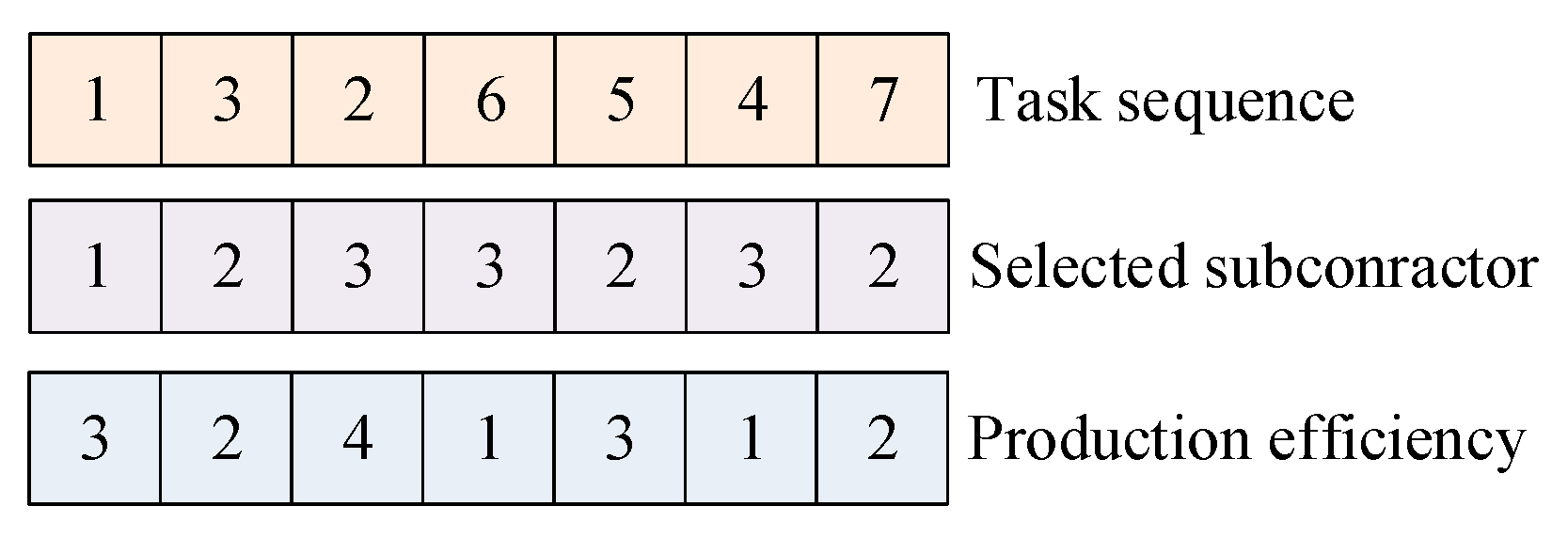
$y_{ij}^l$	Production efficiency, representing the variable resource input per unit of time
Objective Function
$F{T}_i$	The final time of project $P_i$
$d{p}_i$	The delay penalty for project $P_i$
${\mathrm{C}}_i\left(R\right)$	The resources cost of $P_i$
$F{C}_i$	Total cost of project $P_i$
$F{Q}_i$	Total quality of project $P_i$

Suppose that there are $n$ complex shipbuilding projects $\left\{P_1,\dots ,P_i,\dots ,P_n\right\}$ to be completed. According to the shipbuilding order contract, project $P_i$ should be completed before the delivery date $de{l}_i$. Each project is decomposed into a set of tasks. The tasks inside one project are constrained by the predecessor–successor relationship; otherwise, they are independent. Let us assume that $P_i$ contains $n_i$ tasks $\left\{T_{i1},T_{i2},\dots ,T_{ij},\dots ,T_{i{n}_i}\right\}$. The total workload of task $T_{ij}$ is marked as $Loa{d}_{ij}$ and the predecessor task group of $T_{ij}$ is marked as $PT{G}_{ij}$. Task $T_{ij}$ cannot start until all the predecessor tasks ($T_{ih}\in PT{G}_{ij}$) are fulfilled. In order to deal with the planning and scheduling problem, two virtual tasks $T_{i0}$ and $T_{i\left(n_i+1\right)}$ with the duration of zero are added as the start and end of $P_i$.

Let us consider that there are $m$ qualified cooperative enterprises $\left\{E_1,\dots ,E_l,\dots ,E_m\right\}$ having the production capacity to satisfy these task requirements. Each enterprise $E_l$ owns $m_l$ types of available resources $\left\{R_1^l,\dots ,R_k^l,\dots ,R_{m_l}^l\right\}$, among which the first $v_l$ types $R_k^l\left(k=1,\dots ,v_l\right)$ are the variable resources and the other $f_l$ types $R_k^l\left(k=v_l+1,\dots ,v_l+f_l\right)$ are the fixed resources. Using $a_k^l$ represents the available amount of resource $R_k^l$ per unit time, and $c_{kt}^l$ is the corresponding resource use cost at time $t$. Enterprises who are able to satisfy the production capacity requirements of task $T_{ij}$ constitute the group of candidate subcontractors marked as $CS{G}_{ij}$. The production capacity of these candidate subcontractors comes from the combination of resources they own. For example, enterprise $E_l\left(E_l\in CS{G}_{ij}\right)$ could fulfill the task $T_{ij}$ by using combinatorial resources. Let us define the minimum resource inputs as $ure{s}_{ij}^l=\left\{u{a}_{ij1}^l,\dots ,u{a}_{ijk}^l,\dots ,u{a}_{ij{m}_l}^l\right\}$, and the corresponding combination capacity is $Cap{a}_{ij}^l$, representing the accomplished workload with the consumption of resources $ure{s}_{ij}^l$ per unit of time.

Project planning and scheduling is used to choose the subcontractor and formulate the scheduling scheme for the tasks according to the task requirement and the capacity of each subcontractor. A candidate scheme of task $T_{ij}$ can be represented as $\left\{T_{ij},E_l,du{r}_{ij}^l ,s{t}_{ij}^l,q_{ij}^l\right\}$, where $T_{ij}$ is the task code, $E_l$ is the subcontractor code, $du{r}_{ij}^l$ is the duration, $s{t}_{ij}^l$ is the start time, and $q_{ij}^l$ is the completion quality. Based on the feature analysis, we can know:

(1)

If task $T_{ij}$ completed by enterprise $E_l$, the quality $q_{ij}^l$ is constant;

(2)

The task duration $du{r}_{ij}^l$ is affected by the inputs of the resource, which is up to subcontractor $E_l$ to negotiate with the general contractor;

(3)

The start time $s{t}_{ij}^l$ is later than the end time of the predecessor tasks.

Let us assume that if task $T_{ij}$ is completed by enterprise $E_l$, $T_{ij}$ occupies $re{s}_{ij}^l=\left\{a_{ij1}^l,\dots ,a_{ijk}^l,\dots ,a_{ij{m}_l}^l\right\}$ of the resources per unit of time in one scheduling scheme. The total resource input of task $T_{ij}$ is a combination of the variable resources $re{s}_{ij}^{lv}=\left\{a_{ijk}^l|k=1,\dots ,v_l\right\}$ and the fixed resources $re{s}_{ij}^{lf}=\left\{a_{ijk}^l|k=v_l+1,\dots ,v_l+f_l\right\}$. The occupied amount of fixed resources $a_{ijk}^l\left(k=v_l+1,\dots ,v_l+f_l\right)$ is constant in different scheduling schemes, and $a_{ijk}^l$ is equal to $u{a}_{ijk}^l$, while the occupied amount of variable resources $a_{ijk}^l\left(k=1,\dots ,v_l\right)$ varies from one scheduling scheme to another, and $a_{ijk}^l$ is a multiple of $u{a}_{ijk}^l$. Since the resources must be used in combination, we use a decision variable $y_{ij}^l$ to represent the resource inputs and production efficiency for different scheduling schemes.

$$a_{ijk}^l=\{\begin{array}{c}{y}_{ij}^l\ast u{a}_{ijk}^l, k=1,\dots ,v_l\\ u{a}_{ijk}^l, k=v_l+1,\dots ,v_l+f_l\end{array}$$

(1)

Since $a_{ijk}^l$ cannot exceed the total available amount $a_k^l$, the range of variable $y_{ij}^l$ is $\left\{1,2,\dots ,\lfloor \frac{a_k^l}{u{a}_{ijk}^l}\rfloor ; k=1,\dots ,v_l\right\}$. The duration is inversely proportional to the variable resource inputs. Normally, the duration $du{r}_{ij}^l$ can be calculated based on the variable $y_{ij}^l$.

$$du{r}_{ij}^l=\frac{Loa{d}_{ij}}{y_{ij}^l\ast Cap{a}_{ij}^l}$$

(2)

Obviously, the duration $du{r}_{ij}^l$ is not always an integer based on this Formula (2), which is inconsistent with the practical situation of the shipbuilding project. So, we rectify the formula as follows.

$$du{r}_{ij}^l=\lceil \frac{Loa{d}_{ij}}{y_{ij}^l\ast Cap{a}_{ij}^l}\rceil ,k=1,\dots ,v_l$$

(3)

The earliest and the latest finish time window $\left[E{F}_{ij}, L{F}_{ij}\right]$ of task $T_{ij}$ can be calculated by the traditional time calculation method in accordance with the operation logic of predecessor–successor tasks, the candidate completion scheme, and the project delivery date. The project planning scheme is an integration of all the task scheduling schemes. We set decision variable $x_{ijt}^l$ representing the end time of each task by a certain subcontractor. The final time of project $P_i$ can be calculated as Equation (4).

$$F{T}_i={\displaystyle \sum }_{t=E{F}_{i\left(n_i+1\right)}}^{L{F}_{i\left(n_i+1\right)}}{x}_{i\left(n_i+1\right)t}^1\ast t$$

(4)

In fact, shipbuilding contracts generally specify a deadline for delivery $dde{l}_i$ and a fine coefficient ${\theta }_i$ for the delivery delay. In other words, project $P_i$ is allowed to complete in time window $\left[1,dde{l}_i\right]$ in practical terms. The project time slot is $t=1,\dots ,dde{l}_i$. The optimal project completion time should be neither too early nor too late. This is because the contract prescribes the delivery date, and even though the project is completed earlier, the key fixed resources (e.g., docks) would not be released until the delivery, thus bringing no extra benefits. Considering that there is a trade-off between the delay penalty and the benefit brought by optimal resource utilization, the total project cost consists of the use cost of resources and the delay penalty. Formula (5) calculates the penalty for project delay, while Formula (6) calculates the costs of resources.

$$d{p}_i=\{\begin{array}{c}0,F{T}_i\le de{l}_i\\ {\theta }_i\ast \left(F{T}_i-de{l}_i\right), de{l}_i<F{T}_i\le dde{l}_i\end{array}$$

(5)

$${\mathrm{C}}_i\left(R\right)={\displaystyle \sum }_{j=1}^{n_i}{\displaystyle \sum }_{E_l\in CS{G}_{ij}}{\displaystyle \sum }_{t=E{F}_{ij}}^{L{F}_{ij}}{x}_{ijt}^l\ast {\displaystyle \sum }_{q=t-du{r}_{ij}^l+1}^t{\displaystyle \sum }_{k=v_l+1}^{m_l}{a}_{ijk}^l\ast c_{kq}^l$$

(6)

For each project, the overall objective is twofold: decreasing the cost and increasing the quality. So, the objective function is:

$$minF{C}_i={\mathrm{C}}_i\left(R\right)+d{p}_i$$

(7)

$$maxF{Q}_i={{\displaystyle \sum }}_{j=1}^{n_i}{{\displaystyle \sum }}_{E_l\in CS{G}_{ij}}{{\displaystyle \sum }}_{t=E{F}_{ij}}^{L{F}_{ij}}{x}_{ijt}^l\ast q_{ij}^l.$$

(8)

The constraints are:

$${\displaystyle \sum }_{E_l\in CS{G}_{ij}}{\displaystyle \sum }_{t=E{F}_{ij}}^{L{F}_{ij}}{x}_{ijt}^l=1,\forall i,j$$

(9)

$${\displaystyle \sum }_{E_l\in CS{G}_{ih}}{\displaystyle \sum }_{t=E{F}_{ih}}^{L{F}_{ih}}{x}_{iht}^l\ast t\le {\displaystyle \sum }_{E_l\in CS{G}_{ij}}{\displaystyle \sum }_{t=E{F}_{ij}}^{L{F}_{ij}}{x}_{ijt}^l\ast \left(t-du{r}_{ij}^l\right),\forall T_{ih}\in PT{G}_{ij},\forall i,j$$

(10)

$${\displaystyle \sum }_{j=1}^{n_i}{a}_{ijk}^l\ast {\displaystyle \sum }_{s=t}^{t+du{r}_{ij}^l-1}{x}_{ijt}^l\le a_k^l,\forall t,l,k$$

(11)

$$x_{ijt}^l\in \left\{0,1\right\},t=E{F}_{ij},\dots ,L{F}_{ij},\forall i,j,l$$

(12)

$$y_{ij}^l\in \left\{1,\dots ,\lfloor \frac{a_k^l}{u{a}_{ijk}^{lv}}\rfloor \right\},\forall i,j,l;k=1,2,\dots ,v_l$$

(13)

$$F{T}_i\le dde{l}_i.$$

(14)

Constraint (9) denotes that only one subcontractor is assigned to a task. Constraint (10) indicates that the task can be implemented after the completion of all predecessors. Constraint (11) is the total amount of constraints of all the resources. Constraints (12) and (13) represent the value range of the variables. Constraint (14) indicates that the completion date of the project must be before the specified deadline.

For each project $P_i$, the optimal solution ${\left(F{C}_i,F{Q}_i\right)}^{\ast }$ can be obtained by solving the above problem model, and then an optimal project planning scheme can be obtained based on the scheduling algorithm provided in Section 4.3. However, this scheme is merely based on the local needs of an individual project. Due to the total resource constraints of each subcontractor, the resource requests for each project may conflict. In this regard, all the project planning schemes must satisfy the resource constraints:

$${{\displaystyle \sum }}_{i=1}^n{{\displaystyle \sum }}_{j=1}^{n_i}{a}_{ijk}^l\ast {{\displaystyle \sum }}_{s=t}^{t+du{r}_{ij}^l-1}{x}_{ijt}^l\le a_k^l,\forall t,l,k.$$

(15)

The resource schemes for each project are local decisions, so Constraint (15) is usually unsatisfactory. It requires negotiation among projects to reasonably allocate manufacturing resources, which makes the planning scheme of these projects feasible. In order to realize it, a negotiation method is provided.

4.2.2. Iterative Combinational Auction-Based Negotiation Method

The project planning module adopts an iterative combinational auction mechanism to coordinate the resources usage among projects. The resource use rights of each subcontractor at time $t$ ($t=1,\dots ,T; T=\max \left(dde{l}_i\right), \forall p_i$) are regarded as the auction items. Subcontractor agents send the information of resource prices ($\mathsf{\Psi }=\left\{\partial \left(l,k,t\right):l=1,\dots ,m;k=1,\dots ,m_l;t=1,\dots ,T\right\}$ set by ${\mathrm{SA}}_l$, representing the price of resource $R_k^l$) to the auctioneer (combinational auction mechanism). In each iteration, an auctioneer communicates to the project agents (PAs) the current price of all the resources and receives the bids. The combinational auction process includes the following steps:

Step 1. Auctioneer initializes resource prices $\mathsf{\Psi }=\left\{\partial \left(l,k,t\right):l=1,\dots ,m;k=1,\dots ,m_l;t=1,\dots ,T\right\}$. Project agents (PAs) are informed the current price of resources.

Step 2. Project agents (PAs) build bids (${\mathsf{\Omega }}_i=\left\{{\rho }_i\left(l,k,t\right):l=1,\dots ,m;k=1,\dots ,m_l;t=1,\dots ,T\right\}$ set by ${\mathrm{PA}}_i$, representing the resource use amount requested by project $P_i$) according to the current price of auction items and communicate the bids to auctioneer to solve the problem of selecting subcontractors for each task and determining the start/finish time.

The bid ${\mathsf{\Omega }}_i=\left\{{\rho }_i\left(l,k,t\right):l=1,\dots ,m;k=1,\dots ,m_l;t=1,\dots ,T\right\}$ is a summary of the resource use scheme of all tasks in the local optimal solution, which can be calculated out as follows:

$${\rho }_i\left(l,k,t\right)={{\displaystyle \sum }}_{j=1}^{n_i}{a}_{ijk}^l\ast {{\displaystyle \sum }}_{s=t}^{t+du{r}_{ij}^l-1}{x}_{ijt}^l.$$

(16)

Project agent ${\mathrm{PA}}_i$ generates a completion scheme for each task in the task scheduling module. The scheduling process is to choose the subcontractor for the task and determine a feasible scheduling scheme, including the duration and the start time of each task according to the logical constraints between the tasks and the capacity of each subcontractor. Taking $T_{ij}$ as the example, a scheduling scheme is $pla{n}_{ij}=\left\{T_{ij},E_l,y_{ij}^l,s{t}_{ij}^l\right\}$ where $T_{ij}$ is the task code, $E_l$ is the selected subcontractor, $y_{ij}^l$ is the selected production efficiency to determine the duration, and $s{t}_{ij}^l$ is the start time. Based on $pla{n}_{ij}$, ${\rho }_{ij}\left(l,k,t\right)$ can be calculated out (the resource use amount requested by task $T_{ij}$). Correspondingly, the whole project plan $pla{n}_i$ is the combination of all the task completion schemes $\left\{pla{n}_{ij},j=1,\dots ,n_i\right\}$, i.e., ${\rho }_i\left(l,k,t\right)={{\displaystyle \sum }}_{j=1}^{n_i}{\rho }_{ij}\left(l,k,t\right)$. Current resource prices are $\mathsf{\Psi }=\left\{\partial \left(l,k,t\right):l=1,\dots ,m;k=1,\dots ,m_l;t=1,\dots ,T\right\}$; hence, the bid price $B_i\left({\mathsf{\Omega }}_i,\mathsf{\Psi }\right)$ of ${\mathrm{PA}}_i$ is the use cost of resources in the optimal solution.

Step 3. The auctioneer calculates revenue according to the bids and checks the resource conflicts. If there are no resource conflicts, the auction will be terminated.

For subcontractor agent (SAs), the local goal is to maximize the total revenue by allocating its available resources to the participating projects reasonably. On receipt of the bids from PAs, the auctioneer calculates and sends the resource request information to the corresponding SA. The calculation formula for the total resource requests to ${\mathrm{SA}}_l$ is as follows:

$$R_l\left(k,t\right)={{\displaystyle \sum }}_{i=1}^n{\rho }_i\left(l,k,t\right).$$

(17)

The total resource requests to ${\mathrm{SA}}_l$ should meet the total resource constraints $R_l\left(k,t\right)\le a_k^l$, which is another form of constraint (15). If there are no resource conflicts in an iteration, it indicates that all the requests can been met, and the auction will be terminated.

Step 4. Update the price of the auction items, turn to step 2, and start the next round of the auction.

Update the prices of resources by increasing the price of conflict resources and reducing the price of idle resources to resolve resource conflicts and guide PAs to use idle resources. Based on this principle, the auctioneer updates the resource prices $\mathsf{\Psi }=\left\{\partial \left(l,k,t\right):l=1,\dots ,m;k=1,\dots ,m_l;t=1,\dots ,T\right\}$ with consideration of the deviation $de{v}_l\left(k,t\right)=R_l\left(k,t\right)-a_k^l$, and by increasing the current value if $de{v}_l\left(k,t\right)>0$ (resource conflict) or decreasing it (at most to 0) if $de{v}_l\left(k,t\right)<0$ (idle resource).

The value of the increase (decrease) of ${\partial }^l\left(k,t\right)$ should be a non-decreasing (non-decreasing) function of excess (deficit); moreover, it is a good practice for auctioneers to actively obtain a good resource allocation in early iterations, while smaller adjustments can be made in later iterations to improve the same quality. This paper uses an algorithm inspired by the subgradient technique to update the price. At iteration $r$, the deviation of the resource requests is $de{v}_l^r\left(k,t\right)$, and let ${\mathsf{\Psi }}^{l,r}={\left\{{\partial }^{l,r}\left(k,t\right)\right\}}_{m_l\times T}$ be the matrix of the resource prices in which ${\partial }^{l,r}\left(k,t\right)$ is the price of resource $R_k^l$ in time period $t$. The new price of resource $R_k^l$ in time period $t$ at iteration $r+1$ is:

$${\partial }^{l,r+1}\left(k,t\right)=max\left\{0,{\partial }^{l,r}\left(k,t\right)+s^r\ast \frac{de{v}_l^r\left(k,t\right)}{{{\displaystyle \sum }}_{t=1}^T{\left(de{v}_l^r\left(k,t\right)\right)}^2}\right\}$$

(18)

where $s^r$ is a scalar controlling the aggressiveness of the auctioneer. The initial value of $s^r$ is $s^0$ and halves its value within a certain number of iterations:

$$s^{r+1}=max\left\{\frac{s^r}{2},0\right\}.$$

(19)

4.3. Task Scheduling Module

The project scheduling agent ($\mathrm{PSA}$) provides decision-making support for the project agent ($\mathrm{PA}$). The scheduling model of the research is designed to handle the problem of scheduling for distributed manufacturing resources. In each iteration, project agent (${\mathrm{PA}}_i$) generates a completion scheme for each task to obtain the optimal solution ${\left(F{C}_i,F{Q}_i\right)}^{\ast }$ for project $P_i$. The scheduling process is to choose the subcontractor for the tasks and determine a feasible scheduling scheme including the duration and the start time of each task.

The non-dominated sorting genetic algorithm (NSGA)-II has been proved to be one of the most effective methods to solve multi-objective problems [65,66,67,68,69,70]. However, due to the large work amount of complex shipbuilding projects, the length of coding increases, resulting in a huge solution space of the whole problem. Besides, because the elitism strategy has to compare every individual in the Pareto solution set, the calculation efficiency becomes rather low. Although the rate of crossover and variation can protect the diversity of population to a certain degree, the change of a genetic locus will greatly destroy the formed optimal Pareto solution set since that chromosome contains multiple types of characteristic information. Therefore, the traditional NSGA-II is difficult to obtain the global optimal solution. Correspondingly, the multi-agent genetic algorithm (MAGA), a technology based on artificial intelligence and an evolutionary algorithm, has strong local search capacity [71]. MAGA is a type of evolutionary algorithms for large-scale global numerical optimization. Due to the emphasis on local relations between the agents, the local search capacity of MAGA is very strong. Integrating the ideas of NSGA-II and MAGA, a non-dominated sorting multi-agent genetic algorithm (NSMAGA) with strong global and local search ability is used to solve the local project scheduling problem of this paper. The algorithm flowchart of NSMAGA is as shown in Figure 4.

4.3.1. Encoding and Decoding

For simplicity, the project number is omitted, and the problem is transformed into a single project scheduling problem. Design a triplet $1\times n$ matrix to express the feasible solution of the problem, where $n$ is the total number of tasks. The triplet matrix describes three characteristics of the project scheduling scheme: task sequence, selected subcontractor, and production efficiency. Figure 5 shows a feasible coding for a project scheduling example with seven tasks.

The first part of the solution describes the ordered list of the tasks that shows the order of the tasks’ entrance in the scheduling process. In this example, Figure 5 shows that Task 3 is the second task in the list of order of the tasks; in other words, Task 3 is the second task that should be scheduled. It is important to note that this task can be started only when all of its predecessors are finished and enough resources are available for executing it; otherwise, the next task in the list of order of the tasks should be considered. The second part of the solution represents the respective selected subcontractors of the task in the first part. In the discussion of this paper, the tasks are allocated to the qualified subcontractors with the production capacities required by the projects. In this example, Subcontractors 2 and 3 are the qualified subcontractors of Task 3, and Task 3 is assigned to Subcontractor 2. The third part of the solution depicts the selected production efficiency and resource inputs, i.e., the scheduling scheme with the multiplier of resource input. For each task, the duration can be obtained by a combination of the selected subcontractor and production efficiency.

Due to the structure of the solution matrix including the scheduling sequence, subcontractor, and production efficiency, the scheduling scheme can be generated by determining the start time $\left\{{\mathrm{s}}_1,{\mathrm{s}}_2,\dots ,{\mathrm{s}}_{\mathrm{n}}\right\}$. For one solution matrix, the project quality $FQ$ is constant. So, the decoding rule is applied to generate the optimal schedule corresponding to minimum project cost $\left(\min FC\right)$. To describe the decoding rule more clearly, it is necessary to add some notations:

$US$	the unscheduled task matrix order by the scheduling sequence
$PS$	the scheduled task matrix
${\mathrm{j}}^{\ast }$	the task with premier order in matrix $US$
${\mathrm{p}}_{\mathrm{j}}$	the predecessor group of task $\mathrm{j}$
${\mathrm{ES}}_{\mathrm{j}}$	the earliest start time of task $\mathrm{j}$
${\mathrm{EF}}_{\mathrm{j}}$	the earliest finish time of task $\mathrm{j}$
${\mathrm{LS}}_{\mathrm{j}}$	the latest start time of task $\mathrm{j}$
${\mathrm{LF}}_{\mathrm{j}}$	the latest finish time of task $\mathrm{j}$
${\mathrm{s}}_{\mathrm{j}}$	the start time of task j
${\mathrm{f}}_{\mathrm{j}}$	the finish time of task j
${\mathrm{A}}_{\mathrm{j}}$	the order of task j
${\mathrm{M}}_{\mathrm{j}}$	the selected subcontractor of task j
$\mathrm{d}\left(\mathrm{j}\right)$	the duration of task j
$\mathrm{r}\left(\mathrm{j}\right)$	the resource requirement of task j

Obviously, the optimal solution can be obtained by iterating through the scope of the solution space ($s_i\in \left[0,deadline\right]$), which works, but takes a lot of time. Consequently, it is necessary to narrow the scope of the solution space by preprocessing the constraints.

In order to narrow the scope of the solution space, two rounds of scheduling are carried out to obtain the earliest and latest start time of each task. The scheduling process of the tasks is divided into “n stages”, while one task is scheduled in each stage. The first task in the scheduling sequence that has no predecessors will be scheduled in the first stage. Then, the other tasks based on their location in the scheduling sequence will be scheduled in the next stages. In each stage, all tasks whose predecessors are finished completely are placed at the matrix ($US$) firstly, and task (${\mathrm{j}}^{\ast }$) with a premier order amongst other tasks in the scheduling sequence will be selected to schedule in this stage. For task (${\mathrm{j}}^{\ast }$), its earliest start time (${\mathrm{ES}}_{{\mathrm{j}}^{\ast }}$) will be calculated out in two steps. Firstly, the logical relationships between tasks are considered. The task’s ${\mathrm{ES}}_{{\mathrm{j}}^{\ast }}$ equals the maximum finish times ($max\left\{{\mathrm{ES}}_{\mathrm{h}}+{\mathrm{d}}_{\mathrm{h}}\right\}$) of its predecessors ($\mathrm{h}\in {\mathrm{p}}_{\mathrm{j}}$). If there is no predecessor, the task’s ${\mathrm{ES}}_{{\mathrm{j}}^{\ast }}$ is equal to zero (the outset of the scheduling time horizon). Secondly, check the resource constraints. If the resources conflict, delay the earliest start time (${\mathrm{ES}}_{{\mathrm{j}}^{\ast }}$) by one unit repeatedly until the resource constraints are satisfied. The scheduled tasks will be moved to the matrix ($PS$) from the matrix ($US$). Similarly, the latest start time (${\mathrm{LS}}_{\mathrm{j}}$) of each task can be calculated out by reverse scheduling the tasks in matrix ($PS$) and setting the value of deadline to the finish time of the last task. Then, iterate through the scope of the solution space (${\mathrm{s}}_{\mathrm{j}}\in \left[{\mathrm{ES}}_{\mathrm{j}},{\mathrm{LS}}_{\mathrm{j}}\right]$) to obtain the optimal schedule ${\left\{{\mathrm{s}}_1,{\mathrm{s}}_2,\dots ,{\mathrm{s}}_{\mathrm{n}}\right\}}^{\ast }$. The schedule corresponding to the minimum project cost is the solution of start times added to the solution matrix. The decoding process can be summarized and explained procedurally as follows:

Algorithm 1: Schedule Generation

Step 1. Insert into the solution matrix: sequence, subcontractor, and production efficiency of all tasks. Step 2. Calculate $\mathrm{d}\left(\mathrm{j}\right), \mathrm{r}\left(\mathrm{j}\right)$ for each task. Step 3. Calculate the earliest start times of each task. Step 3.1. $PS=\varnothing ,\mathrm{ns}=1$. Step 3.2. $US=\left\{\mathrm{j}|\mathrm{j}\notin PS, {\mathrm{p}}_{\mathrm{j}}\in PS\right\}$. Step 3.3. ${\mathrm{j}}^{\ast }=j|\max \left\{priority\left(j\right)\right\},\mathrm{j}\in US$. Step 3.4. $\mathrm{ES}\left({\mathrm{j}}^{\ast }\right)=\max \{0,\max \{f\left(h\right)|h\in p\left({\mathrm{j}}^{\ast }\right)\}\}$. Step 3.5. $\mathrm{s}\left({\mathrm{j}}^{\ast }\right)=\mathrm{ES}\left({\mathrm{j}}^{\ast }\right)$. Step 3.6. $\mathrm{Available}\mathrm{resource}\left(\mathrm{k},\mathrm{t}\right)=\mathrm{resource}\left(\mathrm{k},\mathrm{t}\right)-\sum \mathrm{r}\left(\mathrm{j}\right),j\in PS,t\in \left[\mathrm{s}\left({\mathrm{j}}^{\ast }\right),\mathrm{s}\left({\mathrm{j}}^{\ast }\right)+\mathrm{d}\left({\mathrm{j}}^{\ast }\right)\right]$. Step 3.7. If $\mathrm{r}\left({\mathrm{j}}^{\ast }\right)>\mathrm{Available}\mathrm{resource}\left(\mathrm{k},\mathrm{t}\right),\mathrm{s}\left({\mathrm{j}}^{\ast }\right)=\mathrm{s}\left({\mathrm{j}}^{\ast }\right)+1$, go to Step 3.6. Step 3.8. $\mathrm{ES}\left({\mathrm{j}}^{\ast }\right)=\mathrm{s}\left({\mathrm{j}}^{\ast }\right)$. Step 3.9. $PS=PS\cup \left\{{\mathrm{j}}^{\ast }\right\},ns=ns+1$. Step 3.10. If $ns\le n$, go to Step 3.2. Step 4. Calculate the latest start times of each task. Step 4.1. $P{S}_2=\varnothing ,ns=1$. Step 4.2. ${\mathrm{j}}^{\ast }=j|\max \left\{location\left(PS\right),\mathrm{j}\notin P{S}_2\right\}$. Step 4.3. $\mathrm{LS}\left({\mathrm{j}}^{\ast }\right)=\min \left\{deadline,\min \left\{s\left(h\right){|\mathrm{j}}^{\ast }\in p\left(h\right)\right\}\right\}-\mathrm{d}\left({\mathrm{j}}^{\ast }\right)$. Step 4.4. $\mathrm{s}\left({\mathrm{j}}^{\ast }\right)=\mathrm{LS}\left({\mathrm{j}}^{\ast }\right)$. Step 4.5. $\mathrm{Available}\mathrm{resource}\left(\mathrm{k},\mathrm{t}\right)=\mathrm{resource}\left(\mathrm{k},\mathrm{t}\right)-\sum \mathrm{r}\left(\mathrm{j}\right),j\in PS,t\in \left[\mathrm{s}\left({\mathrm{j}}^{\ast }\right),\mathrm{s}\left({\mathrm{j}}^{\ast }\right)+\mathrm{d}\left({\mathrm{j}}^{\ast }\right)\right]$. Step 4.6. If $\mathrm{r}\left({\mathrm{j}}^{\ast }\right)>\mathrm{Available}\mathrm{resource}\left(\mathrm{k},\mathrm{t}\right),\mathrm{s}\left({\mathrm{j}}^{\ast }\right)=\mathrm{s}\left({\mathrm{j}}^{\ast }\right)-1$, go to Step 4.5. Step 4.7. $\mathrm{LS}\left({\mathrm{j}}^{\ast }\right)=\mathrm{s}\left({\mathrm{j}}^{\ast }\right)$. Step 4.8. $P{S}_2=P{S}_2\cup \left\{{\mathrm{j}}^{\ast }\right\},ns=ns+1$. Step 4.9. If $ns\le n$, go to Step 4.2. Step 5. Iterate through the scope of solution space (${\mathrm{s}}_{\mathrm{j}}\in \left[{\mathrm{ES}}_{\mathrm{j}},{\mathrm{LS}}_{\mathrm{j}}\right]$) to obtain the optimal schedule $\left({\mathrm{s}}_1,{\mathrm{s}}_2,\dots ,{\mathrm{s}}_{\mathrm{n}}\right)$.

4.3.2. Initialize the Population

In the proposed algorithm, each individual in the population is regarded as an agent representing a candidate solution of the optimization problem. An agent is expressed as $a=\left\{body, energy, neighborhood\right\}$, where $body$ represents the coding of a solution, $energy$ is equal to the value of the objective function {$FQ,FC$}, and $neighborhood=\left\{N_1, N_2, \dots ,N_k\right\}$ is the neighborhood of $a$ where $N_i=\left(b, trustdegree\left(a,b\right)\right)$ represents the relation between $a$ and $b$, $trustdegree\left(a,b\right)$ is the trust degree between $a$ and $b$, and the range of $trustdegree$ is [−1, 1]. The neighborhood of $a$ changes as the $trustdegree$ changes. According to human society, the neighborhood being extended and reduced follows the modes:

Extended mode: Randomly select an agent $b$ from the network outside of the neighborhood of $a$, place $b$ into the neighborhood of $a$, and set $trustdegree\left(a,b\right)$ = 0; if agent $b$ is in the neighborhood of $a_{ij}$ and $trustdegree\left(a,b\right)=1$, and agent $c$ is in the neighborhood of $b$ and $trustdegree\left(b,c\right)=1$, place $c$ into the neighborhood of $a$ and set $trustdegree\left(a,b\right)=1$.

Cut mode: If agent $b$ is in the neighborhood of $a$ and $trustdegree\left(a,b\right)=-1$, take $b$ out of the neighborhood of $a$.

An agent exists in a network with the size of ($La\times La$). In order to prevent the boundary effect, the network topology is the ring. Suppose that the population size is $N$, the Pareto solution set is $P_{best}$ with the size of $\overline{N}$, and the maximum number of evolutionary iterations is ${\mathrm{g}}_{max}$. Randomly generate $N$ ($N=La\times La$) individuals as the initial population based on the coding rules and place these individuals in the agent network. Agent $a_{ij}$ represents the individual in position $\left(i, j\right)$ of the network. The energy of each agent can be obtained based on the schedule generation algorithm. The initial neighborhood of each agent contains only four agents in the adjacent location, and the initial $trustdegree$ is zero. For agent $a_{ij}$, the initial neighborhood is $neighborhood=\left\{\left(a_{i^{\prime }j},0\right), \left(a_{i{j}^{\prime }},0\right),\left(a_{i^{″}j},0\right), \left(a_{i{j}^{″}},0\right)\right\}$, where $i^{\prime }=\{\begin{array}{c}i-1, i\ne 1\\ La, i=1\end{array}$, $j^{\prime }=\{\begin{array}{c}j-1, j\ne 1\\ La, j=1\end{array}$, $i^{″}=\{\begin{array}{c}i+1, i\ne La\\ 1, i=La\end{array}$, $j^{″}=\{\begin{array}{c}j+1, j\ne La\\ 1, j=La\end{array}$.

4.3.3. Rapid Non-Dominated Sorting and Tournament Selection

When all the objective function values of populations are calculated out by the schedule generation algorithm, rapid non-dominated sorting is employed to module the current populations and give them corresponding serial numbers. The serial numbers of some individuals are the same. In terms of selection, crowding distance calculation is needed for the consideration of population diversity [72,73]. The energy of an agent with a smaller serial number and bigger crowding distance is considered larger. Tournament selection is used to choose the agent with larger energy when needed in the process of the algorithm. Firstly, comparing the corresponding serial numbers of the agents, we choose the agent with the smaller serial number. If there are several agents with the same serial numbers, we compare their corresponding crowding distances and choose the agent with the bigger crowding distance. In NSGA-II, the Pareto preferential should be carried out after non-dominated sorting if the size of the current population is beyond the initial value. NSGA-II solves this problem by comparing the crowding distance to successively select the individuals with the bigger crowding distances. This method could result in the distance between some individuals being too far, making the distribution of the individuals too sparse. For overcoming the shortcoming, this paper adapts other ways to carry out the Pareto preferential, which is to prune the individuals with smaller crowding distance successively until the size of the population is sufficient.

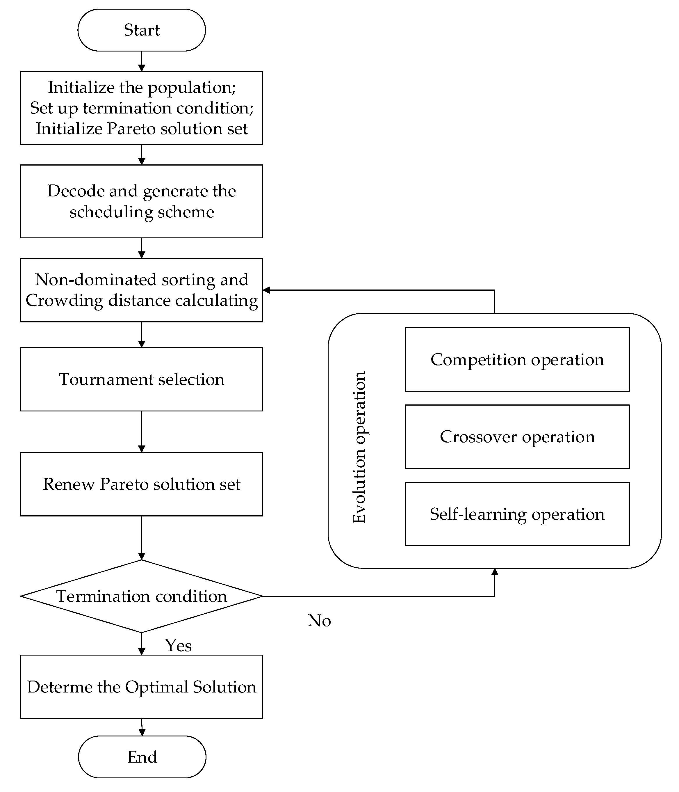
4.3.4. Evolution Operation

The evolutionary goal of the agent is to increase its energy (lower cost and higher quality). In the evolutionary process, each agent implements multiple evolution operations with certain probability.

● Competition operation

The competition operation occurs in the current agent $a$ by the occupied probability $P_o$. Through tournament selection, the agent $a_{max}$ is selected from the neighborhood. If the energy of $a$ is less than that of $a_{max}$, replace $a$ with $a_{max}$; else, keep $a$ unchanged.

Algorithm 2: Competition Operation

Step 1: Input agent $a$. The occupied probability $P_o$; Step 2: Generate random number $P\in \left(0,1\right)$. If $P\le P_o$, go to Step 3; else, go to Step 5; Step 3: Select agent $a_{max}$ with the maximum energy from the neighborhood of $a$ by tournament selection; Step 4: If the energy of $a$ is less than that of $a_{max}$, set $a.body=a_{max}.body$ and $a.energy=a_{max}.energy$; Step 5: Output agent $a$.

● Collaborative crossover

Collaborative crossover is the behavior between $a$ and $b$ that is selected to be the collaborative agent with the probability $Pc+trustdegree\left(a, b\right)\ast 0.1$ from the neighborhood of $a$. A binary random 0–1 array is to decide the crossover position, as shown in Figure 6. For the task sequence, if the value is “1” in binary array, keep the corresponding position of the offspring body unchanged, and then place the rest of the values from the collaborative agent $b$ into the remaining positions of the offspring body in order. For the selected subcontractor and production efficiency sequences, if the value is “1”, we should find the corresponding tasks of the positions. Then, place the corresponding subcontractors and efficiency of the tasks into the position of the task at the offspring body and place the value from the collaborative agent $b$ into the remaining position of the offspring body. So, we obtain an offspring agent $a^{\prime }$. Calculate the function values of $a^{\prime }$. If $a^{\prime }$ can dominate $a$, replace $a$ with $a^{\prime }$ and set $trustdegree\left(a, b\right)=trustdegree\left(a, b\right)+0.1$; else, set $trustdegree\left(a, b\right)=trustdegree\left(a, b\right)-0.2$.

Algorithm 3: Collaborative Crossover Operation

Step 1: Input agent $a$, the number of neighbors of $a$ is $J$; Step 2: The crossover probability $P_C$; Step 3: Initialize the agent $a^{\prime }=a$; $j=1$; Step 4: Set $\mathrm{b}=\mathrm{b}|N_j\left(b, trustdegree\right)$ from the neighborhood of $a$; Step 5: Generate random number $P\in \left(0,1\right)$. If $P\le Pc+trustdegree\ast 0.1$, go to Step 6; else, go to Step 8; Step 6: Generate the binary array and implement the collaborative crossover operation to get $a^{\prime }$; Step 7: If $a^{\prime }$ can dominate $a$, replace $a$ with $a^{\prime }$ and set $trustdegree\left(a, b\right)=trustdegree\left(a, b\right)+0.1$; ease if $a$ can dominate $a^{\prime }$, set $trustdegree\left(a, b\right)=trustdegree\left(a, b\right)-0.2$; else, neither can dominate $a^{\prime }$. Step 8: $j=j+1$, if $j\le J$, go to Step 4; else, go to Step 9; Step 9: Output agent a.

● Self-learning

Self-learning behavior improves the energy due to an agent’s own knowledge. For the task sequence, select two positions randomly, place the code in the first position into the second position, and place the other codes in order. For the selected subcontractor and production efficiency sequences, select one position randomly and find the corresponding task; then, change the value of the selected subcontractor and production efficiency to a random 1~M/P (M/P is the maximum value to be selected) and place the new value into the position of the corresponding task of $a^{\prime }$. An example of self-learning is shown in Figure 7. If $a^{\prime }$ can dominate $a$, replace $a$ with $a^{\prime }$.

Algorithm 4: Self-Learning Operation

Step 1: The self-learning probability $P_s$; Step 2: Generate the random number $P\in \left(0,1\right)$. If $P\le P_s$, go to Step 3; else, go to Step 8; Step 3: Choose the agent $a$ by tournament selection; the length of the code is $n$; Step 4: Initialize the agent $a\prime =a$; Step 5: Generate two numbers R1, R2 between (1, n − 1) randomly, then place the code in the position R1 into R2 and place the other codes in order; If $\mathrm{a}\prime$ can dominate a, replace $a$ with $a^{\prime }$; Step 6: Generate one number R3 between (1, n − 1) randomly, find the corresponding task, change the value of the selected subcontractor to a random 1~M, and place it into the position of the corresponding task of $\mathrm{a}\prime$ in the selected subcontractor sequence; If $a^{\prime }$ can dominate $a$, replace $a$ with $a^{\prime }$. Step 7: Generate one number R4 between (1, n − 1) randomly, find the corresponding task, change the value of production efficiency to a random 1~P and place it into the position of the corresponding task of $\mathrm{a}\prime$ in the production efficiency sequence; If $a^{\prime }$ can dominate $a$, replace $a$ with $a^{\prime }$. Step 8: Output agent a.

4.3.5. Determine the Optimal Scheme

After obtaining the Pareto solution set $P_{best}$, the optimal scheduling scheme still needs to be determined. Suppose that there are $p$ Pareto solutions $\left\{S_1,S_2,\dots ,S_p\right\}$, among which $S_e\in P_{best},e=1,\dots ,p.$ is a candidate scheme, the corresponding objective function values are $\left\{F{C}_e, F{Q}_e\right\}$, which can be regarded as the evaluation vector of scheme $S_e$. There are different optimum values from different decision-making angles. The entropy weight method and TOPSIS method have been proven to be an efficient way to select the optimal scheme [74,75,76,77]. Follow the following steps to evaluate the project:

(1) Let us define the evaluation matrix $A=\left[\begin{array}{c}{r}_{11}\\ r_{21}\end{array}\begin{array}{c}{r}_{12}\\ r_{22}\end{array}\begin{array}{c}\dots \\ \dots \end{array}\begin{array}{c}{r}_{1p}\\ r_{2p}\end{array}\right]$ based on the objective function values, where $\left\{r_{1e}, r_{2e}\right\}$ are two evaluation indexes corresponding to the cost and quality function values of solution $S_e$, respectively.

(2) For all the Pareto solutions, the minimum (maximum) cost and quality score are $\underset{e\in \left[1,p\right]}{\min } r_{ie}\left(\underset{e\in \left[1,p\right]}{\max } r_{ie}\right),i=1,2;e=1,\dots ,p$. Standardize matrix $A$ as Equation (20) to get matrix $B={\left\{b_{ie}\right\}}_{2\times p}$.

$$b_{ie}=\frac{r_{ie}-\underset{e\in \left[1,p\right]}{\min } r_{ie}}{\underset{e\in \left[1,p\right]}{\max } r_{ie}-\underset{e\in \left[1,p\right]}{\min } r_{ie}},i=1,2;e=1,\dots ,p$$

(20)

(3) Define the weighting coefficient of two objectives as $W=\left\{{\omega }_i\right|i=1,2\}$, which can be calculated as Equations (21)–(23).

$$f_{ie}=\frac{b_{ie}}{{{\displaystyle \sum }}_1^p{b}_{ie}},i=1,2;e=1,\dots ,p$$

(21)

$$E_i=-\ln {\left(p\right)}^{-1}{\displaystyle \sum }_{e=1}^p f_{ie}\times \ln f_{ie},i=1,2$$

(22)

$$w_i=\frac{1-E_i}{2-(E_1+E_2)}i=1,2$$

(23)

(4) Generate the weighted decision matrix $V$ by multiplying the standardized matrix $B$ and the weighting coefficient ${\omega }_i$ of each evaluation index.

$$V={\left\{v_{ie}\right\}}_{2\times p}=\left[\begin{array}{c}{b}_{11}\ast w_1\\ b_{21}\ast w_2\end{array} \begin{array}{c}{b}_{12}\ast w_1\\ b_{22}\ast w_2\end{array} \begin{array}{c}\dots \\ \dots \end{array} \begin{array}{c}{b}_{1p}\ast w_1\\ b_{2p}\ast w_2\end{array}\right]$$

(24)

(5) Calculate the positive and negative ideal solutions.

The optimal scheme $V^{+}=\left\{v_1^{+},v_2^{+}\right\}$ and the worst scheme $V^{-}=\left\{v_1^{-},v_2^{-}\right\}$ are determined in the weighted decision matrix, where $v_1^{+}=\underset{e\in \left[1,p\right]}{mix}{v}_{1e},v_2^{+}=\underset{e\in \left[1,p\right]}{max}{v}_{2e},v_1^{-}=\underset{e\in \left[1,p\right]}{max}{v}_{1e},v_2^{-}=\underset{e\in \left[1,p\right]}{mix}{v}_{2e}$.

(6) Calculate the Euclidean distance between the candidate scheme $S_e$ and the optimal scheme/the worst scheme.

$$D_e^{+}=\sqrt{{\left(v_1^{+}-v_{1e}\right)}^2+{\left(v_2^{+}-v_{2e}\right)}^2},e=1,\dots ,p$$

(25)

$$D_e^{-}=\sqrt{{\left(v_{1e}-v_1^{-}\right)}^2+{\left(v_{2e}-v_2^{-}\right)}^2},e=1,\dots ,p$$

(26)

(7) Calculate the approximation degree of the candidate scheme to the optimal one.

$$C_e=\frac{D_e^{-}}{D_e^{-}+D_e^{+}},e=1,\dots ,p$$

(27)

The larger value of approximation degree $C_e$ indicates that the scheme is closer to the optimal solution.

5. Experiment and Results Analysis

The proposed approach is implemented in a simulated manufacturing system. Simulations were performed on several Windows 10 operating systems with an Intel Core i7-6700 2.60 GHz processor and 8 GB of RAM to test the process of shipbuilding project planning and scheduling. Agent behaviors, protocols, and the scheduling algorithm were coded in MATLAB 2016b and collectively used to support the agent-based simulations.

In order to test the effectiveness of the proposed approach, an illustrative example is conducted. Due to the huge amount of shipbuilding project statistics, this article takes the plans corresponding to hull blocks as verification objects. For clear demonstration of the interactions among project participants, we consider a parallel planning problem with two projects $\left\{P_1,P_2\right\}$ and three cooperative enterprises $\left\{E_1,E_2,E_3\right\}$. Each project contains 36 tasks, respectively. Each cooperative enterprise owns two kinds of variable resources ($R_1\&R_2$) and fixed resources ($R_3\&R_4$) that are available, respectively.

Table 1. Information of projects and candidate subcontractors.

Project	Task	Workload	Predecessors	Candidate Scheme
				Enterprise	Quality	Resources
Project code: $P_1$ Complete windows: 2019.4.01–2019.5.20 Deadline: 2019.5.31 Fine coefficient: US$10,000	$T_1$	--	--	--	--	--
	$T_2$	10	$T_1$	$E_3$	6	0,2,2,0
	$T_3$	15	$T_1$	$E_1$	10	6,0,0,5
				$E_2$	3	0,10,5,0
				$E_3$	2	0,10,0,4
	$T_4$	14	$T_1$	$E_2$	5	3,0,8,0
	$T_5$	15	$T_2$,$T_4$	$E_3$	1	10,0,6,0
	$T_6$	15	$T_5$	$E_1$	7	9,0,0,8
				$E_2$	2	6,0,0,5
				$E_3$	6	0,2,0,5
	$T_7$	12	$T_4$	$E_3$	9	0,8,0,6
	…	…	…	…	…	…
	$T_{33}$	12	$T_{29}$	$E_1$	1	6,0,0,5
				$E_2$	8	8,0,10,0
				$E_3$	9	0,7,7,0
	$T_{34}$	14	$T_{30}$,$T_{32}$	$E_2$	1	10,0,6,0
	$T_{35}$	10	$T_{27}$,$T_{31}$	$E_1$	4	0,2,0,5
				$E_3$	8	0,5,5,0
	$T_{36}$	--	$T_{33}$,$T_{34}$,$T_{35}$	--	--	--
Project code: $P_2$ Complete windows: 2019.4.11–2019.5.30 Deadline: 2019.6.10 Fine coefficient: US$10,000	$T_1$	--	--	--	--	--
	$T_2$	14	$T_1$	$E_1$	6	6,0,0,1
				$E_2$	6	0,10,8,0
	$T_3$	10	$T_1$	$E_2$	8	0,10,5,0
				$E_3$	8	0,10,0,4
	$T_4$	15	$T_1$	$E_1$	4	3,0,0,7
				$E_2$	7	3,0,8,0
				$E_3$	3	3,0,0,3
	$T_5$	14	$T_2$,$T_4$	$E_2$	1	10,0,6,0
	$T_6$	12	$T_5$	$E_3$	6	0,2,0,5
	…	…	…	…	…	…
	$T_{33}$	10	$T_{29}$	$E_1$	2	6,0,0,5
				$E_2$	4	8,0,10,0
				$E_3$	6	0,7,7,0
	$T_{34}$	11	$T_{30}$,$T_{32}$	$E_1$	8	5,0,0,1
				$E_2$	1	0,7,10,0
				$E_3$	4	0,7,0,8
	$T_{35}$	13	$T_{27}$,$T_{31}$	$E_1$	6	0,2,5,0
	$T_{36}$	--	$T_{33}$,$T_{34}$,$T_{35}$	--	--	--

displays the detailed project information. Task $T_1$ and $T_{36}$ in each project are virtual tasks with the duration of zero, representing the start and end of each project. Task $T_2 \mathrm{to}{T}_{35}$ are real tasks. The basic information of each task include the workload, predecessors, and candidate scheme. Each task has several production schemes to choose from, which are provided by cooperative enterprises with different production capacities. The candidate scheme of each task includes the executive enterprise code, quality, and resources scheme (the minimum resource inputs $\left\{R_1,R_2,R_3,R_4\right\}$). Taking task $T_3$ in Project $P_1$ as an example, the workload is 15, the predecessor is $T_1$ and enterprises $E_1$, $E_2$, and $E_3$ all have the production capacity to satisfy the requirements of task $T_3$. If task $T_3$ is fulfilled by enterprise $E_1$, the quality is 10 and the minimum resource inputs are {6, 0, 0, 5}. Some tasks have multiple predecessors, such as task $T_5$. The daily supply capacity ($a_i, i=1,2,3,4$) and price ($c_i, i=1,2,3,4$) of each resource are shown in

Table 2. Available resource information of subcontractors.

Enterprise	${\mathit{R}}_1$		${\mathit{R}}_2$		${\mathit{R}}_3$		${\mathit{R}}_4$
	${\mathit{a}}_1$	${\mathit{c}}_1$	${\mathit{a}}_2$	${\mathit{c}}_2$	${\mathit{a}}_3$	${\mathit{c}}_3$	${\mathit{a}}_4$	${\mathit{c}}_4$
$E_1$	20	1000	23	1000	26	1000	36	1000
$E_2$	20	1000	23	1000	26	1000	36	1000
$E_3$	20	1000	23	1000	26	1000	36	1000

.

According to the negotiation strategy in Section 4.2.2, each project generates a completion scheme for each task by local scheduling in each iteration of a combinational auction. In the local decision-making process, NSMAGA is used to find an optimal solution for the best combination of cost and quality. The parameters of NSMAGA are listed as follows: the largest repetition number ${\mathrm{g}}_{max}$ is 100, the initial population size $N$ is 100, the agent network size $La$ is 10, the Pareto solution set size $\overline{N}$ is 50, the occupied probability $P_o$ is 0.9, the crossover probability $P_C$ is 0.9, and the self-learning probability $P_s$ is 0.1. After running the algorithm, the local scheduling optimal solution of each project can be obtained.

Table 3. Local scheduling results of project $P_1$ in one iteration.

Task	Subcontractor	Duration	Start Time	Start Time	Resources
$T_1$	--	0 days	2019/4/1	2019/4/1	--
$T_2$	$E_3$	5 days	2019/4/1	2019/4/6	0,16,8,0
$T_3$	$E_1$	5 days	2019/4/1	2019/4/6	18,0,0,5
$T_4$	$E_2$	2 days	2019/4/1	2019/4/3	15,0,8,0
$T_5$	$E_2$	5 days	2019/4/6	2019/4/11	20,0,6,0
$T_6$	$E_3$	2 days	2019/4/11	2019/4/13	0,16,0,5
$T_7$	$E_2$	5 days	2019/4/3	2019/4/8	0,24,0,6
$T_8$	$E_3$	5 days	2019/4/6	2019/4/11	15,0,3,0
$T_9$	$E_1$	2 days	2019/4/8	2019/4/10	18,0,0,7
$T_{10}$	$E_1$	6 days	2019/4/11	2019/4/17	0,20,0,5
$T_{11}$	$E_3$	4 days	2019/4/22	2019/4/26	0,9,6,0
$T_{12}$	$E_3$	4 days	2019/4/13	2019/4/17	0,18,2,0
$T_{13}$	$E_3$	4 days	2019/4/17	2019/4/21	0,21,0,2
$T_{14}$	$E_2$	5 days	2019/4/11	2019/4/16	6,0,6,0
$T_{15}$	$E_3$	4 days	2019/4/26	2019/4/30	18,0,0,5
$T_{16}$	$E_2$	4 days	2019/4/17	2019/4/21	0,21,0,8
$T_{17}$	$E_3$	1 day	2019/4/21	2019/4/22	0,26,5,0
$T_{18}$	$E_2$	3 days	2019/4/30	2019/5/3	5,0,0,0
$T_{19}$	$E_3$	6 days	2019/4/21	2019/4/27	2,0,0,0
$T_{20}$	$E_2$	4 days	2019/4/22	2019/4/26	18,0,0,1
$T_{21}$	$E_2$	12 days	2019/4/26	2019/5/8	6,0,0,5
$T_{22}$	$E_1$	2 days	2019/5/8	2019/5/10	18,0,0,3
$T_{23}$	$E_3$	6 days	2019/5/3	2019/5/9	20,0,6,0
$T_{24}$	$E_1$	4 days	2019/5/10	2019/5/14	0,8,0,5
$T_{25}$	$E_3$	5 days	2019/5/9	2019/5/14	0,16,0,6
$T_{26}$	$E_2$	7 days	2019/5/8	2019/5/15	16,0,0,6
$T_{27}$	$E_1$	2 days	2019/5/14	2019/5/16	16,0,0,6
$T_{28}$	$E_2$	6 days	2019/5/15	2019/5/21	0,20,0,5
$T_{29}$	$E_1$	4 days	2019/5/10	2019/5/14	0,9,6,0
$T_{30}$	$E_1$	6 days	2019/5/14	2019/5/20	0,12,2,0
$T_{31}$	$E_2$	3 days	2019/5/21	2019/5/24	10,0,0,5
$T_{32}$	$E_3$	3 days	2019/5/9	2019/5/12	15,0,6,0
$T_{33}$	$E_3$	4 days	2019/5/14	2019/5/18	0,21,7,0
$T_{34}$	$E_2$	5 days	2019/5/21	2019/5/26	0,14,10,0
$T_{35}$	$E_1$	2 days	2019/5/24	2019/5/26	0,18,5,0
$T_{36}$	--	0 days	2019/5/26	2019/5/26	--

shows the scheduling results of Project 1. The corresponding Gantt chart is shown in Figure 8.

Since the scheduling scheme of each project is a local optimal solution, resource conflicts are inevitable. Each subcontractor needs to update the prices of resources by increasing the price of conflict resources and reducing the price of idle resources to resolve resource conflicts and guide PAs to use idle resources. According to the update strategy of the resource prices in Section 4.2.2, the initial aggressiveness parameter $s^0$ needs to be set in advance. In this illustration, the parameter $s^0$ is set to 2. Figure 9, Figure 10, Figure 11 and Figure 12 shows the situation of resource request and conflicts for cooperative enterprises $\left\{E_1,E_2,E_3\right\}$ after 5, 10, 15, and 18 iterations. In the figures, the red line refers to the total amount of available resources. After 18 iterations, the resource conflicts are resolved, and all the resource requests of the two projects are met. In the distributed decision-making environment, the goal coordination of project participants is achieved. The results show that the proposed method is effective.

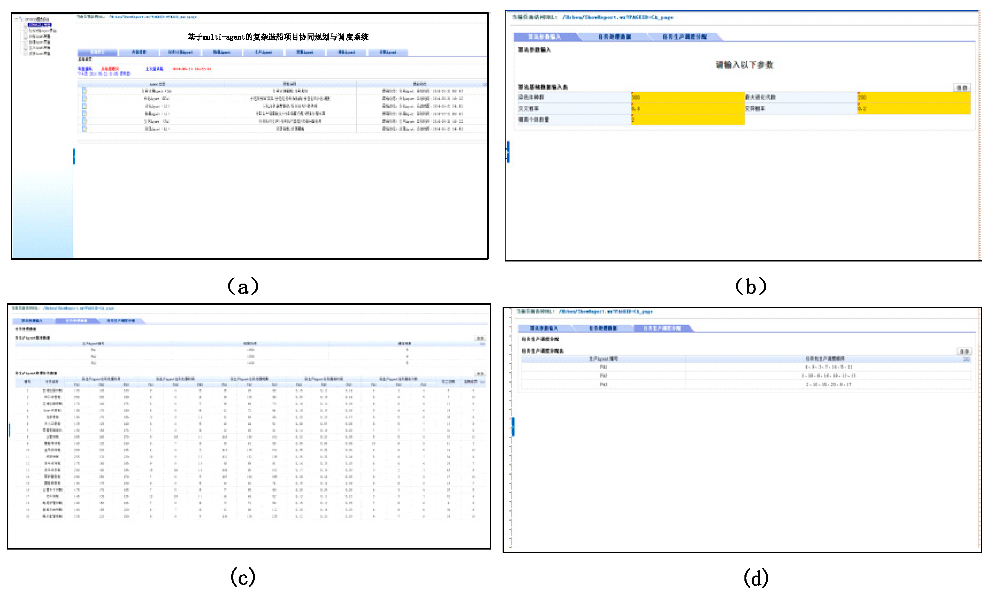
6. An Application Case

Java development language is used to develop the prototype system—Complex Shipbuilding Projects Collaborative Planning and Scheduling System (CSPCPSS) in the form of a Java Web project. The development technology framework adopts the lightweight spring framework, which focuses on solving the complexity of enterprise application development. The public infrastructure layer is combined with the object relational mapping framework Hibernate for rapid data operation. The foreground adopts the EASY-UI technology framework, and the database adopts the large relational database Oracle 11 G by invoking the JAR package in the Spring control layer (Controller) to realize complex business proxy functions. The screenshots of the key functional interfaces in the prototype system are made, as shown in Figure 13.

7. Conclusions

In this paper, an assistant decision-making method is provided to support effective task dispatching and multi-party cooperation for better utilization of the distributed resource, thus helping project managers control the shipbuilding process. The proposed method effectively solved a new complex problem in the shipbuilding background, including a multi-mode resource constraint multi-project scheduling problem under flexible task duration and distributed resource-constrained project planning problems. To articulate the problem, a complex shipbuilding project distributed cooperative planning and scheduling problem model is proposed, combining the project planning and scheduling process. As a matter of fact, in many similar large-scale projects, there is no connection between scheduling and planning problems, which leads to inaccurate scheduling schemes and more frequent changes. The research in this paper provides a reference: the distributed scheduling process can be effectively connected by parameterizing the local optimization and the interorganizational coordination process.

From the perspective of engineering applications, a multi-agent-based project planning and scheduling framework was proposed, which simulated the collaborative decision-making planning and symmetric scheduling process, filling the research gap. The designed framework includes two symmetrical modules, a planning module and a scheduling module, connecting the multi-project planning with a single project scheduling in detail, wherein a negotiation method is proposed to solve the integration problem of distributed local optimization and coordination between organizations. The experiments verify the effectiveness and rationality of the framework and method. From the academic perspective, this research contributes to the parallel planning problem solving for distributed large-scale complex engineering projects. Current and future work can be dedicated to expanding the system by designing more negotiation methods to deal with more possible engineering situations.

References

1. Zhang, A.N.; Ma, B.; Loke, D.; Kumar, S.; Chan, Y.Y. Multi-project planning and optimisation for shipyard operations. In Proceedings of the IEEE International Conference on Industrial Engineering and Engineering Management, Hong Kong, China, 10–13 December 2012. [Google Scholar]
2. Hossain, K.A.; Golam Zakaria, N.M. A Study on Global Shipbuilding Growth, Trend and Future Forecast. Procedia Eng. 2017, 194, 247–253. [Google Scholar] [CrossRef]
3. Han, D.; Yang, B.; Li, J.; Wang, J.; Sun, M.; Zhou, Q. A multi-agent-based system for two-stage scheduling problem of offshore project. Advances Mech. Eng. 2017, 9, 1–17. [Google Scholar] [CrossRef]
4. Lee, Y.H.; Kumara, S.R.T.; Chatterjee, K. Multi-agent based dynamic resource scheduling for distributed multiple projects using a market mechanism. J. Intell. Manuf. 2003, 14, 471–484. [Google Scholar] [CrossRef]
5. Li, J.; Li, L.; Yang, B.; Zhou, Q. Development of a Collaborative Scheduling System of Offshore Platform Project Based on Multiagent Technology. Advances Mech. Eng. 2014, 298149. [Google Scholar] [CrossRef]
6. Järvenpää, E.; Lanz, M.; Siltala, N. Formal Resource and Capability Models supporting Re-use of Manufacturing Resources. Procedia Eng. 2018, 19, 87–94. [Google Scholar]
7. Thomas, A.; Singh, G.; Krishnamoorthy, M.; Venkateswaran, J. Distributed optimisation method for multi-resource constrained scheduling in coal supply chains. Int. J. Prod. Res. 2013, 51, 2740–2759. [Google Scholar] [CrossRef]
8. Thomas, A.; Venkateswaran, J.; Singh, G.; Krishnamoorthy, M. A resource constrained scheduling problem with multiple independent producers and a single linking constraint: A coal supply chain example. Eur. J. Oper. Res. 2014, 236, 946–956. [Google Scholar] [CrossRef]
9. Singh, G.; Ernst, A.T. Resource constraint scheduling with a fractional shared resource. Oper. Res. Lett. 2011, 39, 363–368. [Google Scholar] [CrossRef]
10. Tavana, M.; Abtahi, A.R.; Damghani, K.K. A new multi-objective multi-mode model for solving preemptive time-cost-quality trade-off project scheduling problems. Expert Syst. Appl. 2014, 41, 1830–1846. [Google Scholar] [CrossRef]
11. Fu, N.; Lau, H.C.; Varakantham, P. Robust execution strategies for project scheduling with unreliable resources and stochastic durations. J. Sched. 2015, 18, 607–622. [Google Scholar] [CrossRef]
12. Rostami, S.; Creemers, S.; Leus, R. New strategies for stochastic resource-constrained project scheduling. J. Sched. 2018, 21, 349–365. [Google Scholar] [CrossRef]
13. Liu, C.; Xiang, X.; Zheng, L.; Ma, J. An integrated model for multi-resource constrained scheduling problem considering multi-product and resource-sharing. Int. J. Prod. Res. 2018, 56, 6491–6511. [Google Scholar] [CrossRef]
14. Lau, J.S.; Huang, G.Q.; Mak, K.L.; Liang, L. Agent-based modeling of supply chains for distributed scheduling. IEEE Trans. Syst. Man Cybern. A Syst. Hum. 2006, 36, 847–861. [Google Scholar] [CrossRef] [Green Version]
15. Confessore, G.; Giordani, S.; Rismondo, S. A market-based multi-agent system model for decentralized multi-project scheduling. Ann. Oper. Res. 2007, 150, 115–135. [Google Scholar] [CrossRef]
16. Homberger, J. A (μ, λ)-coordination mechanism for agent-based multi-project scheduling. OR Spectr. 2007, 34, 107–132. [Google Scholar] [CrossRef]
17. Adhau, S.; Mittal, M.L.; Mittal, A. A multi-agent system for decentralized multi-project scheduling with resource transfers. Int. J. Prod. Econ. 2013, 146, 646–661. [Google Scholar] [CrossRef]
18. Zheng, Z.; Guo, Z.; Zhu, Y.; Zhang, X. A critical chains based distributed multi-project scheduling approach. Neurocomputing 2014, 143, 282–293. [Google Scholar] [CrossRef]
19. Du, B.; Zhou, H. A robust optimization approach to the multiple allocation p-center facility location problem. Symmetry 2018, 10, 588. [Google Scholar] [CrossRef] [Green Version]
20. Liu, L.; Su, J.; Zhao, B.; Wang, Q.; Chen, J.; Luo, Y. Towards an efficient privacy-preserving decision tree evaluation service in the Internet of Things. Symmetry 2020, 12, 103. [Google Scholar] [CrossRef] [Green Version]
21. Zeng, S.; Hussain, A.; Mahmood, T.; Ali, M.I.; Ashraf, S.; Munir, M. Covering-based spherical fuzzy rough set model hybrid with TOPSIS for multi-attribute decision-making. Symmetry 2019, 11, 547. [Google Scholar] [CrossRef] [Green Version]
22. Kucharska, E. Dynamic vehicle routing problem predictive and unexpected customer availability. Symmetry 2019, 11, 546. [Google Scholar] [CrossRef] [Green Version]
23. Zavadskas, E.K.; Bausys, R.; Antucheviciene, J. Civil engineering and symmetry. Symmetry 2019, 11, 501. [Google Scholar] [CrossRef] [Green Version]
24. Jeong, H.; CHA, K. An ecient mapreduce-based parallel processing framework for user-based collaborative filtering. Symmetry 2019, 11, 748. [Google Scholar] [CrossRef] [Green Version]
25. Kim, B.; Byun, H.; Heo, Y.; Jeong, Y. Adaptive job load balancing scheme on mobile cloud computing with collaborative architecture. Symmetry 2017, 9, 65. [Google Scholar] [CrossRef]
26. Machuca, M.D.B.; Chinthammit, W.; Huang, W.; Wasinger, R.; Duh, H. Enabling symmetric collaboration in public spaces through 3D mobile interaction. Symmetry 2018, 10, 69. [Google Scholar] [CrossRef] [Green Version]
27. Wu, Y.; He, F.; Han, S. Collaborative CAD synchronization based on a symmetric and consistent modeling procedure. Symmetry 2017, 9, 59. [Google Scholar] [CrossRef] [Green Version]
28. Dursun, M.; Arslan, Ö. An integrated decision framework for material selection procedure: A case study in a detergent manufacturer. Symmetry 2018, 10, 657. [Google Scholar] [CrossRef] [Green Version]
29. Yang, W.; Hu, Y.; Hu, C.; Yang, M. An agent-based simulation of deep foundation pit emergency evacuation modeling in the presence of collapse disaster. Symmetry 2018, 10, 581. [Google Scholar] [CrossRef] [Green Version]
30. Wang, L.; Lin, S. A multi-agent based agile manufacturing planning and control system. Comput. Ind. Eng. 2009, 57, 620–640. [Google Scholar] [CrossRef]
31. Reddy, R.H.; Kumar, S.K.; Fernandes, K.J.; Tiwari, M.K. A Multi-Agent System based simulation approach for planning procurement operations and scheduling with multiple cross-docks. Comput. Ind. Eng. 2017, 107, 289–300. [Google Scholar] [CrossRef]
32. Lu, L.; Wang, G. A study on multi-agent supply chain framework based on network economy. Comput. Ind. Eng. 2008, 54, 288–300. [Google Scholar] [CrossRef]
33. Hsu, C.; Kao, B.; Ho, V.; Li, L.; Lai, K.R. An agent-based fuzzy constraint-directed negotiation model for solving supply chain planning and scheduling problems. Appl. Soft Comput. 2016, 48, 703–715. [Google Scholar] [CrossRef]
34. Yoon, D.Y.; Kim, G.C. A concept design for development of process planning and scheduling support system. Bull. Soc. Nav. Archit. Korea 1993, 30, 37–40. [Google Scholar]
35. Choi, H.R.; Ryu, K.R.; Cho, K.K.; Lim, H.S.; Hwan, J.H. A scheduling system for panel block assembly shop in shipbuilding using genetic algorithms. J. Intell. Inf. Syst. 1996, 2, 29–42. [Google Scholar]
36. Cho, K.K.; Kim, Y.G. An operation scheduling system for hull fabrication shop. In Proceedings of the Korean Operations and Management Science Society Conference, Pohang, Korea, 1 April 1997; pp. 443–446. [Google Scholar]
37. Woo, S.B.; Ryu, H.G.; Hahn, H.S. Heuristic algorithms for resource leveling in pre-erection scheduling and erection scheduling of shipbuilding. IE Interfaces 2003, 16, 332–343. [Google Scholar]
38. Persona, A.; Regattieri, A.; Romano, P. An integrated reference model for production planning and control in SMEs. J. Manuf. Technol. Manag. 2004, 15, 626–640. [Google Scholar] [CrossRef]
39. Liu, Z.; Chua, D.; Yeoh, K.W. Aggregate Production Planning for Shipbuilding with Variation-Inventory Trade-Offs. Int. J. Prod. Res. 2011, 49, 6249–6272. [Google Scholar] [CrossRef]
40. Kim, Y.S.; Lee, D.H. A Study on Construction of Detail Integrated Scheduling System of Ship Building Process. J. Soc. Nav. Archit. Korea 2007, 44, 48–54. [Google Scholar] [CrossRef] [Green Version]
41. Lee, D.H.; Kim, Y.S.; Kim, J.H. A study on real-time planning system in multi progress planning environment. J. Soc. Nav. Archit. Korea 2008, 45, 547–553. [Google Scholar] [CrossRef]
42. Dong, F.; Deglise-Hawkinson, J.R.; Van Oyen, M.P.; Singer, D.J. Dynamic control of a closed two-stage queueing network for outfitting process in shipbuilding. Comput. Oper. Res. 2016, 72, 1–11. [Google Scholar] [CrossRef] [Green Version]
43. Back, M.G.; Woo, J.H.; Lee, P.; Shin, J.G. Productivity improvement strategies using simulation in offshore plant construction. J. Ship Prod. Design 2017, 33, 144–155. [Google Scholar] [CrossRef]
44. Mello, M.H.; Gosling, J.; Naim, M.M.; Strandhagen, J.O.; Brett, P.O. Improving coordination in an engineer-to-order supply chain using a soft systems approach. Prod. Plan. Control 2017, 28, 89–107. [Google Scholar] [CrossRef]
45. Hartmann, S.; Briskorn, D. A survey of variants and extensions of the resource constrained project scheduling problem. Eur. J. Oper. Res. 2010, 207, 1–14. [Google Scholar] [CrossRef] [Green Version]
46. Weglarz, J.; Józefowska, J.; Mika, M.; Waligóra, G. Project scheduling with finite or infinite number of activity processing modes—A survey. Eur. J. Oper. Res. 2011, 208, 177–205. [Google Scholar] [CrossRef]
47. Tritschler, M.; Naber, A.; Kolisch, R. A hybrid metaheuristic for resource-constrained project scheduling with flexible resource profiles. Eur. J. Oper. Res. 2017, 262, 262–273. [Google Scholar] [CrossRef]
48. Hartmann, S. Project scheduling with multiple modes: A genetic algorithm. Ann. Oper. Res. 2001, 102, 111–135. [Google Scholar] [CrossRef]
49. Alcaraz, J.; Maroto, C.; Ruiz, R. Solving the multi-mode resource constrained project scheduling problem with genetic algorithms. J. Oper. Res. Soc. 2003, 54, 614–626. [Google Scholar] [CrossRef]
50. Koulinas, G.; Kotsikas, L.; Anagnostopoulos, K. A particle swarm optimization based hyper-heuristic algorithm for the classic resource constrained project scheduling problem. Inf. Sci. 2014, 277, 680–693. [Google Scholar] [CrossRef]
51. Bettemir, O.H.; Sonmez, R. Hybrid genetic algorithm with simulated annealing for resource-constrained project scheduling. J. Manag. Eng. 2014, 31, 04014082. [Google Scholar] [CrossRef]
52. Messelis, T.; Causmaecker, P.D. An automatic algorithm selection approach for the multi-mode resource-constrained project scheduling problem. Eur. J. Oper. Res. 2014, 233, 511–528. [Google Scholar] [CrossRef]
53. Zheng, X.L.; Wang, L. A multi-agent optimization algorithm for resource constrained project scheduling problem. Expert Syst. Appl. 2015, 42, 6039–6049. [Google Scholar] [CrossRef]
54. Sonmez, R.; Gurel, M. Hybrid optimization method for large-scale multimode resource-constrained project scheduling problem. J. Manag. Eng. 2016, 32, 04016020. [Google Scholar] [CrossRef]
55. Dong, Z.S.; Tao, S.; Shi, Q. Coupling resource allocation and project scheduling considering resource scarcity. In Proceeding of the 2018 IISE Annual Conference, Orlando, FL, USA, 19–22 May 2018; pp. 1801–1806. [Google Scholar]
56. Wang, L.; Zhan, D.; Nie, L.; Xu, X.; Zhang, Z. Optimization method for block erection scheduling with activity duration elasticity. Comput. Integr. Manuf. Syst. 2011, 17, 1478–1485. [Google Scholar]
57. Confessore, G.; Giordani, S.; Rismondo, S. An auction based approach in decentralized project scheduling. In Proceeding of the PMS 2002—International Workshop on Project Management and Scheduling, Valencia, Spain, 3–5 April 2002; pp. 110–113. [Google Scholar]
58. Lau, J.S.; Huang, G.Q.; Mak, K.L.; Liang, L. Distributed project scheduling with information sharing in supply chains: Part I—An agent-based negotiation model. Int. J. Prod. Res. 2005, 43, 4813–4838. [Google Scholar] [CrossRef]
59. Martins, P.J. Distributed production planning and control agent-based system. Int. J. Prod. Res. 2006, 44, 3693–3709. [Google Scholar]
60. Homberger, J. A multi-agent system for the decentralized resource constrained multi-project scheduling. Int. Trans. Oper. Res. 2007, 14, 565–589. [Google Scholar] [CrossRef]
61. Aysegul, T.; Ihsan, S. Distributed scheduling: A review of concepts and applications. Int. J. Prod. Res. 2010, 48, 5235–5262. [Google Scholar]
62. Cao, Y.; Yu, W.; Ren, W.; Chen, G. An overview of recent progress in the study of distributed multi-agent coordination. IEEE Trans. Ind. Inform. 2013, 9, 427–438. [Google Scholar] [CrossRef] [Green Version]
63. Behnamian, J.; Ghomi, S.M.F. A survey of multi-factory scheduling. J. Intell. Manuf. 2016, 27, 231–249. [Google Scholar] [CrossRef]
64. Ben-Zvi, T.; Lechler, T.G. Resource allocation in multi-project environments: Planning vs. execution strategies. Proc. PICMET 2011, 11, 1–7. [Google Scholar] [CrossRef]
65. Deb, K.; Pratap, A.; Agarwal, S.; Meyarivan, T.A.M.T. A fast and elitist multiobjective genetic algorithm: NSGA-II. IEEE Trans. Evol. Comput. 2002, 6, 182–197. [Google Scholar] [CrossRef] [Green Version]
66. Murugan, P.; Kannan, S.; Baskar, S. NSGA-II algorithm for multi-objective generation expansion planning problem. Electr. Power Syst. Res. 2009, 79, 622–628. [Google Scholar] [CrossRef]
67. Huang, B.; Buckley, B.; Kechadi, T.M. Multi-objective feature selection by using NSGA-II for customer churn prediction in telecommunications. Expert Syst. Appl. 2010, 37, 3638–3646. [Google Scholar] [CrossRef]
68. Jeyadevi, S.; Baskar, S.; Babulal, C.K.; Iruthayarajan, M.W. Solving multiobjective optimal reactive power dispatch using modified NSGA-II. Int. J. Electr. Power Energy Syst. 2011, 33, 219–228. [Google Scholar] [CrossRef]
69. Ramesh, S.; Kannan, S.; Baskar, S. Application of modified NSGA-II algorithm to multi-objective reactive power planning. Appl. Soft Comput. J. 2012, 12, 741–753. [Google Scholar] [CrossRef]
70. Xu, Z.; Ming, X.G.; Zheng, M.; Li, M.; He, L.; Song, W. Cross-trained workers scheduling for field service using improved NSGA-II. Int. J. Prod. Res. 2015, 53, 1255–1272. [Google Scholar] [CrossRef]
71. Zhong, W.; Liu, J.; Xue, M.; Jiao, L. A multiagent genetic algorithm for global numerical optimization. IEEE Trans. Syst. Man Cybern. B Cybern. 2004, 34, 1128–1141. [Google Scholar] [CrossRef]
72. Ghoddousi, P.; Eshtehardian, E.; Jooybanpour, S.; Javanmardi, A. Multi-mode resource-constrained discrete time-cost-resource optimization in project scheduling using non-dominated sorting genetic algorithm. Autom. Constr. 2013, 30, 216–227. [Google Scholar] [CrossRef]
73. Cao, D.; Murat, A.; Chinnam, R.B. Efficient exact optimization of multi-objective redundancy allocation problems in series-parallel systems. Reliab. Eng. Syst. Saf. 2013, 111, 154–163. [Google Scholar] [CrossRef]
74. Kuo, T. A modified topsis with a different ranking index. Eur. J. Oper. Res. 2017, 260, 152–160. [Google Scholar] [CrossRef]
75. Walczak, D.; Rutkowska, A. Project rankings for participatory budget based on the fuzzy TOPSIS method. Eur. J. Oper. Res. 2017, 260, 706–714. [Google Scholar] [CrossRef]
76. Chauhan, R.; Singh, T.; Tiwari, A.; Patnaik, A.; Thakur, N.S. Hybrid entropy-TOPSIS approach for energy performance prioritization in a rectangular channel employing impinging air jets. Energy 2017, 134, 360–368. [Google Scholar] [CrossRef]
77. Huang, W.; Shuai, B.; Wang, Y.; Antwi, E. Using entropy-TOPSIS method to evaluate urban rail transit system operation performance: The China case. Transp. Res. A 2018, 111, 292–303. [Google Scholar] [CrossRef]
Figure 1. Cross-enterprise cooperation in shipbuilding projects.
Symmetry 12 00161 g001
Figure 2. Complex shipbuilding planning and scheduling process.
Symmetry 12 00161 g002
Figure 3. The system framework.
Symmetry 12 00161 g003
Figure 4. The flowchart of the proposed algorithm.
Symmetry 12 00161 g004
Figure 5. The structure of the solution matrix.
Symmetry 12 00161 g005
Figure 6. Collaborative crossover operation.
Symmetry 12 00161 g006
Figure 7. Self-learning operation.
Symmetry 12 00161 g007
Figure 8. A scheduling Gantt chart of Project 1.
Symmetry 12 00161 g008
Figure 9. Resource request and conflicts after five iterations.
Symmetry 12 00161 g009
Figure 10. Resource request and conflicts after 10 iterations.
Symmetry 12 00161 g010
Figure 11. Resource request and conflicts after 15 iterations.
Symmetry 12 00161 g011
Figure 12. Resource request and conflicts after 18 iterations.
Symmetry 12 00161 g012
Figure 13. (a) System main interface; (b) Project scheduling agent work interface; (c) Summary list of resource requests; (d) Task assignment list.
Symmetry 12 00161 g013