Dynamical Properties of Dark Energy Models in Fractal Universe


Abstract
1. Introduction
2. Field Equations with Solutions
2.1. THDE
2.2. RHDE
2.3. SMHDE
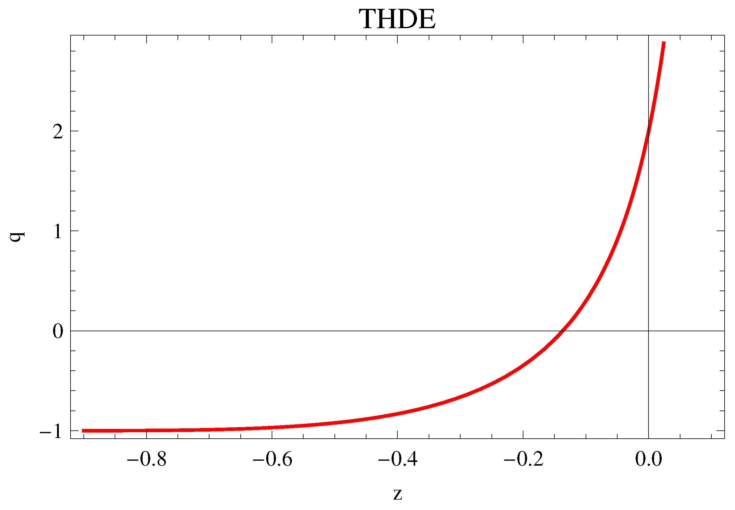
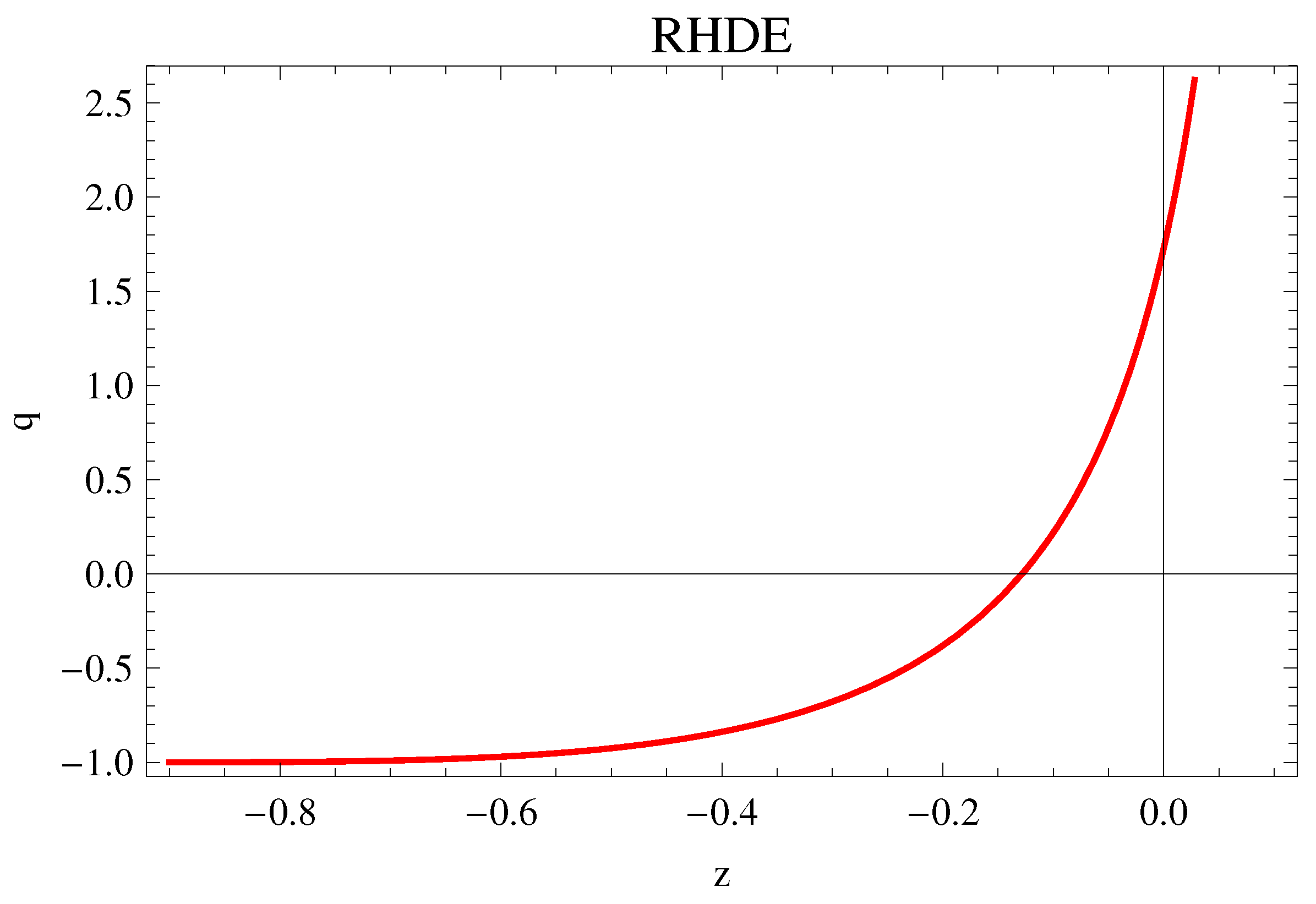
3. Deceleration Parameter
3.1. THDE
3.2. RHDE
3.3. SMHDE
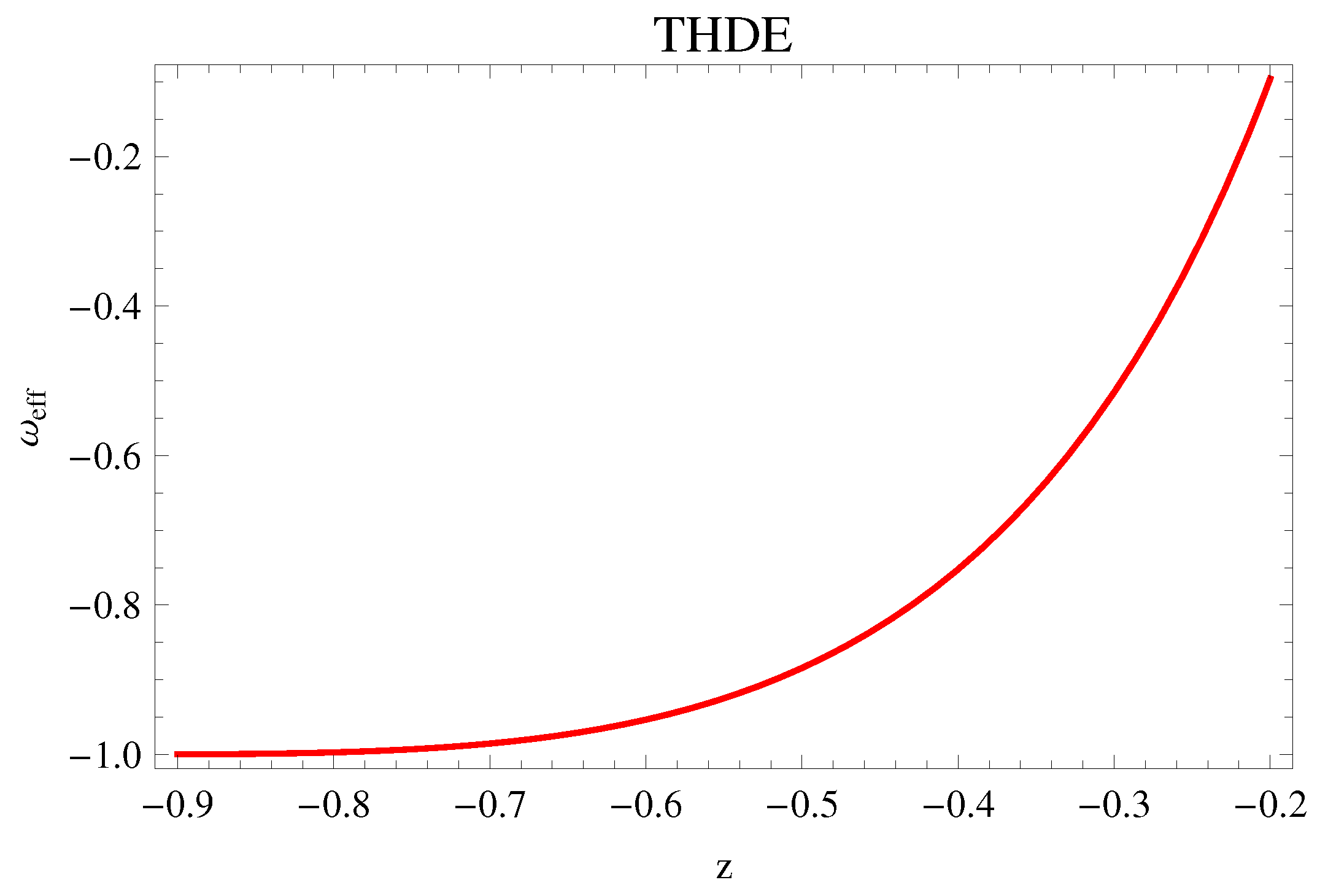
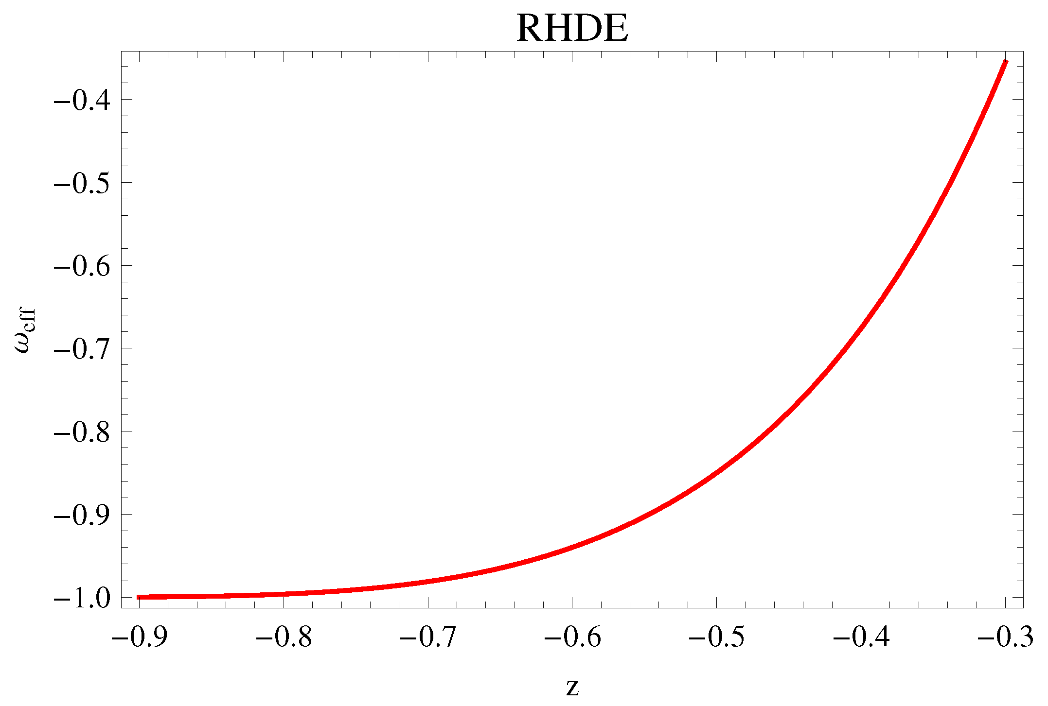
4. Eos Parameter
4.1. THDE
4.2. RHDE
4.3. SMHDE
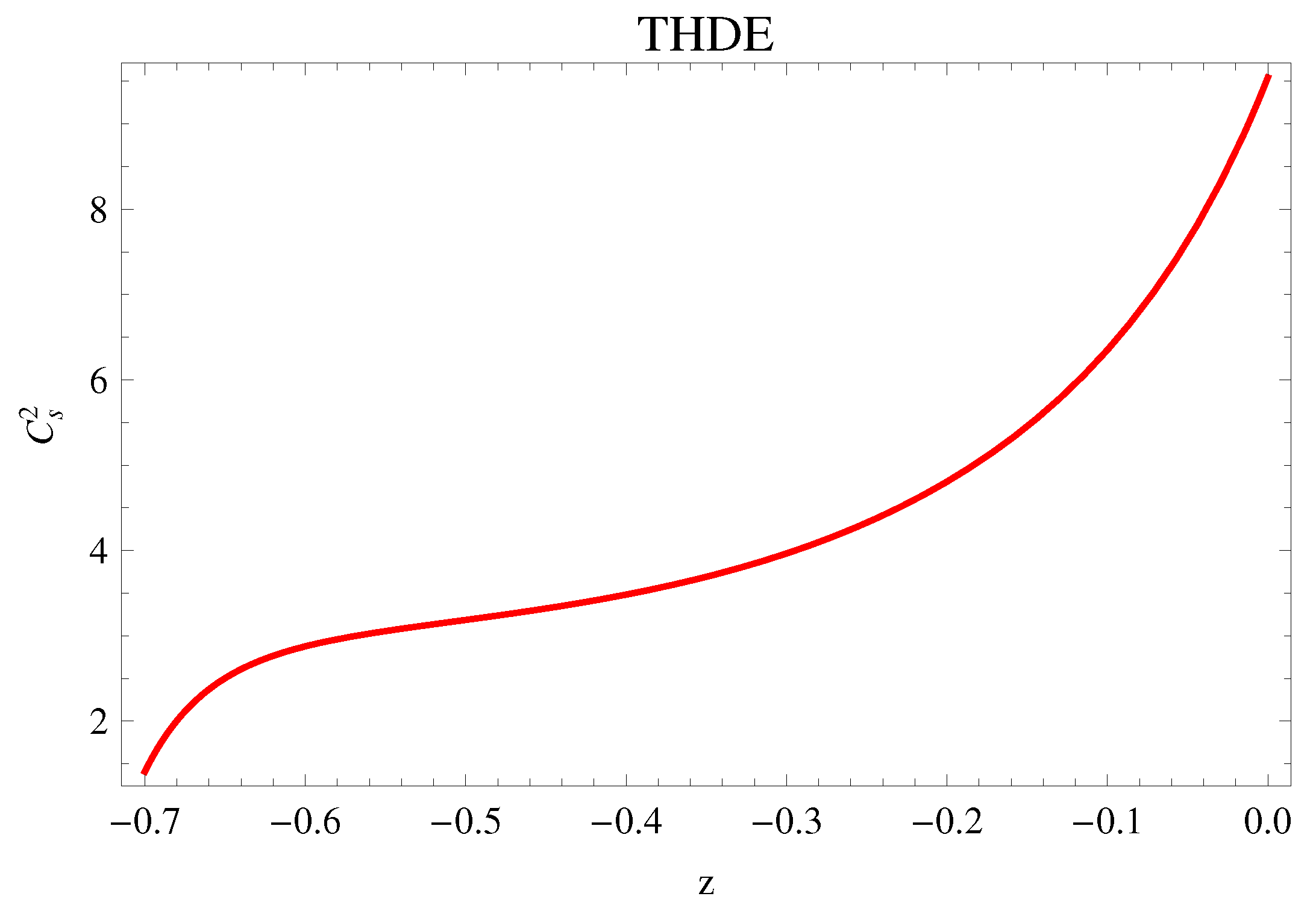
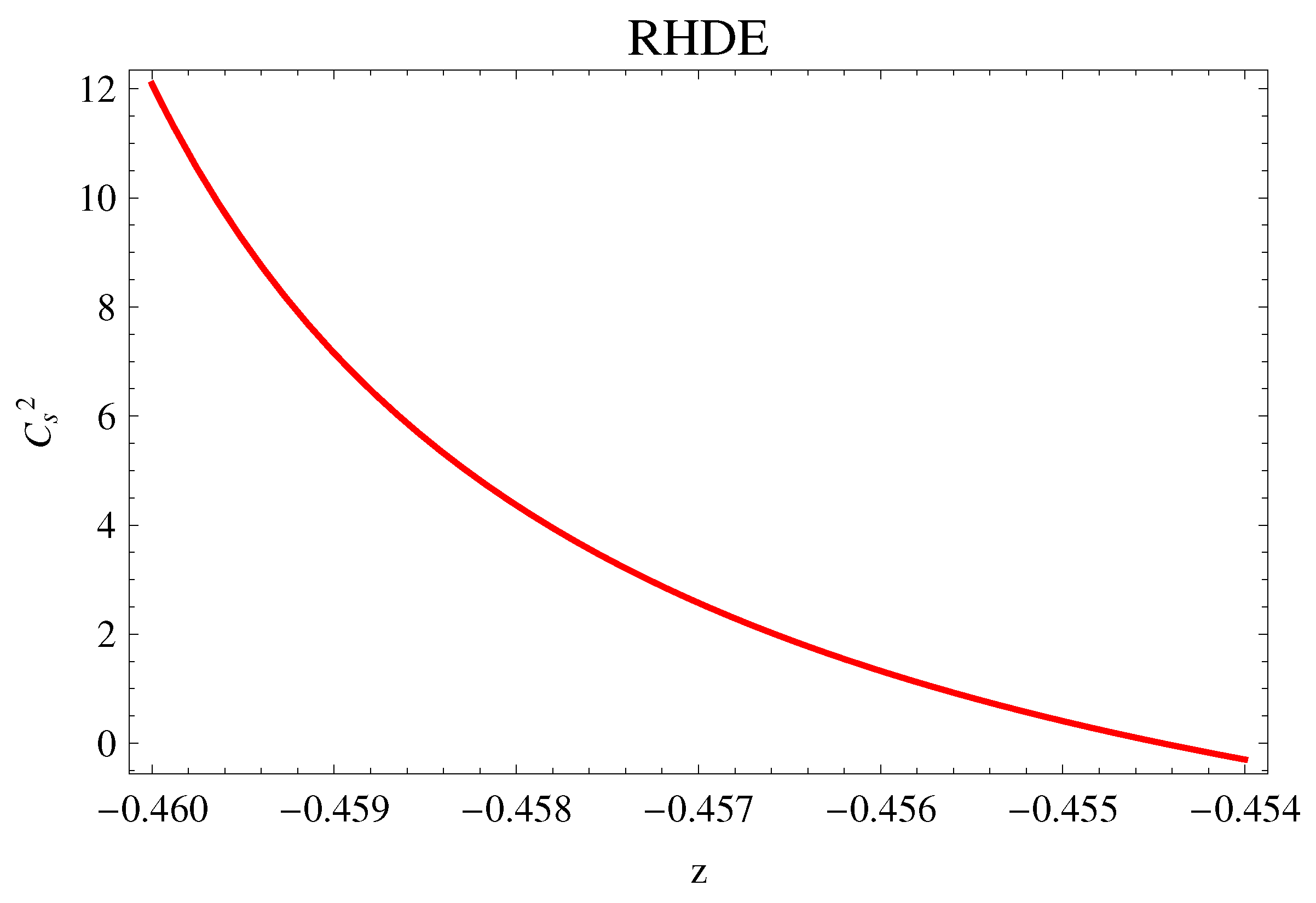
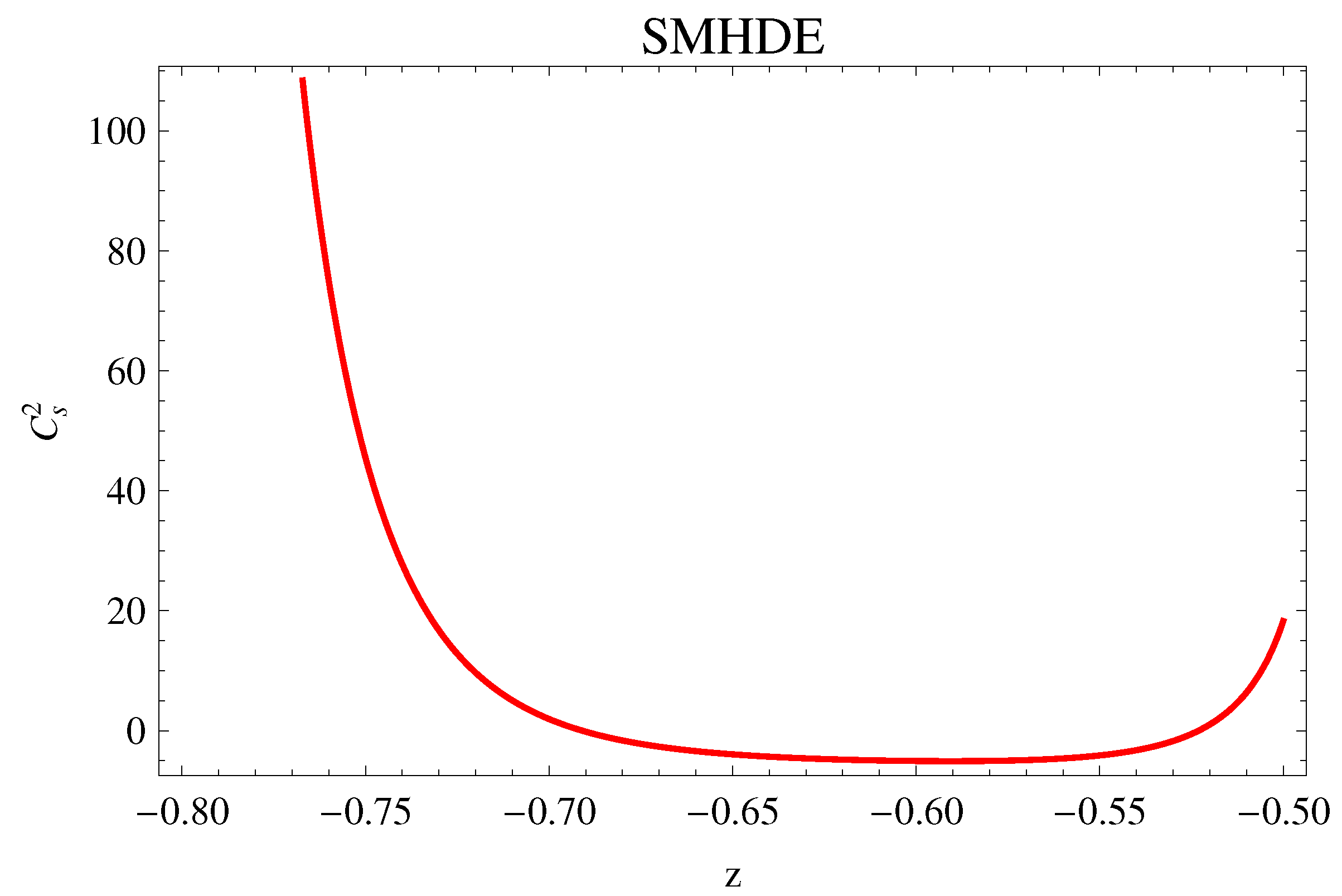
5. Square Speed Of Sound
5.1. THDE
5.2. RHDE
5.3. SMHDE
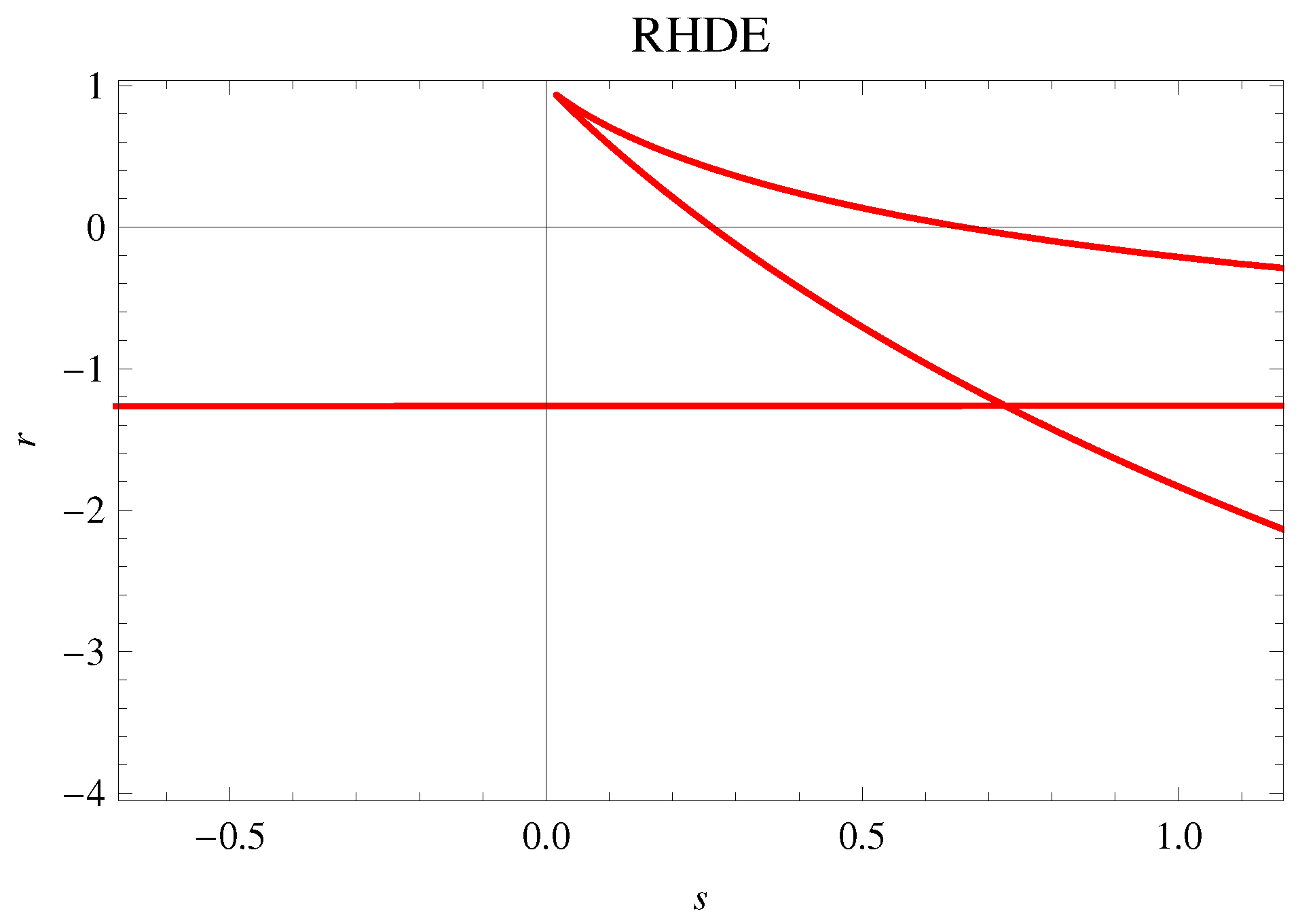
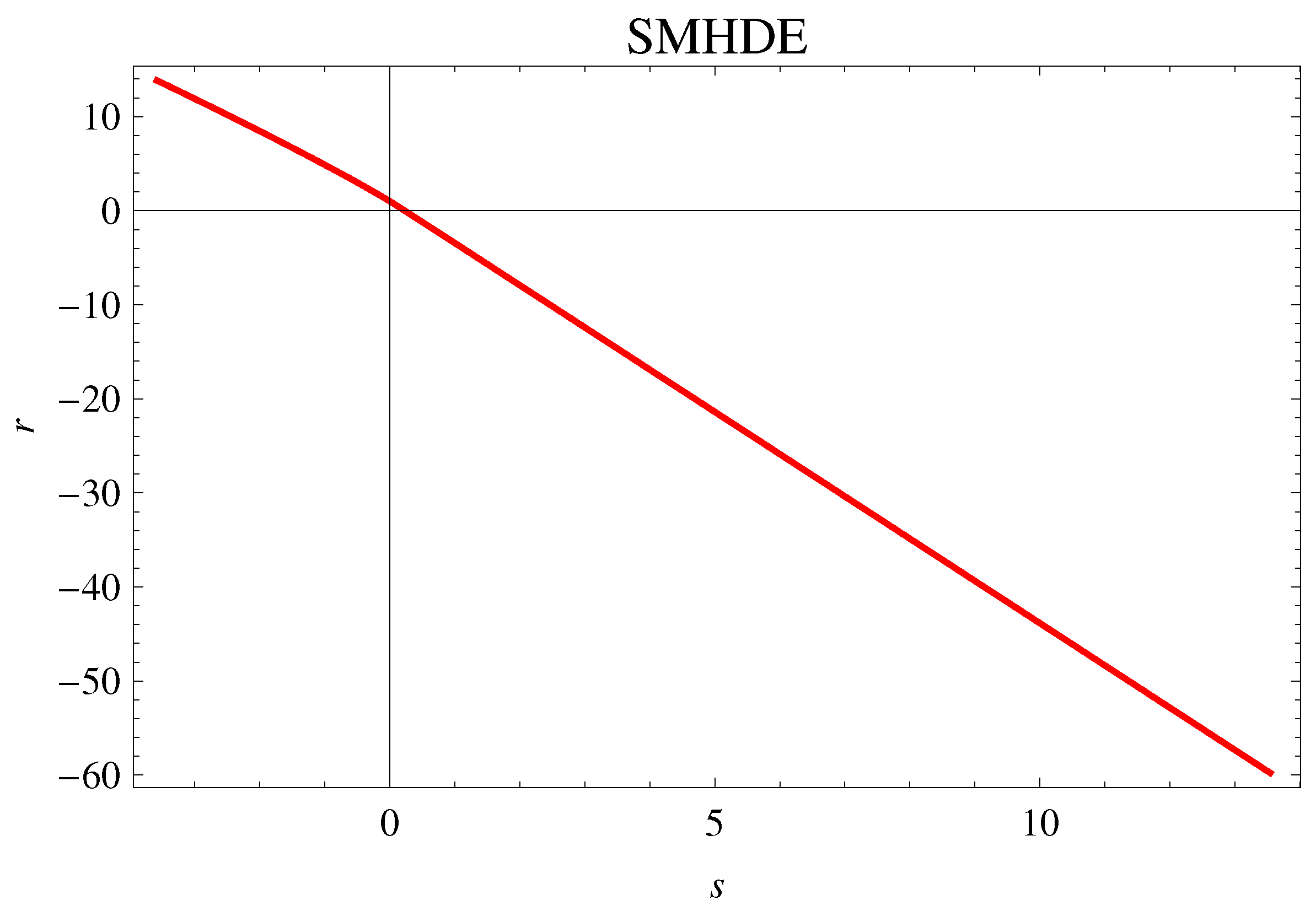
6. Statefinder Parameters
6.1. THDE
6.2. RHDE
6.3. SMHDE
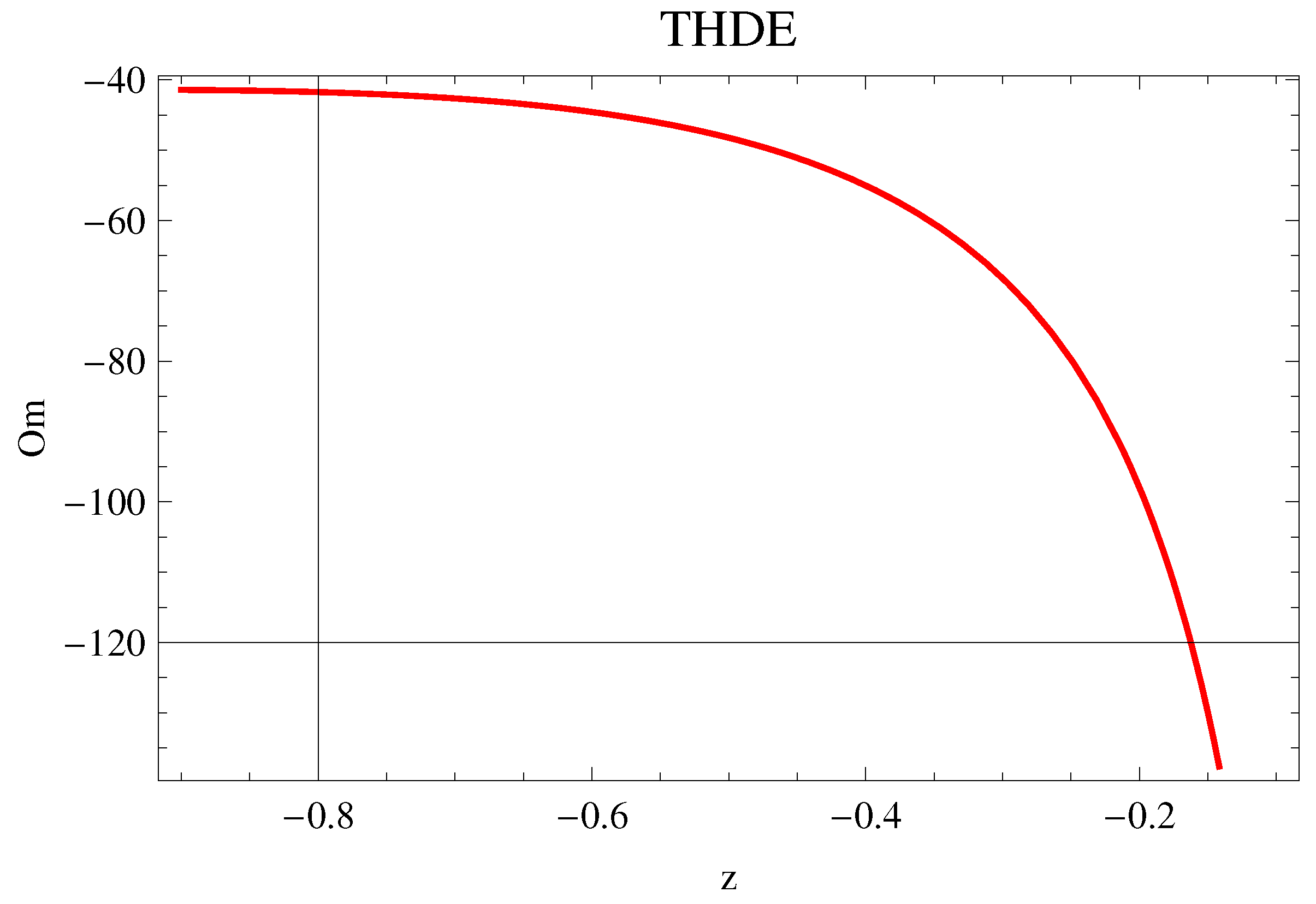
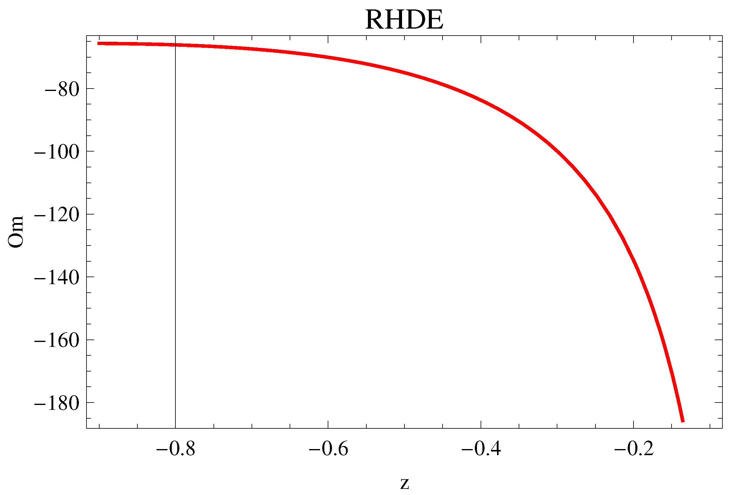
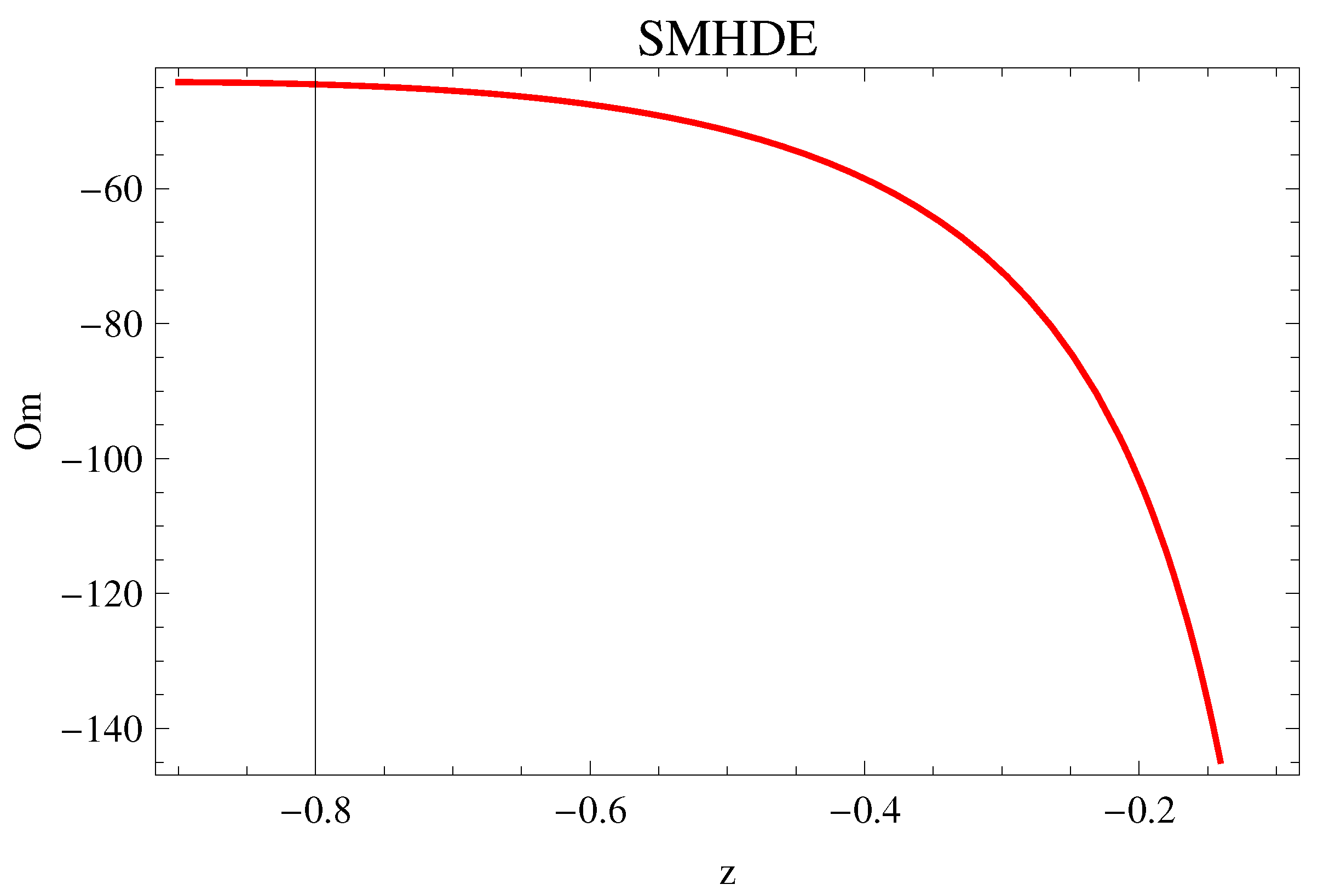
7. Om Parameter
8. - Plane Analysis
8.1. THDE
8.2. RHDE
8.3. SMHDE
9. Conclusions
Author Contributions
Funding
Acknowledgments
Conflicts of Interest
References
- Peebles, P.J.E. Principles of Physical Cosmology; Princeton University Press: Princeton, NJ, USA, 1993. [Google Scholar]
- Davis, M. Is the Universe Homogeneous on Large Scales? In Critical Dialogues in Cosmology; Turok, N., Ed.; World Scientific Publishing Company: Singapore, 1997; p. 13. [Google Scholar]
- Wu, K.K.S.; Lahav, O.; Rees, M. The Large-Scale Smoothness of the Universe. Nature 1999, 397, 225. [Google Scholar] [CrossRef]
- Joyce, M.; Montuori, M.; Sylos, L.F.; Pietronero, L. Comment on the paper “the eso slice project galaxy redshift survey: v. evidence for a d=3 sample dimensionality”. Astron. Astrophys. 1999, 344, 387. [Google Scholar]
- Coles, P. Cosmology: An unprincipled Universe? Nature 1998, 391, 120. [Google Scholar] [CrossRef]
- Smoot, G.; Bennett, C.L.; Kogut, A.; Wright, E.L.; Aymon, J.; Boggess, N.W.; Cheng, E.S.; de Amici, G.; Gulkis, S.; Hauser, M.G.; et al. Structure in the COBE differential microwave radiometer first-year maps. Astrophys. J. 1992, 396, L1. [Google Scholar] [CrossRef]
- Joyce, M.; Anderson, P.W.; Montuori, M.; Sylos Labini, F.; Pietronero, L. Fractal Cosmology in an Open Universe. Europhys. Lett. 2000, 49, 416. [Google Scholar] [CrossRef]
- Mandelbrot, B. The Fractal Geometry of Nature. Am. J. Phys. 1983, 51, 286. [Google Scholar] [CrossRef]
- Mandelbrot, B.B. Fractality, Lacunarity, and the Near-Isotropic Distribution of Galaxies. In Current Topics in Astrofundamental Physics: Primordial Cosmology; Sanchez, N., Zichichi, A., Eds.; NATO ASI Series (Series C: Mathematical and Physical Sciences); Springer: Dordrecht, The Netherlands, 1998; Volume 511, p. 583. [Google Scholar]
- Coleman, P.H.; Pietronero, L. The fractal structure of the universe. Phys. Rep. 1992, 213, 311. [Google Scholar] [CrossRef]
- Perlmutter, S.; Aldering, G.; Goldhaber, G.; Knop, R.A.; Nugent, P.; Castro, P.G.; Deustua, S.; Fabbro, S.; Goobar, A.; Groom, D.E.; et al. Measurements of Ω and Λ from 42 high-redshift supernovae. Astrophys. J. 1999, 517, 565. [Google Scholar] [CrossRef]
- Abazajian, K.; Adelman-McCarthy, J.K.; Agüeros, M.A.; Allam, S.S.; Anderson, K.S.; Anderson, S.F.; Annis, J.; Bahcall, N.A.; Baldry, I.K.; Bastian, S.; et al. The second data release of the sloan digital sky survey. Astron. J. 2004, 128, 502. [Google Scholar] [CrossRef]
- Riess, A.G.; Filippenko, A.V.; Challis, P.; Clocchiatti, A.; Diercks, A.; Garnavich, P.M.; Gilliland, R.L.; Hogan, C.J.; Jha, S.; Kirshner, R.P.; et al. Observational evidence from supernovae for an accelerating universe and a cosmological constant. Astron. J. 1998, 116, 1009. [Google Scholar] [CrossRef]
- Bamba, K.; Capozziello, S.; Nojiri, S.; Odintsov, S.D. Dark energy cosmology: the equivalent description via different theoretical models and cosmography tests. Astro. Phys. Space Sci. 2012, 342, 155–228. [Google Scholar] [CrossRef]
- Hooft, G. Dimensional Reduction in Quantum Gravity. arXiv 2009, arXiv:gr-qc/9310026v2. [Google Scholar]
- Susskind, L. The World as a Hologram. J. Math. Phys. 1995, 36, 6377. [Google Scholar] [CrossRef]
- Cohen, A.; Kaplan, D.; Nelson, A. Effective Field Theory, Black Holes, and the Cosmological Constant. Phys. Rev. Lett. 1999, 82, 4971. [Google Scholar] [CrossRef]
- Li, M. A Model of Holographic Dark Energy. Phys. Lett. B 2004, 603, 1. [Google Scholar] [CrossRef]
- Fischler, W.; Susskind, L. Holography and Cosmology. arXiv 1998, arXiv:hep-th/9806039. [Google Scholar]
- Nojiri, S.; Odintsov, S.D. Unifying phantom inflation with late-time acceleration: Scalar phantom non-phantom transition model and generalized holographic dark energy. Gen. Relativ. Gravit. 2006, 38, 1285–1304. [Google Scholar] [CrossRef]
- Nojiri, S.; Odintsov, S.D. Inhomogeneous equation of state of the universe: Phantom era, future singularity, and crossing the phantom barrier. Phys. Rev. D 2005, 72, 023003. [Google Scholar] [CrossRef]
- Sheykhi, A. Holographic scalar field models of dark energy. Phys. Rev. D 2011, 84, 107302. [Google Scholar] [CrossRef]
- Hu, B.; Ling, Y. Interacting dark energy, holographic principle, and coincidence problem. Phys. Rev. D 2006, 73, 123510. [Google Scholar] [CrossRef]
- Ma, Y.Z.; Gong, Y.; Chen, X. Features of holographic dark energy under combined cosmological constraints. Eur. Phys. J. C 2009, 60, 303. [Google Scholar] [CrossRef]
- Masi, M. A step beyond Tsallis and Renyi entropies. Phys. Lett. A 2005, 338, 217. [Google Scholar] [CrossRef]
- Tsallis, C. The Nonadditive Entropy Sq and Its Applications in Physics and Elsewhere: Some Remarks. Entropy 2011, 13, 1765. [Google Scholar] [CrossRef]
- Renyi, A. Probability Theory; North-Holland: Amsterdam, The Netherlands, 1970. [Google Scholar]
- Tsallis, C. Possible generalization of Boltzmann-Gibbs statistics. J. Stat. Phys. 1988, 52, 479. [Google Scholar] [CrossRef]
- Jahromi, A.S.; Moosavi, S.A.; Moradpour, H.; Graça, J.M.; Lobo, I.P.; Salako, I.G.; Jawad, A. Generalized entropy formalism and a new holographic dark energy model. J. Phys. Lett. B. 2018, 2, 52. [Google Scholar]
- Nojiri, S.; Odintsov, S.D.; Saridakis, E.N. Modified cosmology from extended entropy with varying exponent. Eur. Phys. J. C 2019, 79, 242. [Google Scholar] [CrossRef]
- Calcagni, G. Quantum field theory, gravity and cosmology in a fractal universe. JHEP 2010, 1003, 120. [Google Scholar] [CrossRef]
- Calcagni, G. Fractal universe and quantum gravity. Phys. Rev. Lett. 2010, 104, 251301. [Google Scholar] [CrossRef]
- Calcagni, G. Multi-scale gravity and cosmology. JCAP 2013, 12, 41. [Google Scholar] [CrossRef]
- Salvatelli, V.; Said, N.; Bruni, M.; Melchiorri, A.; Wands, D. Indications of a Late-Time Interaction in the Dark Sector. Phys. Rev. Lett. 2014, 113, 181301. [Google Scholar] [CrossRef]
- Yang, T.; Guo, Z.K. Reconstructing the interaction between dark energy and dark matter using Gaussian processes. Phys. Rev. D 2015, 91, 123533. [Google Scholar] [CrossRef]
- Feng, C.; Wang, B.; Su, R.-K. Testing the viability of the interacting holographic dark energy model by using combined observational constraints. JCAP 2007, 9, 005. [Google Scholar] [CrossRef]
- Zimdahl, W.; Pavon, D.; Chimento, L.P. Interacting Quintessence. Phys. Lett. B 2001, 521, 133. [Google Scholar] [CrossRef]
- Wang, B.; Zang, J.; Lin, C.-Y.; Abdalla, E.; Micheletti, S. Interacting dark energy and dark matter: Observational constraints from cosmological parameters. Nucl. Phys. B 2007, 778, 69–84. [Google Scholar] [CrossRef]
- Amendola, L.; Tsujikawa, S.; Sami, M. Phantom damping of matter perturbations. Phys. Lett. B 2006, 632, 155–158. [Google Scholar] [CrossRef]
- Ferreira, E.G.M.; Quintin, J.; Costa, A.A.; Abdalla, E.; Wang, B. Evidence for interacting dark energy from BOSS. arXiv 2017, arXiv:1412.2777. [Google Scholar] [CrossRef]
- Gupta, G.; Saridakis, E.N.; Sen, A.A. Nonminimal quintessence and phantom with nearly flat potentials. Phys. Rev. D 2009, 79, 123013. [Google Scholar] [CrossRef]
- Santos, L. Constraining interacting dark energy with CMB and BAO future surveys. Phys. Rev. D 2017, 96, 103529. [Google Scholar] [CrossRef]
- Tsallis, C.; Cirto, L.J.L. Black hole thermodynamical entropy. Eur. Phys. J. C 2013, 73, 2487. [Google Scholar] [CrossRef]
- Tavayef, M.; Sheykhi, A.; Bamba, K.; Moradpour, H. Tsallis Holographic Dark Energy. arXiv 2018, arXiv:1804.02983v1. [Google Scholar] [CrossRef]
- Majhi, A. Non-extensive Statistical Mechanics and Black Hole Entropy From Quantum Geometry. Phys. Lett. B 2017, 775, 32–36. [Google Scholar] [CrossRef]
- Komatsu, N. Cosmological model from the holographic equipartition law with a modified Rényi entropy. Eur. Phys. J. C 2017, 77, 229. [Google Scholar] [CrossRef]
- Moradpour, H.; Bonilla, A.; Abreu, E.M.C.; Neto, J.A. Accelerated cosmos in a nonextensive setup. Phys. Rev. D 2017, 96, 123504. [Google Scholar] [CrossRef]
- Czinner, V.G.; Iguchi, H. Black hole entropy and the zeroth law of thermodynamics. Int. J. Mod. Phys. D 2015, 24, 1542015. [Google Scholar] [CrossRef]
- Sharma, B.D.; Mitta, P. New nonadditive measures of entropy for discrete probability distributions. J. Math. Sci. 1975, 10, 28–40. [Google Scholar]
- Sharma, B.D.; Mitta, P. New non-additive measures of relative information. J. Cmbin Inform. Syst. Sci. 1977, 2, 122–132. [Google Scholar]
- Sahni, V. Statefinder—A new geometrical diagnostic of dark energy. JETP Lett. 2003, 77, 201–206. [Google Scholar] [CrossRef]
- Caldwell, R.R.; Linder, E.V. The Limits of Quintessence. Phys. Rev. Lett. 2005, 95, 141301. [Google Scholar] [CrossRef]
- Aviles, A.; Gruber, C.; Luongo, O.; Quevedo, H. Cosmography and constraints on the equation of state of the Universe in various parametrizations. Phys. Rev. D 2012, 86, 123516. [Google Scholar] [CrossRef]
- Ade, P.A.R. Planck 2015 results. XIII. Cosmological parameters. A&A 2016, 594, A13. [Google Scholar]
- Hinshaw, G.; Larson, D.; Komatsu, E.; Spergel, D.N.; Bennett, C.L.; Dunkley, J.; Nolta, M.R.; Halpern, M.; Hill, R.S.; Odegard, N.; et al. Nine-year Wilkinson Microwave Anisotropy Probe (WMAP) Observations: Cosmological Parameter Results. Astrophys. J. Suppl. 2013, 208, 19. [Google Scholar] [CrossRef]


© 2019 by the authors. Licensee MDPI, Basel, Switzerland. This article is an open access article distributed under the terms and conditions of the Creative Commons Attribution (CC BY) license (http://creativecommons.org/licenses/by/4.0/).
Share and Cite
Shahzad, M.U.; Iqbal, A.; Jawad, A. Dynamical Properties of Dark Energy Models in Fractal Universe. Symmetry 2019, 11, 1174. https://doi.org/10.3390/sym11091174
Shahzad MU, Iqbal A, Jawad A. Dynamical Properties of Dark Energy Models in Fractal Universe. Symmetry. 2019; 11(9):1174. https://doi.org/10.3390/sym11091174
Chicago/Turabian StyleShahzad, Muhammad Umair, Ayesha Iqbal, and Abdul Jawad. 2019. "Dynamical Properties of Dark Energy Models in Fractal Universe" Symmetry 11, no. 9: 1174. https://doi.org/10.3390/sym11091174
APA StyleShahzad, M. U., Iqbal, A., & Jawad, A. (2019). Dynamical Properties of Dark Energy Models in Fractal Universe. Symmetry, 11(9), 1174. https://doi.org/10.3390/sym11091174