Article

A Confront between Amati and Combo Correlations at Intermediate and Early Redshifts

1
Istituto Nazionale di Fisica Nucleare, Laboratori Nazionali di Frascati, 00044 Frascati, Italy
2
NNLOT, Al-Farabi Kazakh National University, Al-Farabi av. 71, 050040 Almaty, Kazakhstan
Symmetry 2020, 12(7), 1118; https://doi.org/10.3390/sym12071118
Submission received: 2 May 2020 / Revised: 5 June 2020 / Accepted: 3 July 2020 / Published: 5 July 2020
(This article belongs to the Special Issue Beyond the Standard Cosmological Model in the Multi-messenger Era)

Abstract

:
I consider two gamma-ray burst (GRB) correlations: Amati and Combo. After calibrating them in a cosmology-independent way by employing Beziér polynomials to approximate the Observational Hubble Dataset (OHD), I perform Markov Chain Monte Carlo (MCMC) simulations within the Λ CDM and the wCDM models. The results from the Amati GRB dataset do not agree with the standard Λ CDM model at a confidence level 3 σ . For the Combo correlation, all MCMC simulations give best-fit parameters which are consistent within 1– σ with the Λ CDM model. Pending the clarification of whether the diversity of these results is statistical, due to the difference in the dataset sizes, or astrophysical, implying the search for the most suited correlation for cosmological analyses, future investigations require larger datasets to increase the predictive power of both correlations and enable more refined analyses on the possible non-zero curvature of the Universe and the dark energy equation of state and evolution.

1. Introduction

As of today, type Ia supernovae (SNe Ia) are considered to be standard candles for high-precision distance determinations [1,2,3,4]. However, some flaws in the use of SNe Ia have been recently exposed. The first one consists of a possible luminosity evolution with the environments of SNe Ia, which plays a major role in the systematic uncertainties in their distance determination [5]. The second one is that SNe Ia are detectable at most at redshifts z≃2 [6] and, thus, they cannot be used alone to clear the degeneracy between the standard Λ CDM cosmological model and alternative dark energy (DE) scenarios [7,8,9,10].
To overcome the above second shortcoming, distance indicators covering a wide range of z have become essential for cosmological tests. In this respect, gamma-ray bursts (GRBs) have the advantage to be detectable up to z = 9.4 [11,12,13,14], with a peak in their redshift distribution at z∼2– 2.5 [15]. Despite being affected by selection and instrumental effects [16,17,18,19,20], in The last two decades, various phenomenological correlations between GRB photometric and spectroscopic properties have been proposed to convert GRBs into cosmic rulers [19,20,21,22,23,24,25,26,27,28,29,30]. However, the major effect jeopardizing the standardization of GRBs is the circularity problem, which is a consequence of the fact that, due to the lack of very low-redshift GRBs, energy-spectrum correlations have to be calibrated by assuming an a priori background cosmology and fitting procedures inevitably return an overall agreement with it [31].
Recently, a model-independent calibration conceived to overcome the circularity problem [32] has been applied to the most investigated correlation involving prompt emission rest-frame peak energy E p of the GRB ν F ν spectrum and the bolometric isotropic radiated energy E iso , the E p E iso correlation or Amati relation [19,20,21,23,33]. This calibration method utilizes the Observational Hubble Data (OHD) obtained from the differential age method applied to pairs of nearby galaxies [34,35] and provides, through a model-independent fitting, measurements of the Hubble rate H ( z ) at arbitrary redshifts without assuming an a priori cosmological model [32,36].
In this paper I perform cosmological fits on the distance moduli obtained from the calibration of the E p E iso correlation by means of a Markov Chain Monte Carlo (MCMC) technique by fixing the Hubble constant to the value obtained from the OHD calibration H 0 = ( 67.76 ± 3.68 ) km s 1 Mpc 1 [32]. I compare the standard Λ CDM paradigm with its simplest DE extension, i.e., The wCDM model. In doing so, I here include the data from the most recent SNe Ia dataset, i.e., The Pantheon sample [37], instead of the JLA sample [38] used in a previous work [32]. I also extend this analysis focusing on another GRB correlation named Combo [29], which relates E p with X-ray afterglow observables (such as the plateau luminosity L 0 in the rest-frame band 0.3 –10 keV and its rest-frame duration τ , and The late power-law decay index α ). Although for this correlation an alternative calibration has been proposed [29], I here apply the above one based on OHD [32] and perform cosmological fits on the distance moduli obtained from the Combo correlation by comparing, again, the Λ CDM and the wCDM models. Thence, the aim of this paper is to confront the results from the above cosmological fits from the Amati and Combo correlations.
In Section 2, I summarize the model-independent calibration method based on the use of OHD dataset [32]. In Section 3, I apply the above calibration technique to Amati and Combo correlations and obtain the corresponding GRB distance moduli μ A and μ C , respectively. In Section 4 I perform cosmological fits to get constraints on the cosmological parameters. In particular, in Section 4.1, I show how to employ the calibrated GRB correlations and fit a) GRB data alone and b) GRB data together with Pantheon SN Ia dataset [37] to get constraints on the matter parameter Ω m within the Λ CDM model. In Section 4.2, to obtain robust bounds on the DE parameter w within the wCDM model, I perform a fit by using only GRB+SN dataset. In Section 4.3, I summarize the results of the MCMC simulations from the above cosmological models. In Section 5, I discuss the results, draw conclusions, and identify the perspectives of this work.

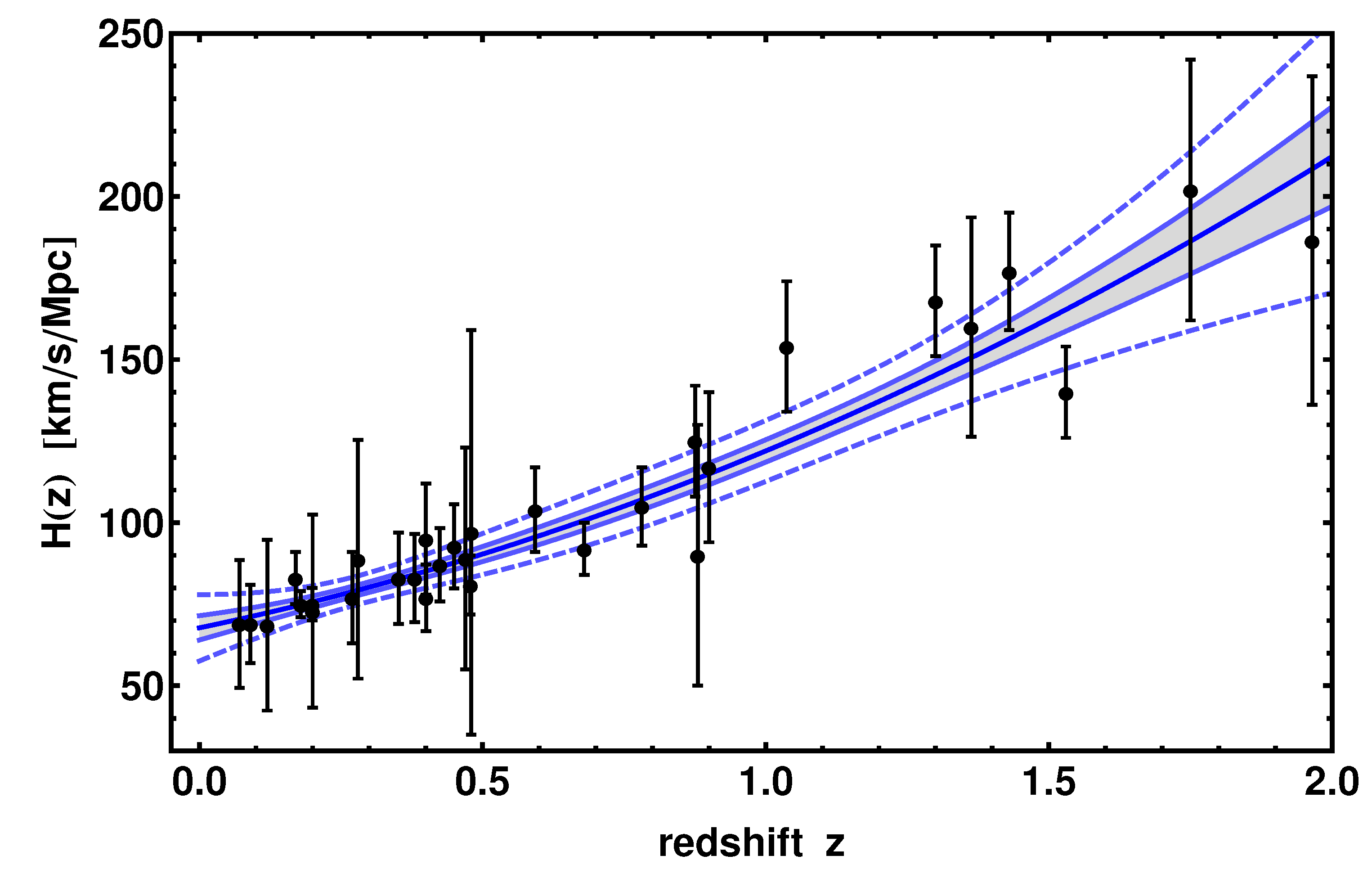
2. The OHD Model-Independent Calibration Method

The circularity problem affecting GRB correlations [17,19,22,31] enters in the definition of the generic energy/luminosity X through the luminosity distance d L , i.e., X z , H 0 , Ω i 4 π d L 2 z , H 0 , Ω i Y bolo , where Ω i are the cosmological parameters, and Y bolo is the rest-frame bolometric GRB fluence S bolo ( 1 + z ) 1 for the E iso definition, or The bolometric observed flux F bolo for the isotropic luminosity definitions. The use of any luminosity distance definition coming from other cosmological probes may bias the GRB Hubble diagram by introducing the systematics of the selected probe itself [20,30,31,39].
Thus, the need of model-independent techiques is essential to overcome the above issues [35,40,41,42,43,44,45,46,47,48,49,50,50]. However, the model is plagued by the convergence problem [51]. Thus, I introduce a new technique described in terms of polynomials and based directly on catalogs of data. In particular, I consider the OHD datapoints. These are cosmology-independent estimates of the Hubble function H ( z ) = ( 1 + z ) 1 Δ z / Δ t based on spectroscopic measurements of differential age Δ t and redshift difference Δ z [34]. The updated OHDs [35], shown in Figure 1, can be approximated by employing a Bézier parametric curve of degree n
H n ( x ) = d = 0 n β d h n d ( x ) , h n d ( x ) n ! x d 1 x n d d ! ( n d ) ! ,
where β d are coefficients of the linear combination of Bernstein basis polynomials h n d ( x ) , positive in the range 0 x z / z m 1 , where z max is the maximum z of the OHD. The only non-linear monotonic growing function up to z m is H 2 ( z ) obtained for n = 2 [32].
By using the above OHD interpolating function H 2 ( z ) , the luminosity distance writes as
d L ( Ω k , z ) = c H 0 ( 1 + z ) | Ω k | F k 0 z H 0 | Ω k | d z H 2 z ,
where F k ( x ) = sinh ( x ) for Ω k > 0 , F k ( x ) = x for Ω k = 0 , and F k ( x ) = sin ( x ) for Ω k < 0 . Imposing a curvature parameter Ω k = 0 , supported by Planck results [52], the luminosity distance becomes completly cosmology-independent
d cal ( z ) = c ( 1 + z ) 0 z d z H 2 ( z ) ,
enabling the calibration of the energy/luminosity
X cal ( z ) 4 π d cal 2 ( z ) Y bolo ,
where the errors σ X cal depend upon the GRB systematics and the statistical errors of the proposed correlation.

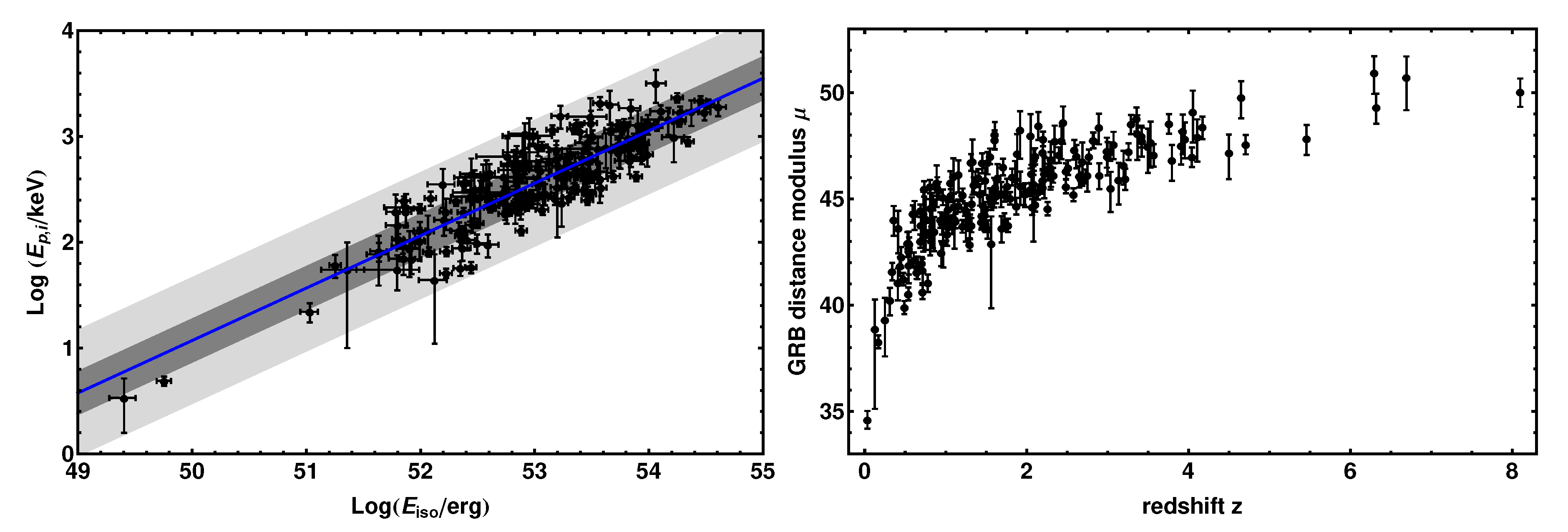
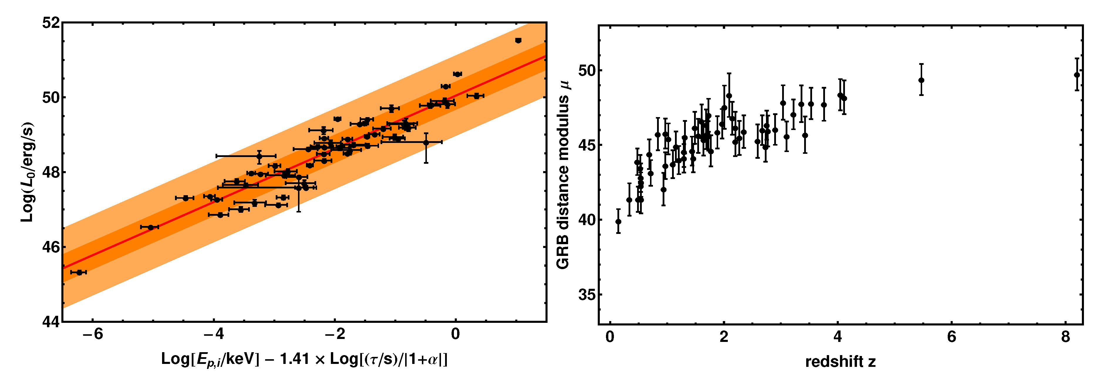
3. The Calibrated Amati and Combo Correlations

The E p E iso correlation is given by
log E p keV = q + m log E iso erg 52 .
By applying the procedure outlined in Section 2, from Equation (4) the calibrated isotropic energy writes as
E iso ( z ) 4 π d cal 2 ( z ) S bolo ( 1 + z ) 1 .
The fit of the calibrated correlation gives as best-fit parameters q = 2.06 ± 0.03 , m = 0.50 ± 0.02 , and The extra-scatter σ A = 0.20 ± 0.01 dex [32] (see Figure 2, left panel).
The 193 GRB distance moduli from the calibrated Amati correlation can be computed from the standard definition μ A = 25 + 5 log ( d cal / Mpc ) . In The specific case:
μ A = 32.55 + 5 2 1 m log E p keV q m log 4 π S bolo erg / c m 2 + log 1 + z .
The Hubble diagram of μ A with z and the corresponding attached errors, accounting for the GRB systematics and the statistical errors on q, m and σ A , are shown in Figure 2 (right panel).
The Combo correlation writes as [29]
log L 0 erg / s = a + b log E p keV log τ / s | 1 + α | ,
The calibration method in Equation (4) is here applied to the plateau luminosity L 0 as follows
L 0 ( z ) 4 π d cal 2 ( z ) F 0 ,
where F 0 is the rest-frame 0.3 –10 keV energy flux. The calibrated Combo correlation is shown in Figure 3 (left panel). Its best-fit parameters are a = 50.04 ± 0.27 , b = 0.71 ± 0.11 , and an extra-scatter σ C = 0.35 ± 0.04 .
The Hubble diagram of the 60 GRB distance moduli μ C and their attached errors accounting for the systematics and the statistical errors on a, b and σ C , obtained from the calibrated Combo correlation, are given by [29],
μ C = 97.45 + 5 2 log a erg / s + b log E p keV log τ / s | 1 + α | log 4 π F 0 erg / c m 2 / s
and are shown in Figure 3 (right panel).

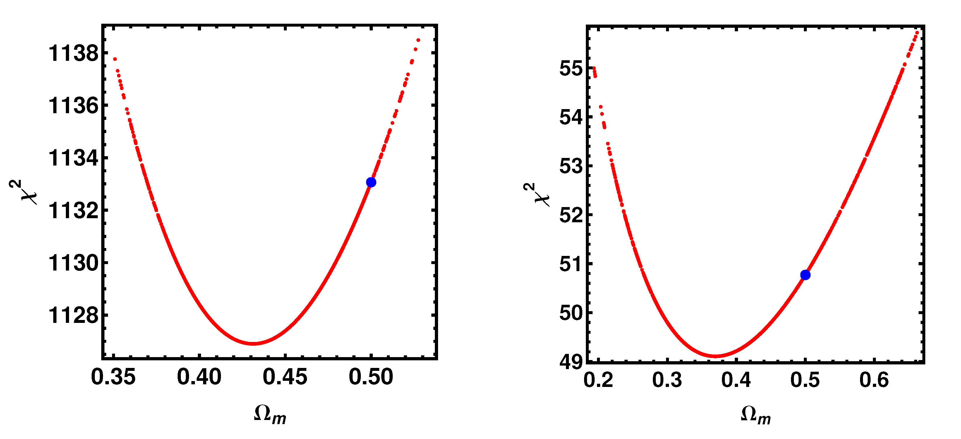
4. Results from Cosmological Fits

I here portray our theoretical scenarios that I am going to test with GRB data. I thus consider a generic version of the Hubble rate, taking pressureless matter with negligible contribution from radiation and spatial curvature, i.e., imposing Ω k = 0 [52].
I handle a DE field with the equation of state P = w ρ , with constant w. This approach involves two models of particular interest: the first, the concordance paradigm, is defined as w 1 , whereas the second takes w < 0 with no further impositions. In particular, I write
H ( z ) = H 0 Ω m ( 1 + z ) 3 + Ω DE ( 1 + z ) 3 ( 1 + w ) ,
where the matter density is defined by Ω m = ρ m / ρ c with ρ c 8 π G / ( 3 H 0 2 ) the critical density. The DE cosmological parameter becomes Ω DE = 1 Ω m , being w the DE parameter. In particular, Equation (11) results in the Λ CDM model for w 1 , or else to the wCDM model.
To search for the best-fit parameters of the above cosmological models, I perform a MCMC numerical integration on the χ 2 distribution by means of the Metropolis-Hastings algorithm implemented on a Mathematica code. This code starts by assuming priors on the fitting parameters and fixing H 0 = 67.74 km s 1 Mpc 1 as indicated in the Section 1; the search of the best-fit proceeds by using a random walk behaviour through 10 4 steps searches for the set of model parameters minimizing the χ 2 .

4.1. The  Λ CDM Model

To get the Λ CDM (for a different perspective, see [53]), I set w = 1 in Equation (11), leaving Ω m the only parameter to be found by the MCMC simulation. At this stage I employ GRB data alone to obtain constraints on Ω m from the minimization of the Amati/Combo relation chi square
χ A / C 2 = i = 1 N A / C μ A / C , i μ GRB th Ω m , z i σ μ A / C , i 2 ,
where for the Amati correlation N A = 193 and for the Combo correlation N C = 60 ; μ GRB th is the theoretical GRB distance modulus computed from a given model. For the MCMC simulations, I assume the uniform prior 0 Ω m 1 . The fit results for the Λ CDM model are shown in Figure 4 and summarized in Table 1.
Now, I perform a fit within the Λ CDM model, including the distance moduli from the SNe Ia Pantheon Sample, the largest combined sample consisting of 1048 sources Ia ranging from 0.01 < z < 2.3 [37]. The SN Ia distance modulus is given by
μ SN = m B M α X 1 + β C Δ M Δ B ,
and depends upon the The B-band apparent m B and absolute M magnitudes, the stretch X 1 and colour C light curve factors, the luminosity-stretch α and luminosity-color β parameters, and, finally, the distance corrections Δ M , based on the host galaxy mass of the SN, and Δ B , based on predicted biases from simulations. M does not enter the SN uncertainties, thus, the SN chi-square is
χ SN 2 = Δ μ SN M 1 T C 1 Δ μ SN M 1 ,
where Δ μ SN μ SN μ SN th Ω m , z i is the vector of residuals, and The covariance matrix C accounts for statistical and systematic uncertainties [54]. By analytically marginalizing over M through a flat prior [55], the SN chi-square becomes independent from it, leading to
χ SN , M 2 = a + log e 2 π b 2 e ,
in which a Δ μ SN T C 1 Δ μ SN , b Δ μ SN T C 1 1 , and e 1 T C 1 1 . Analytical marginalizations over α and β are not possible, because they enter in the SN uncertainties.
The total chi-square for the Λ CDM is thus given by
χ 2 Ω m = χ A / C 2 Ω m + χ SN , M 2 Ω m ,
and it is computed for each GRB correlation. For the MCMC simulations, I assume the same uniform priors as for the above fit involving GRB data alone. The fit results are shown in Figure 5 and summarized in Table 1.

4.2. The wCDM Model

Now, I perform fits using the wCDM model, obtained from Equation (11) by allowing the w parameter free to vary. Hence, the model parameters to be found by the MCMC simulation are now w and Ω m . In this case the use of GRB data alone does not provide acceptable constraints on w. Therefore, to obtain more robust bounds on this parameter , I make use of the combined GRB+SN sample.
The total chi-square for the wCDM model
χ w 2 Ω m , w = χ A / C 2 Ω m , w + χ SN , M 2 Ω m , w
is computed for each GRB correlation and using μ GRB th Ω m , w , z i and μ SN th Ω m , w , z i . For the MCMC simulations, I assume the uniform priors 0 Ω m 1 and 3 w 0 . The fit results for the wCDM model are shown in Figure 6 and summarized in Table 1.

4.3. Results

From the fits on the Λ CDM obtained by employing GRB datasets alone, summarized in Table 1 and portrayed in Figure 4, one immediately notices that Ω m is higher when compared to the results from other surveys [19,20,29,30,32,56]. This discrepancy tends to be flattened for both Λ CDM and wCDM models, when including SN Ia dataset (see Table 1 and Figure 5 and Figure 6).
Going into details for the Amati correlation, the results from the Λ CDM model are in tension with Planck predictions [52] at a confidence level 3 σ , but consistent within 1– σ with previous results obtained from GRB data alone [19,20,29,30,32,56]. As stated above, this tension is slightly reduced by including SN Ia dataset. Λ CDM and wCDM best-fit models obtained by considering GRB+SN datasets have the same number of datapoints and just one degree of freedom (DoF) of difference (see Table 1). From their direct comparison, one can see that the wCDM model leads to a modest improvements in the χ 2 by introducing an extra parameter. Moreover the w parameter is consistent within 1– σ with the Λ CDM case, i.e., w = 1 . This represents a clear indication that, from a statistical point of view, the Λ CDM model is a better fit than the wCDM one to fit the SN+Amati GRB dataset.
For the Combo correlation, the results from both Λ CDM and wCDM models are consistent with Planck predictions [52] within 1– σ . Also in this case, from The direct comparison between the best-fit results, the Λ CDM model is a better fit than the wCDM one to fit the SN+Combo GRB dataset.
By sorting the correlations by the χ 2 / DoF values, one notices immediately that this ratio for Combo relation is smaller and closer to unity than the Amati one. At this stage it is not clear whether these findings are due to the fact that the Combo GRB dataset is smaller than the Amati one, leading to larger attached errors, or because the Combo correlation is indeed a more suited correlation for cosmological analyses. Future updates on both datasets may shed light on this issue and strengthen the statistical contents for both correlations.
It is worth to mention that the results listed in Table 1 and displayed in Figure 4, Figure 5 and Figure 6 slightly differ to (though are consistent with) those obtained in Ref. [32] by employing Amati GRBs and SNe Ia. The reason for this difference has to be seeked in the different SN Ia sample used here (The Pantheon dataset) and that employed in Ref. [32] (The JLA dataset). In any case, as expected, the results are consistent at 1– σ confidence level.

5. Conclusions and Discussions

I employ a new method, based on the approximation of the OHD data with Beziér polynomials [32], to calibrate in a cosmology-independent way two GRB correlations: Amati and Combo. Through this technique, GRB distance moduli have been obtained without postulating an a priori cosmological model and just imputing the information on curvature Ω k = 0 from Planck [52]. In such a way the circularity problem affecting GRB correlations has been healed.
From the model-independently calibrated Amati and Combo correlations I performed MCMC analyses: in a first set of simulations, I tested the Λ CDM model by using (a) GRB data alone and (b) GRB data and SNe Ia from the Pantheon sample [37]; in a second set, I tested the wCDM model by considering only GRB+SN datasets, because GRBs alone do not provide acceptable constraints on w.
The results of the MCMC simulations are summarized in Table 1 and portrayed in Figure 4, Figure 5 and Figure 6. Though consistent within 1– σ with previous results obtained from GRB data alone [19,20,29,30,32,56], the results from the Amati correlation are in tension with Planck predictions [52] at a confidence level 3 σ for both Λ CDM and wCDM models. This findings are somewhat in line with recent claims on tensions with the Λ CDM model [57,58]. However, while the value of Ω m is always noticeably high, within The wCDM model the value of the w parameter is consistent within 1– σ with the Λ CDM case, i.e., w = 1 . The results obtained for the Amati correlation case slightly differ to (though are consistent at 1– σ confidence level with) those obtained in Ref. [32]. This is likely due to different employed SN Ia samples, the Pantheon dataset used here and the JLA dataset employed in Ref. [32]. For the Combo correlation, all MCMC simulations give best-fit parameters which are consistent within 1– σ with the Λ CDM model. From a statistical significance point of view, the Amati correlation has the largest dataset; however, the Combo correlation provides the smaller values of the ratio χ 2 / DoF. At this stage it is not clear whether the diversity of the results from the two calibrated correlations is statistical, due to the difference in the dataset size of the correlations, or astrophysical, which may help in principle in establishing the most suited correlation for cosmological analyses. However, this can be an indication that more refined analyses are needed. The increase of both datasets may shed light on the above issues and strengthen the predictive power of both correlations.
Future perspectives of this work may shed light also on the role of spatial curvature. Recent literature raises doubts about fixing the spatial curvature to zero and claims that Ω k 0 , though it is very small [59], or that the current constraint Ω k = 0.001 ± 0.002 [52] is based on the pre-assumption of a flat surface in a DE analysis [60]. However, by relaxing the assumption Ω k = 0 , the circularity problem is not fully healed since the luminosity distance in Equation (2) depends upon Ω k . This implies that quantities such as E iso and L 0 are now functions of Ω k . Therefore, in order to measure the curvature parameter, one may still employ the model-independent method based on Bézier polynomials to approximate the OHD data with the function H 2 ( z ) , use it in the luminosity distance definition, and jointly fit Ω k with the GRB correlation best-fit parameters [60].
Finally, the results obtained in this work are in line with w = 1 and a cosmological constant Λ describing the DE evolution, as purported by the Λ CDM model. At this stage, slow and/or small DE evolution with time, cannot be excluded. On The contrary, these numerical bounds seem to rule out barotropic DE models with fast variation of w at intermediate redshifts, such as all modified Chaplygin gas models, a few Cardassian universes, Braneworld cosmologies, etc. Concerning extended theories of gravity [48,51,61], provided their overall agreement with the above results, they cannot be excluded a priori. As stated above, this picture may change by exploring the possibility that there is non-zero curvature and may open new scenarios for the DE equation of state and evolution.

Funding

This research received no external funding.

Acknowledgments

I acknowledge the support of the project Iniziative Specifiche MOONLIGHT-2 at INFN-LNF. This work is dedicated to the memory of Diego Leonardo Caceres Uribe.

Conflicts of Interest

The author declares no conflict of interest.

References

  1. Phillips, M.M. The absolute magnitudes of Type IA supernovae. Astrophys. J. 1993, 413, L105–L108. [Google Scholar] [CrossRef]
  2. Perlmutter, S.; Aldering, G.; della Valle, M.; Deustua, S.; Ellis, R.S.; Fabbro, S.; Fruchter, A.; Goldhaber, G.; Groom, D.E.; Hook, I.M.; et al. Discovery of a supernova explosion at half the age of the universe. Nature 1998, 391, 51. [Google Scholar] [CrossRef] [Green Version]
  3. Riess, A.G.; Filippenko, A.V.; Challis, P.; Clocchiatti, A.; Diercks, A.; Garnavich, P.M.; Gilliland, R.L.; Hogan, C.J.; Jha, S.; Kirshner, R.P.; et al. Observational Evidence from Supernovae for an Accelerating Universe and a Cosmological Constant. Astron. J. 1998, 116, 1009–1038. [Google Scholar] [CrossRef] [Green Version]
  4. Schmidt, B.P.; Suntzeff, N.B.; Phillips, M.M.; Schommer, R.A.; Clocchiatti, A.; Kirshner, R.P.; Garnavich, P.; Challis, P.; Leibundgut, B.; Spyromilio, J.; et al. The High-Z Supernova Search: Measuring Cosmic Deceleration and Global Curvature of the Universe Using Type IA Supernovae. Astrophys. J. 1998, 507, 46–63. [Google Scholar] [CrossRef]
  5. Kang, Y.; Lee, Y.W. Investigation of Stellar Populations in the Early type Host Galaxies of Type Ia Supernovae. Am. Astron. Soc. Meet. Abstr. 2019, 233, 312.03. [Google Scholar]
  6. Rodney, S.A.; Riess, A.G.; Scolnic, D.M.; Jones, D.O.; Hemmati, S.; Molino, A.; McCully, C.; Mobasher, B.; Strolger, L.G.; Graur, O.; et al. Two SNe Ia at Redshift ∼2: Improved Classification and Redshift Determination with Medium-band Infrared Imaging. Astron. J. 2015, 150, 156. [Google Scholar] [CrossRef] [Green Version]
  7. Aviles, A.; Gruber, C.; Luongo, O.; Quevedo, H. Cosmography and constraints on the equation of state of the Universe in various parametrizations. Phys. Rev. D 2012, 86, 123516. [Google Scholar] [CrossRef] [Green Version]
  8. Capozziello, S.; D’Agostino, R.; Luongo, O. Extended gravity cosmography. Int. J. Mod. Phys. D 2019, 28, 1930016. [Google Scholar] [CrossRef] [Green Version]
  9. Capozziello, S.; De Laurentis, M.; Luongo, O.; Ruggeri, A. Cosmographic Constraints and Cosmic Fluids. Galaxies 2013, 1, 216–260. [Google Scholar] [CrossRef] [Green Version]
  10. Luongo, O.; Battista Pisani, G.; Troisi, A. Cosmological degeneracy versus cosmography: A cosmographic dark energy model. arXiv 2015, arXiv:1512.07076. [Google Scholar] [CrossRef] [Green Version]
  11. Salvaterra, R.; Della Valle, M.; Campana, S.; Chincarini, G.; Covino, S.; D’Avanzo, P.; Fernández-Soto, A.; Guidorzi, C.; Mannucci, F.; Margutti, R.; et al. GRB090423 at a redshift of z˜8.1. Nature 2009, 461, 1258. [Google Scholar] [CrossRef] [PubMed] [Green Version]
  12. Tanvir, N.R.; Fox, D.B.; Levan, A.J.; Berger, E.; Wiersema, K.; Fynbo, J.P.U.; Cucchiara, A.; Krühler, T.; Gehrels, N.; Bloom, J.S.; et al. A γ-ray burst at a redshift of z˜8.2. Nature 2009, 461, 1254. [Google Scholar] [CrossRef] [PubMed] [Green Version]
  13. Cucchiara, A.; Levan, A.J.; Fox, D.B.; Tanvir, N.R.; Ukwatta, T.N.; Berger, E.; Krühler, T.; Küpcü Yoldaş, A.; Wu, X.F.; Toma, K.; et al. A Photometric Redshift of z˜9.4 for GRB 090429B. Astrophys. J. 2011, 736, 7. [Google Scholar] [CrossRef] [Green Version]
  14. Salvaterra, R.; Campana, S.; Vergani, S.D.; Covino, S.; D’Avanzo, P.; Fugazza, D.; Ghirlanda, G.; Ghisellini, G.; Melandri, A.; Nava, L.; et al. A Complete Sample of Bright Swift Long Gamma-Ray Bursts. I. Sample Presentation, Luminosity Function and Evolution. Astrophys. J. 2012, 749, 68. [Google Scholar] [CrossRef]
  15. Coward, D.M.; Howell, E.J.; Branchesi, M.; Stratta, G.; Guetta, D.; Gendre, B.; Macpherson, D. The Swift gamma-ray burst redshift distribution: Selection biases and optical brightness evolution at high z? Mon. Not. R. Astron. Soc. 2013, 432, 2141–2149. [Google Scholar] [CrossRef]
  16. Amati, L. The Ep,i-Eiso correlation in gamma-ray bursts: Updated observational status, re-analysis and main implications. Mon. Not. R. Astron. Soc. 2006, 372, 233–245. [Google Scholar] [CrossRef] [Green Version]
  17. Ghirlanda, G.; Ghisellini, G.; Firmani, C. Gamma-ray bursts as standard candles to constrain the cosmological parameters. New J. Phys. 2006, 8, 123. [Google Scholar] [CrossRef]
  18. Nava, L.; Salvaterra, R.; Ghirlanda, G.; Ghisellini, G.; Campana, S.; Covino, S.; Cusumano, G.; D’Avanzo, P.; D’Elia, V.; Fugazza, D.; et al. A complete sample of bright Swift long gamma-ray bursts: Testing the spectral-energy correlations. Mon. Not. R. Astron. Soc. 2012, 421, 1256–1264. [Google Scholar] [CrossRef] [Green Version]
  19. Amati, L.; Della Valle, M. Measuring Cosmological Parameters with Gamma Ray Bursts. Int. J. Mod. Phys. D 2013, 22, 1330028. [Google Scholar] [CrossRef] [Green Version]
  20. Demianski, M.; Piedipalumbo, E.; Sawant, D.; Amati, L. Cosmology with gamma-ray bursts. I. the Hubble diagram through the calibrated Ep,i-Eiso correlation. Astron. Astrophys. 2017, 598, A112. [Google Scholar] [CrossRef] [Green Version]
  21. Amati, L.; Frontera, F.; Tavani, M.; in’t Zand, J.J.M.; Antonelli, A.; Costa, E.; Feroci, M.; Guidorzi, C.; Heise, J.; Masetti, N.; et al. Intrinsic spectra and energetics of BeppoSAX Gamma-Ray Bursts with known redshifts. Astron. Astrophys. 2002, 390, 81. [Google Scholar] [CrossRef]
  22. Ghirlanda, G.; Ghisellini, G.; Lazzati, D.; Firmani, C. Gamma-Ray Bursts: New Rulers to Measure the Universe. Astrophys. J. 2004, 613, L13–L16. [Google Scholar] [CrossRef]
  23. Amati, L.; Guidorzi, C.; Frontera, F.; Della Valle, M.; Finelli, F.; Landi, R.; Montanari, E. Measuring the cosmological parameters with the Ep,iEiso correlation of gamma-ray bursts. Mon. Not. R. Astron. Soc. 2008, 391, 577. [Google Scholar] [CrossRef] [Green Version]
  24. Schaefer, B.E. The Hubble Diagram to Redshift > 6 from 69 Gamma-Ray Bursts. Astrophys. J. 2007, 660, 16. [Google Scholar] [CrossRef] [Green Version]
  25. Capozziello, S.; Izzo, L. Cosmography by gamma ray bursts. Astron. Astrophys. 2008, 490, 31–36. [Google Scholar] [CrossRef] [Green Version]
  26. Dainotti, M.G.; Cardone, V.F.; Capozziello, S. A time-luminosity correlation for γ-ray bursts in the X-rays. Mon. Not. R. Astron. Soc. 2008, 391, L79–L83. [Google Scholar] [CrossRef]
  27. Bernardini, M.G.; Margutti, R.; Zaninoni, E.; Chincarini, G. A universal scaling for short and long gamma-ray bursts: EX,iso-Eγ,iso-Epk. Mon. Not. R. Astron. Soc. 2012, 425, 1199–1204. [Google Scholar] [CrossRef] [Green Version]
  28. Wei, J.J.; Wu, X.F.; Melia, F.; Wei, D.M.; Feng, L.L. Cosmological tests using gamma-ray bursts, the star formation rate and possible abundance evolution. Mon. Not. R. Astron. Soc. 2014, 439, 3329–3341. [Google Scholar] [CrossRef]
  29. Izzo, L.; Muccino, M.; Zaninoni, E.; Amati, L.; Della Valle, M. New measurements of Ωm from gamma-ray bursts. Astron. Astrophys. 2015, 582, A115. [Google Scholar] [CrossRef] [Green Version]
  30. Demianski, M.; Piedipalumbo, E.; Sawant, D.; Amati, L. Cosmology with gamma-ray bursts. II. Cosmography challenges and cosmological scenarios for the accelerated Universe. Astron. Astrophys. 2017, 598, A113. [Google Scholar] [CrossRef]
  31. Kodama, Y.; Yonetoku, D.; Murakami, T.; Tanabe, S.; Tsutsui, R.; Nakamura, T. Gamma-ray bursts in 1.8 < z < 5.6 suggest that the time variation of the dark energy is small. Mon. Not. R. Astron. Soc. 2008, 391, L1–L4. [Google Scholar] [CrossRef] [Green Version]
  32. Amati, L.; D’Agostino, R.; Luongo, O.; Muccino, M.; Tantalo, M. Addressing the circularity problem in the Ep-Eiso correlation of gamma-ray bursts. Mon. Not. R. Astron. Soc. 2019, 486, L46–L51. [Google Scholar] [CrossRef] [Green Version]
  33. Dainotti, M.G.; Amati, L. Gamma-ray Burst Prompt Correlations: Selection and Instrumental Effects. Publ. Astron. Soc. Pac. 2018, 130, 051001. [Google Scholar] [CrossRef] [Green Version]
  34. Jimenez, R.; Loeb, A. Constraining Cosmological Parameters Based on Relative Galaxy Ages. Astrophys. J. 2002, 573, 37–42. [Google Scholar] [CrossRef]
  35. Capozziello, S.; D’Agostino, R.; Luongo, O. Cosmographic analysis with Chebyshev polynomials. Mon. Not. R. Astron. Soc. 2018, 476, 3924–3938. [Google Scholar] [CrossRef] [Green Version]
  36. Montiel, A.; Cabrera, J.I.; Hidalgo, J.C. Improving sampling and calibration of GRBs as distance indicators. arXiv 2020, arXiv:2003.03387. [Google Scholar]
  37. Scolnic, D.M.; Jones, D.O.; Rest, A.; Pan, Y.C.; Chornock, R.; Foley, R.J.; Huber, M.E.; Kessler, R.; Narayan, G.; Riess, A.G.; et al. The Complete Light-curve Sample of Spectroscopically Confirmed SNe Ia from Pan-STARRS1 and Cosmological Constraints from the Combined Pantheon Sample. Astrophys. J. 2018, 859, 101. [Google Scholar] [CrossRef]
  38. Betoule, M.; Kessler, R.; Guy, J.; Mosher, J.; Hardin, D.; Biswas, R.; Astier, P.; El-Hage, P.; Konig, M.; Kuhlmann, S.; et al. Improved cosmological constraints from a joint analysis of the SDSS-II and SNLS supernova samples. Astron. Astrophys. 2014, 568, A22. [Google Scholar] [CrossRef]
  39. Liang, N.; Xiao, W.K.; Liu, Y.; Zhang, S.N. A Cosmology-Independent Calibration of Gamma-Ray Burst Luminosity Relations and the Hubble Diagram. Astrophys. J. 2008, 685, 354–360. [Google Scholar] [CrossRef] [Green Version]
  40. Luongo, O. Cosmography with the Hubble Parameter. Mod. Phys. Lett. A 2011, 26, 1459–1466. [Google Scholar] [CrossRef]
  41. Aviles, A.; Bravetti, A.; Capozziello, S.; Luongo, O. Updated constraints on f(R) gravity from cosmography. Phys. Rev. D 2013, 87, 044012. [Google Scholar] [CrossRef] [Green Version]
  42. Aviles, A.; Bravetti, A.; Capozziello, S.; Luongo, O. Cosmographic reconstruction of f(T) cosmology. Phys. Rev. D 2013, 87, 064025. [Google Scholar] [CrossRef] [Green Version]
  43. Luongo, O. Dark Energy from a Positive Jerk Parameter. Mod. Phys. Lett. A 2013, 28, 1350080. [Google Scholar] [CrossRef]
  44. Gruber, C.; Luongo, O. Cosmographic analysis of the equation of state of the universe through Padé approximations. Phys. Rev. D 2014, 89, 103506. [Google Scholar] [CrossRef] [Green Version]
  45. Capozziello, S.; Farooq, O.; Luongo, O.; Ratra, B. Cosmographic bounds on the cosmological deceleration-acceleration transition redshift in f(R) gravity. Phys. Rev. D 2014, 90, 044016. [Google Scholar] [CrossRef] [Green Version]
  46. Aviles, A.; Bravetti, A.; Capozziello, S.; Luongo, O. Precision cosmology with Padé rational approximations: Theoretical predictions versus observational limits. Phys. Rev. D 2014, 90, 043531. [Google Scholar] [CrossRef] [Green Version]
  47. Capozziello, S.; Luongo, O.; Saridakis, E.N. Transition redshift in f (T ) cosmology and observational constraints. Phys. Rev. D 2015, 91, 124037. [Google Scholar] [CrossRef]
  48. de la Cruz-Dombriz, Á.; Dunsby, P.K.S.; Luongo, O.; Reverberi, L. Model-independent limits and constraints on extended theories of gravity from cosmic reconstruction techniques. J. Cosmol. Astropart. Phys. 2016, 2016, 042. [Google Scholar] [CrossRef] [Green Version]
  49. Capozziello, S.; D’Agostino, R.; Luongo, O. Model-independent reconstruction of f( T) teleparallel cosmology. Gen. Relativ. Gravit. 2017, 49, 141. [Google Scholar] [CrossRef] [Green Version]
  50. Calzá, M.; Casalino, A.; Luongo, O.; Sebastiani, L. Kinematic reconstructions of extended theories of gravity at small and intermediate redshifts. Eur. Phys. J. Plus 2020, 135, 1. [Google Scholar] [CrossRef]
  51. Capozziello, S.; D’Agostino, R.; Luongo, O. High-redshift cosmography: Auxiliary variables versus Padé polynomials. Mon. Not. R. Astron. Soc. 2020, 494, 2576–2590. [Google Scholar] [CrossRef]
  52. Planck Collaboration; Aghanim, N.; Akrami, Y.; Ashdown, M.; Aumont, J.; Baccigalupi, C.; Ballardini, M.; Banday, A.J.; Barreiro, R.B.; Bartolo, N.; et al. Planck 2018 results. VI. Cosmological parameters. arXiv 2019, arXiv:1807.06209. [Google Scholar]
  53. Luongo, O.; Muccino, M. Speeding up the Universe using dust with pressure. Phys. Rev. D 2018, 98, 103520. [Google Scholar] [CrossRef] [Green Version]
  54. Conley, A.; Guy, J.; Sullivan, M.; Regnault, N.; Astier, P.; Balland, C.; Basa, S.; Carlberg, R.G.; Fouchez, D.; Hardin, D.; et al. Supernova Constraints and Systematic Uncertainties from the First Three Years of the Supernova Legacy Survey. ApJS 2011, 192, 1. [Google Scholar] [CrossRef]
  55. Goliath, M.; Amanullah, R.; Astier, P.; Goobar, A.; Pain, R. Supernovae and the nature of the dark energy. Astron. Astrophys. 2001, 380, 6–18. [Google Scholar] [CrossRef]
  56. Haridasu, B.S.; Luković, V.V.; D’Agostino, R.; Vittorio, N. Strong evidence for an accelerating universe. Astron. Astrophys. 2017, 600, L1. [Google Scholar] [CrossRef]
  57. Yang, T.; Banerjee, A.; Colgáin, E.Ó. On cosmography and flat ΛCDM tensions at high redshift. arXiv 2019, arXiv:1911.01681. [Google Scholar]
  58. Risaliti, G.; Lusso, E. Cosmological Constraints from the Hubble Diagram of Quasars at High Redshifts. Nat. Astron. 2019, 3, 272–277. [Google Scholar] [CrossRef] [Green Version]
  59. Ooba, J.; Ratra, B.; Sugiyama, N. Planck 2015 Constraints on the Non-flat ΛCDM Inflation Model. Astrophys. J. 2018, 864, 80. [Google Scholar] [CrossRef] [Green Version]
  60. Wei, J.J.; Melia, F. Model-independent Distance Calibration and Curvature Measurement Using Quasars and Cosmic Chronometers. Astrophys. J. 2020, 888, 99. [Google Scholar] [CrossRef] [Green Version]
  61. Capozziello, S.; D’Agostino, R.; Luongo, O. Kinematic model-independent reconstruction of Palatini f(R) cosmology. Gen. Relativ. Gravit. 2019, 51, 2. [Google Scholar] [CrossRef] [Green Version]
Figure 1. OHD best-fit (solid thick blue) line (black points) with its 1– σ (light blue shaded area) and 3– σ (blue dashed curves) confidence regions. Reproduced from Ref. [32].
Symmetry 12 01118 g001
Figure 2. Left: the calibrated E p E iso correlation (black data), the best-fitting function (blue solid line) and the 1 σ A and 3 σ A limits (dark-gray and light-gray shaded regions, respectively). Right: the distribution of the GRB distance moduli μ A as obtained from the calibrated Amati correlation. Reproduced from Ref. [32].
Symmetry 12 01118 g002
Figure 3. Left: the calibrated Combo correlation (black data), the best-fit (red solid line) and the 1 σ C and 3 σ C limits (dark-orange and light-orange shaded regions, respectively). Right: the distribution of the GRB distance moduli μ C as obtained from the calibrated Combo correlation.
Symmetry 12 01118 g003
Figure 4. Plots of the χ A / C 2 distribution (red points) from the MCMC simulation for the Λ CDM model. Left: the χ A 2 of the Amati correlation; right: the χ C 2 of the Combo correlation. The blue points represent the starting point of the MCMC simulation.
Symmetry 12 01118 g004
Figure 5. Plots of the χ 2 distribution (red points) from the MCMC simulation for the Λ CDM model. Left: Amati GRB+SN dataset; right: Combo GRB+SN dataset. The blue points represent the starting point of the MCMC simulation.
Symmetry 12 01118 g005
Figure 6. Ω m w contour plots for the wCDM model obtained from SNe+Amati GRBs (left), and SNe+Combo GRBs (right). Black dots represent the best-fit values; the 1- and 2– σ contours are displayed, from The inner/darker to the outer/lighter areas.
Symmetry 12 01118 g006
Table 1. Best-fit results and errors at 1- σ (3– σ ) confidence level of the MCMC simulation for the  Λ CDM model, with both GRB and GRB+SN samples, and The wCDM model, with GRB+SN sample. The  χ 2 / DoF ratios are also indicated.
SampleAmatiCombo
w Ω m χ 2 / DoFw Ω m χ 2 / DoF
ΛCDM
GRB 1 0.43 0.03 ( 0.07 ) + 0.03 ( + 0.09 ) 1126.9 / 192 1 0.37 0.08 ( 0.19 ) + 0.08 ( + 0.22 ) 49.1 / 59
GRB+SN 1 0.36 0.01 ( 0.05 ) + 0.02 ( + 0.05 ) 2177.0 / 1240 1 0.30 0.02 ( 0.06 ) + 0.02 ( + 0.07 ) 1084.5 / 1107
wCDM
GRB+SN 1.15 0.20 ( 0.60 ) + 0.16 ( + 0.45 ) 0.40 0.04 ( 0.15 ) + 0.04 ( + 0.10 ) 2176.3 / 1239 1.12 0.26 ( 0.77 ) + 0.15 ( + 0.38 ) 0.34 0.04 ( 0.16 ) + 0.06 ( + 0.16 ) 1084.2 / 1106

