UAV Group Formation Collision Avoidance Method Based on Second-Order Consensus Algorithm and Improved Artificial Potential Field

Abstract

The problem of collision avoidance of an unmanned aerial vehicle (UAV) group is studied in this paper. A collision avoidance method of UAV group formation based on second-order consensus algorithm and improved artificial potential field is proposed. Based on the method, the UAV group can form a predetermined formation from any initial state and fly to the target position in normal flight, and can avoid collision according to the improved smooth artificial potential field method when encountering an obstacle. The UAV group adopts the “leader–follower” strategy, that is, the leader UAV is the controller and flies independently according to the mission requirements, while the follower UAV follows the leader UAV based on the second-order consensus algorithm and formations gradually form during the flight. Based on the second-order consensus algorithm, the UAV group can achieve formation maintenance easily and the Laplacian matrix used in the algorithm is symmetric for an undirected graph. In the process of obstacle avoidance, the improved artificial potential field method can solve the jitter problem that the traditional artificial potential field method causes for the UAV and avoids violent jitter. Finally, simulation experiments of two scenarios were designed to verify the collision avoidance effect and formation retention effect of static obstacles and dynamic obstacles while the two UAV groups fly in opposite symmetry in the dynamic obstacle scenario. The experimental results demonstrate the effectiveness of the proposed method.

1. Introduction

Group control issues have long been recognized as a very important part of a multi-agent system. Because in the near future, it will become more and more common for unmanned robots to replace people in a cluster to perform difficult tasks. Cluster phenomena are common in nature, such as flocks, ant colonies, bee colonies and so on. These phenomena have inspired us to study the behavior of these biological groups to control unmanned clusters [1,2,3,4]. The way unmanned aerial vehicles (UAVs) perform tasks are becoming more and more clustered. Formation maintenance is one of the key technologies of UAV cluster technology. At the same time, collision avoidance technology is also the basic problem to be considered in cluster control [5,6]. In response to those problems, this paper studies and analyzes the collision avoidance technology in the case of formation maintenance.

Cluster avoidance is studied via cluster formation control, mainly through the graph theory method and the Laplace function method. Among them, the degree matrix, the adjacency matrix and the Laplacian matrix are very commonly used in the graph theory control method [7]. The eigenvalues of the Laplacian matrix can reflect much of the information of the network. Literature [8] clearly discusses the stability of formation topology represented by undirected graphs, and points out that the study of graphs plays a key role in formation control. The minimum positive eigenvalue of the Laplacian matrix determines the time it takes for the agent to reach the formation position. However, the complex analysis of the switching network topology makes the applicability of these attributes very difficult [9]. The Laplace function method is the most advantageous method for the stability analysis of complex dynamic systems and control theory, because, for the analysis of nonlinear systems, it is easier to use Laplacian functions rather than matrix theory methods [9]. A very important aspect of cluster control is consensus. Consensus means that each individual in the cluster reaches a common indicator according to an algorithm to maintain a stable state [10]. In the actual scenario, the consensus of cluster control is mainly reflected in the control of the formation under the consensus strategy. The formation control mainly hopes that all the agents in the formation can maintain a stable formation. Therefore, the strategy based on distance maintenance is more suitable for practical use because it does not require harsh sensitivity. This idea is representative of the self-organizing agent consensus algorithm [11]. A necessary and sufficient condition for reaching a consensus is that the communication directed graph allows for a directed spanning tree [10,11]. The literature [12,13] only proves sufficiency and assumes that the graph is undirected or strongly connected.

Collision avoidance is an indispensable part while maintaining the formation of the UAV cluster. Collision avoidance includes collision avoidance against stationary obstacles and dynamic collision avoidance between UAV clusters. Traditional methods of collision avoidance include methods at the tactical level and methods at the strategic level [14]. The method at the tactical level is a collision avoidance algorithm based on geometric relations, mainly by analyzing geometric relations in space and provide conflict resolution [15,16,17,18]. The strategic level approach refers to proactively planning collision-free flight paths from the current location to the destination based on the perceptual detection of obstacles under the constraints of the minimum safe separation distance. Among them, the performance of systems using radar to actively detect obstacles is discussed in [19]. The collision avoidance algorithm based on geometric relationship has the characteristics of simple and efficient calculation, but most of the collision avoidance systems based on geometric relationship only support the collision avoidance between a pair of UAVs. At the same time, the method has strong requirements on the accuracy and real-time response of the sensor in actual use [20]. The main aspects of the trajectory planning algorithm at the strategic level include the potential field method [21,22,23], linear programming [24], and intelligent optimization algorithm [25]. The linear programming algorithm will significantly reduce computational efficiency with the increase of the number of UAVs. The intelligent optimization algorithm can quickly calculate the path, but the accuracy of its inherent properties is relatively low. The artificial potential field method has the characteristics of high computational efficiency and good real-time performance. It is widely used under real-time control conditions. The artificial potential field method was first proposed by Khatib, and its principle is very simple for real-time control [26,27]. However, the traditional artificial potential field method will have certain problems in practical application. The literature [22] combines the Lyapunov theorem with the artificial potential field method to solve the local minimum problem. [28] proposes a two-way concept and provides spacing information between UAVs so that they can avoid conflict in order to reach the target point. In [29], a new control force is proposed to transform the constrained UAV trajectory planning problem into an unconstrained UAV trajectory planning problem. The method proposed in this paper is based on the collision avoidance strategy of consensus strategy and artificial potential field method. Based on this method, the UAV cluster can quickly restore the formation while avoiding collision.

2. Consensus Algorithm

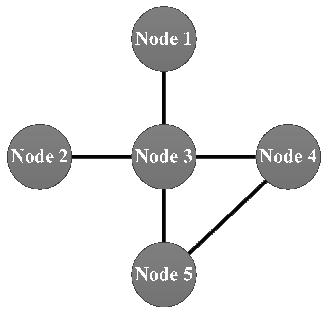
2.1. Graph Theory

This section introduces the basic concepts of graph theory and paves the way for subsequent formation consensus algorithms. The relationship between individuals in formation is represented by a weighted adjacency matrix. Suppose the nodes of the graph are $V=\{v_1,v_2,\dots ,v_N\}$, the directed edge are grouped $e={(E_{ij})}_{N\times N}$, and the weighted adjacency matrix is $d={(D_{ij})}_{N\times N}$. The directed edge $e_{ij}$ in the graph refers to the directed connection from node $v_i$ to node $v_j$.

The degree matrix is a diagonal matrix that represents the number of links each node connects to each node, represented by the following equation:

$$D_{i,j}=\{\begin{array}{c}\mathrm{deg}(v_i),\mathrm{if}i=j\\ 0,\mathrm{otherwise}\end{array}$$

(1)

The adjacency matrix represents the relationship between nodes and the relationship of information flow, which is represented by the following formula:

$$A_{i,j}=\{\begin{array}{c}1,\mathrm{if}j\mathrm{is}\mathrm{neighbor}\mathrm{of}i\\ 0,\mathrm{otherwise}\end{array}$$

(2)

The Laplacian matrix is: $L=D-A$. The eigenvalues of the Laplacian matrix are useful in many ways. The Laplacian matrix is also symmetric for an undirected graph and it is positive-semidefinite.

For instance, a graph with degree matrix, adjacency matrix and the Laplacian matrix is shown in Figure 1.

The degree matrix is written as:

$$D=\left[\begin{array}{ccccc}1& 0& 0& 0& 0\\ 0& 1& 0& 0& 0\\ 0& 0& 4& 0& 0\\ 0& 0& 0& 2& 0\\ 0& 0& 0& 0& 2\end{array}\right]$$

Adjacency matrix is:

$$A=\left[\begin{array}{ccccc}0& 0& 1& 0& 0\\ 0& 0& 1& 0& 0\\ 1& 1& 0& 1& 1\\ 0& 0& 1& 0& 1\\ 0& 0& 1& 1& 0\end{array}\right]$$

Laplacian matrix should be:

$$L=\left[\begin{array}{ccccc}1& 0& -1& 0& 0\\ 0& 1& -1& 0& 0\\ -1& -1& 4& -1& -1\\ 0& 0& -1& 2& -1\\ 0& 0& -1& -1& 2\end{array}\right]$$

The dynamic equation of the UAV is [7]:

$$\begin{array}{l}\dot{x}(t)=v(t)\\ \dot{v}(t)=a(t)\end{array}$$

(3)

where $x(0)=x_0,v(0)=v_0$, $x={[x_1^T,x_2^T,\dots ,x_n^T]}^T,v={[v_1^T,v_2^T,\dots ,v_n^T]}^T$. $x,v$ and $a$ are the position, velocity and acceleration of the UAV respectively.

The consensus clause is that the UAV needs to converge to the same state as the surrounding UAVs. In this paper, the formation maintenance is based on the second-order consensus. The second-order consensus is satisfied if the following formula can be satisfied [7]:

$$\begin{array}{l}{\Vert x_i(t)-x_j(t)\Vert }_{t\to \infty }=0\\ {\Vert v_i(t)-v_j(t)\Vert }_{t\to \infty }=0\end{array}$$

(4)

From Formulas (3) and (4), we can know that the second-order consensus can also be written as

$$\begin{array}{l}{\dot{x}}_i(t)={\dot{v}}_i(t)\\ {\dot{v}}_i(t)=-\omega {\displaystyle \sum _{j=1}^N{L}_{ij}{x}_j(t)-\phi {\displaystyle \sum _{j=1}^N{L}_{ij}{v}_j(t)}}\\ i=1,2,\dots ,N\end{array}$$

(5)

where $\omega$ and $\phi$ are constant.

Let $m={(x^T,v^T)}^T$, the above formula be written in a compact form [7]:

$$\dot{m}(t)=(L\otimes I_N)m$$

(6)

Among them $L$ is the Laplacian matrix, $\otimes$ is Kronecker multiplication.

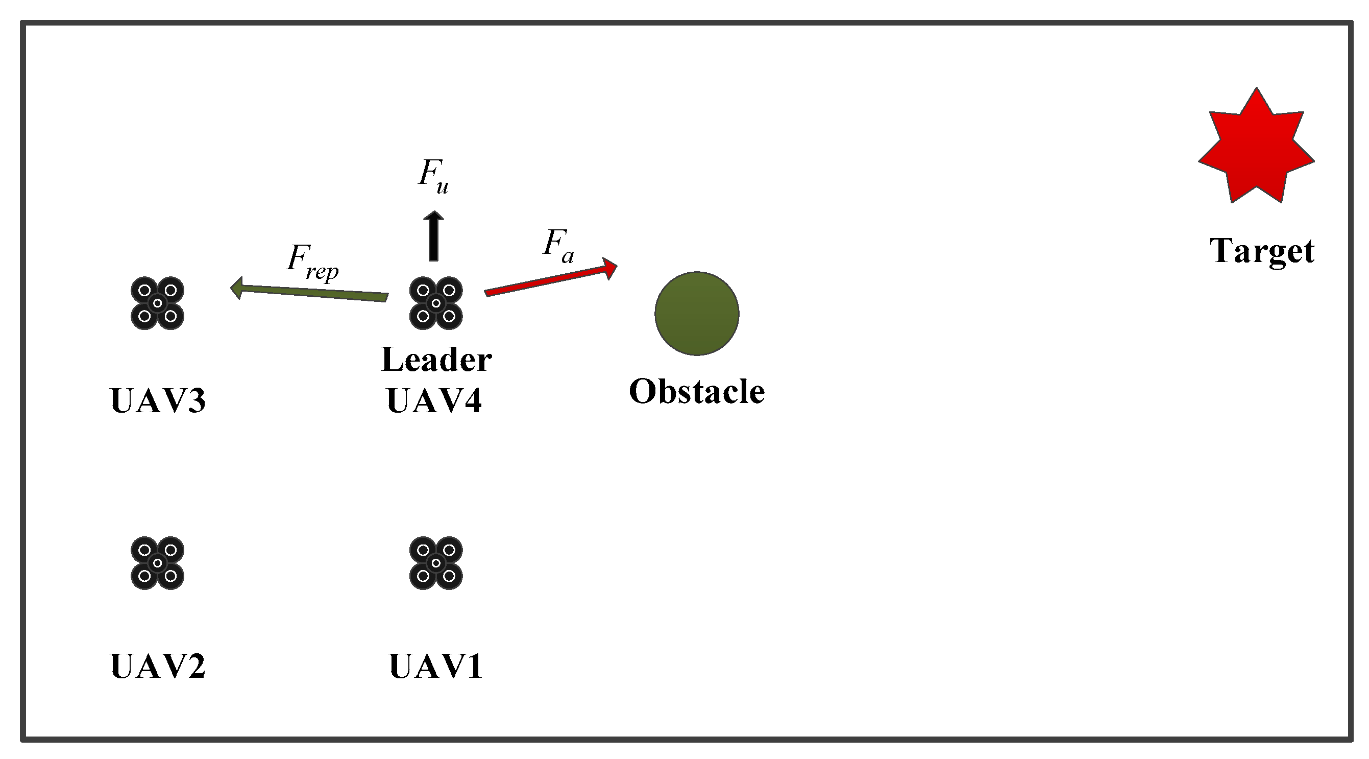
2.2. Artificial Potential Field Method

The paper adopts the adaptive artificial potential field method in the collision avoidance method of the UAV. The basic method is that the UAV moves in the direction in which the potential field drops at the fastest velocity [1]. The combined force of the attraction of the target and the repulsive force of the obstacle controls the next movement of the UAV.

Assuming that the position of the UAV is $P_{UAV}$, and the target position is $P_{goal}$, then the gravitational potential field function is [28]:

$$U_a={\zeta }_a{(P_{goal}-P_{UAV})}^2$$

(7)

The repulsion potential field function is [28]:

$$U_{rep}=\frac{1}{2}\psi {(\frac{1}{\lambda }-\frac{1}{{\lambda }_0})}^2$$

(8)

where ${\zeta }_a$ and $\psi$ are constants, $\lambda$ is the distance between the UAV and the obstacle. ${\lambda }_0$ is the maximum working distance between the UAV and the obstacle. When the relative distance is greater than the maximum working distance, the obstacle has no force on the UAV.

So the whole potential field is: $U_t=U_a+{\displaystyle \sum U_{rep}}$.

The algorithm has certain limitations. When the UAV approaches the obstacle, the repulsive force is significantly increased.

3. Second-Order Consensus Formation Control Model and Improved UAV Collision Avoidance Method

3.1. Formation Control Continuous Time Domain Model

Assume that each UAV meets the same dynamic equation:

$${\dot{s}}_i=K{s}_i+Z{a}_i,i=1,2,\dots ,N$$

(9)

where $s_i$ represents the amount of state that should be stored, $a_i$ represents the amount of control input. In order to control the position and velocity, $s_p=({(s_p)}_1,\dots ,{(s_p)}_{\mathrm{N}})$ and $s_v=({(s_v)}_1,\dots ,{(s_v)}_{\mathrm{N}})$ represent the position and velocity variables, so $s=s_p\otimes \left(\begin{array}{c}1\\ 0\end{array}\right)+s_v\otimes \left(\begin{array}{c}0\\ 1\end{array}\right)$. In this paper, in order to simplify the problem, we hypothesize $K=\left(\begin{array}{cc}0& 1\\ 0& 1\end{array}\right)$. This means that in this UAV dynamic system, the position of the UAV is determined only by the velocity, and the velocity is determined only by the amount of control input.

The formation is represented by the following vector $F=F_p\otimes \left(\begin{array}{c}1\\ 0\end{array}\right)\in R^{2nN}$, the UAV maintains a formation $F$ if and only if there is a vector $m,n\in R^n$ that satisfies ${(s_p)}_i(t)-{(F_p)}_i=m,{(s_p)}_i(t)=n,i=1,2,\dots ,N$ at the moment $t$. In the dynamic formation, the UAVs need to establish contact with each other to control the next movement of the UAV. This paper uses the Laplacian matrix to realize the formation control. Assume that ${\mathfrak{M}}_i$ is the neighbor of UAV $i$.

The output function can be defined as [13]:

$$z_i={\displaystyle \sum _{j={\mathfrak{M}}_j}((s_i-F_i)-(s_j-F_j)),i=1,\dots ,N}$$

(10)

The corresponding output vector can be written as $z=L(s-F)$, where $L$ is the Laplace matrix. After the formula is merged we can get [13]:

$$\begin{array}{l}\dot{s}=Kcs+Zca\\ a=L(s-F)\end{array}$$

(11)

where $Kc=I_N\otimes K,Zc=I_N\otimes Z$. The dynamic equation of the formation system in the continuous time domain is [7]:

$$\dot{s}=Kcs+ZcL(s-F)$$

(12)

3.2. Discretized Data Processing

The corresponding output vector can be written as $z=L(s-F)$, where $L$ is the Laplace matrix. After the formula is merged, you can get [7]:

$$\begin{array}{l}\dot{s}(t)=Ks(t)+Za(t)\\ m(t)=K_{1}s(t)+Z_{1}a(t)\end{array}$$

(13)

According to Formula (13), the state $s$ at the moment $(k+1)T$ can be obtained:

$$s((k+1)T)=e^{K(k+1)T}x(0)+e^{K(k+1)T}{\displaystyle {\int }_0^{(k+1)T}{e}^{-K\phi }Za(\phi )}d\phi$$

(14)

Set $Kd$ to the matrix $K$ in the discrete model, $Kd=e^{Kt}$. Available from Taylor’s expansion:

$$e^{Kt}=I+tK+\frac{1}{2!}{t}^2{K}^2+\frac{1}{3!}{t}^3{K}^3\dots ={\displaystyle \sum _{i=0}^{\infty }\frac{1}{i!}{t}^i{K}^i}$$

(15)

Remove the high-order items, we can get $Kd=I+tK$, $Zd={\displaystyle {\int }_0^t{e}^y}Zdy$. Then the discretization model of the continuous time domain is:

$$s((k+1)T)=Kds(kT)+Zda(kT)$$

(16)

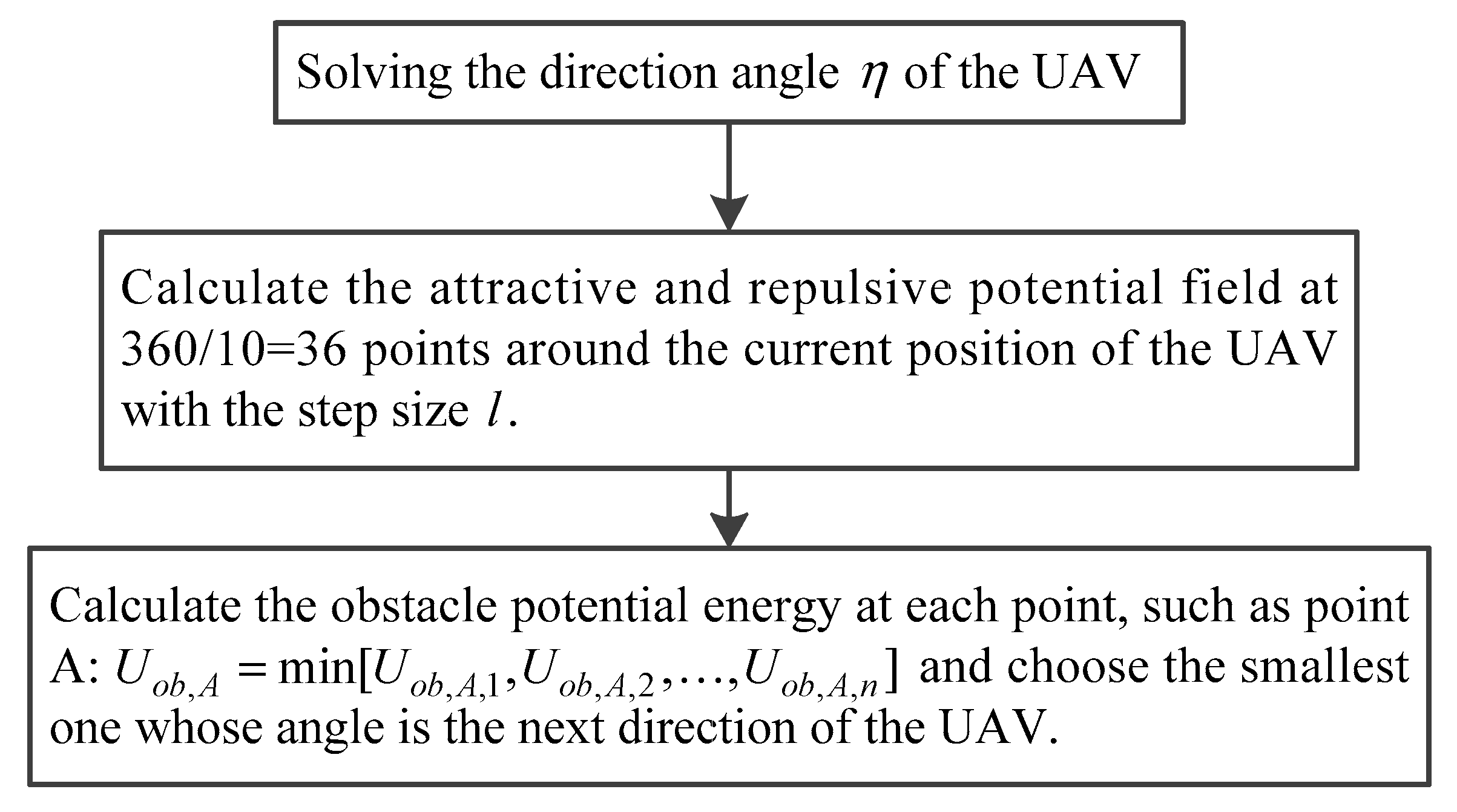
3.3. Path Optimization Based on Improved Artificial Potential Field Method

The equation of motion of the UAV during collision avoidance is:

$$\{\begin{array}{c}{P}_u(1,t+1)=P_u(1,t)+l\cos \eta \\ P_u(2,t+1)=P_u(2,t)+l\sin \eta \end{array}$$

(17)

$P_u(1,t+1)$ and $P_u(1,t)$ represents the position of the $x$ axis coordinates of the UAV at the moment $t+1$ and time $t$. $P_u(2,t+1)$ and $P_u(2,t)$ represent the $y$ axis coordinate position of the UAV at time $t+1$ and time $t$. $l$ is the step size of the UAV every moment, $\eta$ is the direction angle of the next moment of the UAV.

The gravitational potential field function is the same as the traditional artificial potential field method, and the potential field is expressed as $U_a={\zeta }_a{(P_{goal}-P_{UAV})}^2$. The repulsion potential field function uses a repulsion function of a Gaussian-like function [1]:

$$U_{rep,i}={\zeta }_{rep}\exp (-\frac{1}{{\sigma }^2}[{(x_u-x_{ob,i})}^2+{(y_u-y_{ob,i})}^2-r_u^2-r_{ob}^2])$$

(18)

where $x_u$ and $y_u$ represents the coordinate position of the current UAV, $x_{ob,i}$ and $y_{ob,i}$ represents the coordinate position of the obstacle $i$, $\sigma$ represents the standard deviation of the obstacle potential field, ${\zeta }_{rep}$ represents the range coefficient of the obstacle potential field, $r_u^{}$ indicating the size of the UAV, $r_{ob}^{}$ indicates the size of the obstacle.

It can be concluded that the entire potential field is: $U_t=U_a+{\displaystyle \sum U_{rep,i}}$. Assume that the total potential field in each direction at a certain point is $U_{t,1},U_{t,2},\dots ,U_{t,n}$. Take the direction of the smallest potential field as the direction of motion of UAV in the next times’ step. In order to make the UAV not shake in the collision avoidance process, the paper adopts a smooth strategy, that is, the potential field under the previous simulation step and the currently calculated potential field are summed according to a certain ratio, so that the direction will not become too fast and cause jitter. The potential field method concept map is shown in Figure 2 while the collision avoidance direction selection algorithm is shown in Figure 3.

3.4. UAV Formation Keeps Cluster Collision Avoidance Method

In this paper, two aspects are considered for the collision avoidance of the UAV cluster. One is that the UAV keeps the formation through the static obstacles, and the other is the collision avoidance between the two UAV groups that maintain the formation. The UAV formation flying collision avoidance method based on consensus algorithm are shown in Figure 4.

4. Simulation Case

For UAV formation collision avoidance, two practical scenarios should be considered when verifying the collision avoidance effect. The first is that when the obstacle is stationary, the UAV group can avoid the obstacle while maintaining the formation; the second case is that when the obstacle is also dynamic, the UAV group keeps the formation flight while avoiding the collision. To verify these two scenarios, we designed two classic scenes. One is a static obstacle scene, and the other scene is two UAV formations flying opposite with each other. These two scenarios are the most common and relatively difficult to solve. If the UAVs in the two scenarios successfully avoid collision, then the method is proved to be effective.

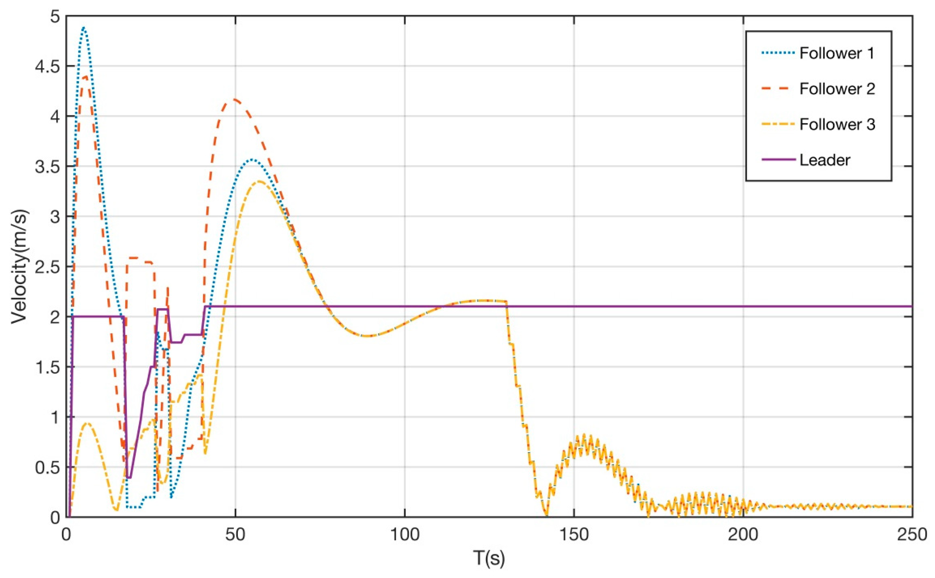
4.1. Static Obstacle Scene

In the experiment, each group of UAV consists of four UAVs, one of which is the leader UAV, whose target position, initial position and initial velocity were set in advance, followed by follower UAVs. The target position was set to (200, 200). The initial position and initial velocity of the follower UAVs were also set in advance. The initial positions of the four UAVs are shown in

Table 1. Static obstacle scene UAV initial position.

UAV	Initial Position (m, m)	Initial Velocity (m/s, m/s)
Follower 1	(0, 0)	(5, 0)
Follower 2	(60, 5)	(0, 3)
Follower 3	(30, 50)	(2, 2)
Leader	(20, 20)	(1, 1)

:

Figure 5 records the actual motion trajectories of the four UAVs, each of which took maneuvering measures to avoid collisions when encountering obstacles. In the initial formation of the formation, the UAV group formed a formation according to the consensus algorithm. When the obstacles were encountered, the UAVs in the UAV group performed the movement operation according to the improved artificial potential field method, then re-formed the formation. After the leader UAV reached the target position, the remaining follower UAVs slowed down and hovered in formation.

Figure 6. shows the relative distance between each pair of UAVs in the UAV group over time. From the curve in the figure, it can be seen that there is no collision between the UAVs, and the distance between the UAVs gradually stabilizes with the passage of time after passing through the obstacles, indicating that the UAV has formed a stable formation without the leader. After the UAV reached the target point, the follower UAVs shook back and forth nearby and slowly stabilized into a formation. When the leader UAV arrived at the target position, the follower UAVs continued to fly forward due to inertia, while the leader UAV slowed down, so the relative position between the leader UAV and follower UAVs suddenly became smaller, as shown in Figure 6.

Figure 7 shows the position of the UAV relative to the obstacle as a function of time. It can be seen from the enlarged partial view of the figure that the UAV’s closest distance to the obstacle was 5 m, which proves that the obstacle was avoided and free of collision during the flight.

Figure 8 records the velocity versus time curve of each UAV during flight. It can also be seen from the velocity curve that the UAV group is divided into three phases during the flight. The first phase is gradually changed from the irregular initial state. Forming a formation, so in the early follower UAVs, they first accelerated and then decelerated to achieve formation. When the obstacles were encountered, each UAV moved according to the trajectory generated by the artificial potential field. After the successful collision avoidance, the UAV group decelerated to a stable velocity to form a formation. Finally the UAV group reached the target point and then gradually slowed to a velocity close to 0, indicating that the UAV was in a hovering state. The three curves gradually return to zero, and one maintained the original velocity. Therefore, this means that the velocity of the three UAVs gradually decreased to near zero, and only one UAV maintained the original velocity. This is because the UAV cluster flight is based on the leader–follower model, and the leader UAV’s target velocity was set, so the performance in the simulation was that the leader UAV will shake at the original velocity when arrived at the target position, while the other followers UAV gradually reduced the velocity and formed a formation. In summary, three UAV gradually stopped, and the leader UAV swayed at the original velocity.

4.2. Dynamic Obstacle Scene

In this experiment, there were two groups of UAVs. Each group of UAV consists of four UAVs. One of the UAVs is the lead UAV. The target position, initial position and initial velocity were set in advance. The initial position and initial velocity of the follower UAVs were also set in advance. The initial positions of the eight UAVs of the two groups of UAVs are shown in

Table 2. Dynamic obstacle scene UAV initial position.

Group	UAV	Initial Position (m, m)	Initial Velocity (m/s, m/s)
Group 1	Follower 1	(0, 0)	(5, 0)
	Follower 2	(10, 25)	(0, 3)
	Follower 3	(0, 50)	(2, 2)
	Leader	(20, 20)	(1, 1)
Group 2	Follower 1	(190, 180)	(−5, −5)
	Follower 2	(210, 155)	(−3, −3)
	Follower 3	(180, 200)	(−2, −2)
	Leader	(170, 170)	(−1, −1)

.

Figure 9 records the actual motion trajectories of eight UAVs. Each UAV takes maneuvering measures to avoid collisions when encountering the other UAV group. Similar to the static obstacle scene, the UAV group formed a formation according to the consensus algorithm during the initial formation process. When the other UAV group was encountered, each UAV performed the motion operation according to the improved artificial potential field method. After passing the other UAV group, the UAV group re-formed the formation. After the leader UAV reached the target position, the other followers slowed down and hovered according to the formation.

Figure 10 shows the position of the UAV relative to the other UAV group over time. As can be seen from the enlarged partial view, the closest distance between the two UAVs is 5 m. The successful collision avoidance of the UAV group was realized during the flight. In the figure, the solid line indicates the relative distance between different groups of UAVs, and the dashed line indicates the relative distance between the UAVs in the same group. The initial relative distance was less than 50 m, which was the relative distance between the unmanned aerial vehicles in the same group, and the relative distance between the unmanned aerial vehicles in different groups was greater than 50 m. It can be seen from the dotted line that the closest relative distance between the UAVs in the same group was also greater than 5 m.

Figure 11 records the velocity versus time curve of each UAV during flight. It can also be seen from the velocity curve that the UAV group was divided into three phases during the flight. The first phase was the UAV group gradually changing from the irregular initial state. The follower UAVs first accelerated and then slowed down to achieve a formation. The second stage was that each UAV moved in accordance with the trajectory generated by the artificial potential field when encountering the obstacles. The third stage was that after the successful collision avoidance, the UAV group had an acceleration process and decelerated to a stable velocity to form a formation. After finally reaching the target point, the UAV gradually slowed down to a velocity close to 0, indicating that the UAV was hovering. We can find that there were three UAVs with non-zero but near-zero velocity at the end of the flight, the root cause was that the leader UAV was swinging back and forth with the original velocity at the end position, as the leader will still have had the pre-programmed original velocity. The follower UAVs still followed the consensus algorithm to follow the leader UAV to maintain the formation when the leader UAV arrives at the target position, and the leader UAV still maintained the original velocity at the target position due to the pre-set velocity, so the follower UAVs were also slowed down but still oscillating at the target position. These three UAVs obtained a non-zero velocity at the end of the flight because the follower UAVs will swing back and forth with a certain velocity calculated by the consensus algorithm.

5. Conclusions

This paper studied the formation of collision avoidance methods for UAV groups. The UAV group needs to form formations and fly to the target point when it is safe, and can effectively avoid obstacles when encountering them. The collision avoidance of static obstacle scene and the dynamic obstacle avoidance scene are simulated respectively in this paper, and the simulation results are analyzed. It is worth noting that the method is essentially a centralized control method, that is, the calculation is performed by the same calculation unit and then the control instruction is sent to the lower unit. But if the computational processor is efficient enough and there is little delay in the information transfer process, the method can be a distributed algorithm. In this case, each UAV acts as a computing unit and performs computational processing on the received information to generate its own decisions. In order to achieve a real flight test, we will design a control framework. The overall control framework consists of two aspects: The first aspect is about decision calculate, the other aspect is information sharing. For the first aspect, we would use the computing unit of the leader UAV to calculate the next moment trajectory of follower UAVs, then the leader UAV will send the control signal to the follower UAVs. For the second aspect, we set all follower UAVs to send their own velocity and location information to the leader UAV. This framework will enable information sharing and real flight.

The conclusions are as follows: (1) The contribution of this research is to study the formation maintenance method of the UAV group based on the second-order consensus algorithm, which can control each UAV in the formation and has a significant effect in forming a stable formation. (2) The application of the improved artificial potential field method in the collision avoidance problem of UAV is studied. The smoothing strategy is adopted to make the collision avoidance trajectory smooth and suitable for practical engineering use. (3) The collision avoidance between the UAV groups was studied. The UAV groups completed the formation while avoiding collisions and quickly formed a stable formation after the collision avoidance operation.

The recommendations and future work are as follows: (1) Propose a collision-avoidance solution in more complicated situations while maintaining the formation of the UAV formation; (2) Study the method while considering the communication delay between the UAVs; (3) Consider the formation change of the UAV group.

References

1. Fax, J.A.; Murray, R.M. Information flow and cooperative control of vehicle formations. IEEE Trans. Autom. Control. 2003, 49, 1465–1476. [Google Scholar] [CrossRef]
2. Jadbabaie, A.; Lin, J.; Morse, A.S. Coordination of groups of mobile autonomous agents using nearest neighbor rules. IEEE Trans. Autom. Control. 2003, 48, 998–1001. [Google Scholar]
3. Lawton, J.; Beard, R.; Young, B. A decentralized approach to formation maneuvers. IEEE Trans. Robot. Autom. 2003, 19, 933–941. [Google Scholar] [CrossRef] [Green Version]
4. Leonard, N.E.; Ogren, P. Obstacle avoidance in formation. IEE Icra 2003, 2, 2492–2497. [Google Scholar]
5. Tang, J.; Piera, M.A.; Guasch, T. Coloured Petri net-based traffic collision avoidance system encounter model for the analysis of potential induced collision. Transp. Res. Part. C: Emerg. Technol. 2016, 67, 357–377. [Google Scholar] [CrossRef]
6. Tang, J.; Zhu, F.; Piera, M.A. A causal encounter model of traffic collision avoidance system operations for safety assessment and advisory optimization in high-density airspace. Transp. Res. Part. C: Emerg. Technol. 2018, 96, 347–365. [Google Scholar] [CrossRef]
7. Olfati-Saber, R.; Fax, J.A.; Murray, R.M. Consensus and cooperation in networked multi-agent systems. Proc. IEEE 2007, 95, 215–233. [Google Scholar] [CrossRef]
8. Chen, Y.Q.; Wang, Z. Formation control: A review and a new consideration. Intelligent Robots and Systems. In Proceedings of the 2005 IEEE/RSJ International Conference on Intelligent Robots and Systems, Edmonton, AB, Canada, 2–6 August 2005. [Google Scholar]
9. Cao, Y.; Yu, W.; Ren, W.; Chen, G. An overview of recent progress in the study of distributed multi- agent coordination. IEEE Trans. Ind. Inform. 2013, 9, 427–438. [Google Scholar] [CrossRef]
10. Ren, W.; Beard, R. Consensus seeking in multi-agent systems using dynamically changing interaction topologies. IEEE Trans. Autom. Control. 2005, 50, 655–661. [Google Scholar] [CrossRef]
11. Ren, W.; Beard, R. Consensus of information under dynamically changing interaction topologies. In Proceedings of the American Control Conference, Boston, MA, USA, 30 June–2 July 2004; pp. 4939–4944. [Google Scholar]
12. Olfati-Saber, R.; Murray, R. Agreement problems in networks with directed graphs and switching topology. In Proceedings of the IEEE Conference on Decision and Control, Maui, HI, USA, 9–12 December 2003; pp. 4126–4132. [Google Scholar]
13. Olfati-Saber, R.; Murray, R. Consensus protocols for networks of dynamic agents. In Proceedings of the American Control Conference, Denver, CO, USA, 4–6 June 2003; pp. 951–956. [Google Scholar]
14. Jun, T.; Yang, W. A causal model for safety assessment purposes in opening the low-altitude urban airspace of chinese pilot cities. J. Adv. Transp. 2018, 2018, 1–18. [Google Scholar]
15. Luongo, S.; Corraro, F.; Ciniglio, U.; Di Vito, V.; Moccia, A. A novel 3d analytical algorithm for autonomous collision avoidance considering cylindrical safety bubble. In Proceedings of the 2010 IEEE Aerospace Conference, Big Sky, MT, USA, 6–13 March 2010; pp. 1–13. [Google Scholar]
16. Park, J.W.; Oh, H.D.; Tahk, M.J. Uav collision avoidance based on geometric approach. In Proceedings of the 2008 SICE Annual Conference, Tokyo, Japan, 20–22 August 2008. [Google Scholar]
17. Chakravarthy, A.; Ghose, D. Obstacle avoidance in a dynamic environment: A collision cone approach. IEEE Trans. Syst. Man Cybern. Part A Syst. Hum. 1998, 28, 562–574. [Google Scholar] [CrossRef]
18. Carbone, C.; Ciniglio, U.; Corraro, F.; Luongo, S. A novel 3d geometric algorithm for aircraft autonomous collision avoidance. In Proceedings of the 45th IEEE Conference on Decision and Control, San Diego, CA, USA, 13–15 December 2006; pp. 1580–1585. [Google Scholar]
19. Fasano, G.; Accardo, D.; Moccia, A.; Luongo, S.; Di Vito, V. In-flight performance analysis of a non-cooperative radar-based sense and avoid system. J. Proc. Inst. Mech. Eng. Part. G J. Aerosp. Eng. 2016, 230, 1592–1604. [Google Scholar] [CrossRef]
20. Orefice, M.; Vito, V.D.; Torrano, G. Sense and avoid: Systems and methods. In Encyclopedia of Aerospace Engineering; Wiley: New York, NY, USA, 2015. [Google Scholar]
21. Sigurd, K.; How, J. Uav trajectory design using total field collision avoidance. In Proceedings of the AIAA Guidance, Navigation, and Control Conference and Exhibit, Austin, TX, USA, 11–13 August 2003; p. 5728. [Google Scholar]
22. Liu, J.Y.; Guo, Z.Q.; Liu, S.Y. The simulation of the uav collision avoidance based on the artificial potential field method. Adv. Mater. Res. 2012, 591, 1400–1404. [Google Scholar] [CrossRef]
23. Ruchti, J.; Senkbeil, R.; Carroll, J.; Dickinson, J.; Holt, J.; Biaz, S. Unmanned aerial system collision avoidance using artificial potential fields. J. Aerosp. Inf. Syst. 2014, 11, 140–144. [Google Scholar] [CrossRef]
24. Yoshiaki, K. Real-Time Trajectory Design for Unmanned Aerial Vehicles Using Receding Horizontal Control; Massachusetts Institute of Technology: Cambridge, MA, USA, 2003. [Google Scholar]
25. Mavrovouniotis, M.; Yang, S.; Yao, X. Multi-colony ant algorithms for the dynamic travelling salesman problem. In Proceedings of the 2014 IEEE Symposium on Computational Intelligence in Dynamic and Uncertain Environments (CIDUE), Singapore, 16–19 April 2014; pp. 9–16. [Google Scholar]
26. Kim, D.H.; Shin, S. Local path planning using a new artificial potential function composition and its analytical design guidelines. Adv. Robot. 2005, 20, 115–135. [Google Scholar] [CrossRef]
27. Vascak, J. Navigation of Mobile Robots Using Potential Fields and Computational Intelligence Means. Acta Polytech. Hung. 2007, 4, 63–74. [Google Scholar]
28. McIntyre, D.; Naeem, W.; Xu, X.D. Cooperative Obstacle Avoidance using Bidirectional Artificial Potential Fields. In Proceedings of the 11th UKACC Control, Belfast, UK, 31 August–2 September 2016; pp. 1–6. [Google Scholar]
29. Chen, Y.B.; Luo, G.C.; Mei, Y.S.; Yu, J.Q.; Su, X.L. UAV trajectory planning using artificial potential field method updated by optimized control theory. Int. J. Syst. Sci. 2014, 45, 1407–1420. [Google Scholar]
Figure 1. Example of a simple graph.
Symmetry 11 01162 g001
Figure 2. Artificial potential field method concept map.
Symmetry 11 01162 g002
Figure 3. Collision avoidance direction selection algorithm based on artificial potential field method.
Symmetry 11 01162 g003
Figure 4. Unmanned aerial vehicle (UAV) formation flying collision avoidance method based on consensus algorithm.
Symmetry 11 01162 g004
Figure 5. UAV formation flight collision avoidance diagram in static obstacle scene.
Symmetry 11 01162 g005
Figure 6. Relative position map between UAV formation crews under the static obstacle scene.
Symmetry 11 01162 g006
Figure 7. Relative distance diagram of drone and obstacle in the static obstacle scene.
Symmetry 11 01162 g007
Figure 8. UAV velocity change diagram in the static obstacle scene.
Symmetry 11 01162 g008
Figure 9. UAV formation flight anti-collision diagram in dynamic obstacle scene.
Symmetry 11 01162 g009
Figure 10. Relative distance diagram of UAV and obstacle in dynamic obstacle scene.
Symmetry 11 01162 g010
Figure 11. UAV velocity change graph in dynamic obstacle scene.
Symmetry 11 01162 g011