Article

Hybrid Multi-Domain Analytical and Data-Driven Modeling for Feed Systems in Machine Tools

1
School of Mechanical Science and Engineering, Huazhong University of Science and Technology, Wuhan 430074, China
2
Department of EECS, Syracuse University, Snow City, NY 13244, USA
*
Author to whom correspondence should be addressed.
Symmetry 2019, 11(9), 1156; https://doi.org/10.3390/sym11091156
Submission received: 8 July 2019 / Revised: 5 September 2019 / Accepted: 9 September 2019 / Published: 11 September 2019

Abstract

:
Position error-compensation control in the servo system of computerized numerical control (CNC) machine tools relies on accurate prediction of dynamic tracking errors of the machine tool feed system. In this paper, in order to accurately predict dynamic tracking errors, a hybrid modeling method is proposed and a dynamic model of the ball screw feed system is developed. Firstly, according to the law of conservation of energy, a complete multi-domain system analytical model of a ball screw feed system was established based on energy flow. In order to overcome the uncertainties of the analytical model, then the data-driven model based on the back propagation (BP) neural network was established and trained using experimental data. Finally, the data-driven model was coupled with the multi-domain analytical model and the hybrid model was developed. The model was verified by experiment at different velocities and the results show that the prediction accuracy of the hybrid model reaches high levels. The hybrid modeling method combines the advantages of analytical modeling and data-driven modeling methods, and can significantly improve the feed system’s modeling accuracy. The research results of this paper are of great significance to improve the compensation control accuracy of CNC machine tools.

1. Introduction

Feed systems are used to position the machine tool components carrying the cutting tool and workpiece to the desired location [1]. They are one of the most important subsystems of computer numerical controlled (CNC) machine tools, as their positioning accuracy and speed determine the quality and productivity of machine tools [2]. Feed drive systems are either powered by linear motors directly, or by rotary motors via a ball screw and nut. Among them, ball screw feed drive systems are widely used in CNC machine tools for their high stiffness, reliable operation and ability to mitigate the impact of inertial and cutting force variations [3,4]. Machining accuracy significantly depends on the tracking performance of the feed systems for a given trajectory. Therefore, the ball screw should exhibit good transient and steady tracking performance to meet the demands of high productivity and high precision of machine tools [5,6].
To improve the tracking accuracy of the ball screw feed system, position error compensation control is commonly used. If the tracking error can be estimated accurately in advance, the control problem of the feed system can be eased. Therefore, a model of the ball screw feed system that can accurately predicted tracking error is essential to improve tracking performance. There are many factors affecting the tracking performance of the feed system, such as nonlinear friction, backlash, vibration, elastic deformation, thermal deformation and so on. These factors have attracted much attention and extensive research, and numerous papers have been published. Various friction models were researched in [7,8,9,10,11], such as stick-slip, static friction, Stribeck effects, and so on. Three kinds of backlash models, which are the hysteresis model [12], dead zone model [13] and vibration-impact model [14], can be found in previous studies. Another issue is the vibration; vibrations caused by the resonance of the feed drive were discussed and suppressed by using either the simplified model [15] or the complex model [16]. Some other studies have concentrated on the elastic deformation [17,18] and thermal deformation [19] of the ball screw feed systems. Most studies have used lumped-parameters models to analyze the ball screw feed systems. In order to overcome the shortcomings of lumped-parameters models, the investigation of hybrid, distributed-lumped parameter modeling methods for ball screw feed drive systems was conducted in earlier studies [20,21,22]. Besides, the finite element method (FEM) is also a common approach to model the ball-screw system. In [23], the FEM model was integrated with the servo dynamics to evaluate the dynamics response of the transmission system. The studies mentioned above have made significant contributions to improving the performance of the ball screw feed systems, but the theoretical analysis of the dynamic tracking performance of ball screw is very complicated; the influencing factors are so many so that it is difficult to further improve the prediction accuracy of tracking error based on theoretical analysis. What’s more, most studies have mainly concentrated on the modeling of the mechanical part, the coupling effects between different domains have not been considered.
The feed systems consist of multi-domain subsystems such as the mechanical transmission subsystem, electrical subsystem, control subsystem, and so on. These subsystems belong to different disciplines and there are complex coupling relationship among them. The performance of the feed system depends not only on the performance of the subsystems in each domain, but also on the interaction between them. In fact, the tracking errors of the ball screw feed system are mainly composed of two parts: the error caused by the servo control subsystem and the error caused by the mechanical subsystem. Therefore, a multi-domain integrated system model is essential to accurately predict the tracking performance. Research on multi-domain integrated modeling of ball screw feed systems has been rare so far. Some integrated modeling methods for feed systems in machine tools have been proposed [24,25,26,27,28]. In the references, the multi-domain coupling characteristics of a feed system were taken into account, but the modeling efficiency was low and it was hard to achieve real seamless integration due to use of the modeling method based on signal flow. Some attempts have been made to use the non-causal modeling method based on Modelica to establish the model of feed system, but the model was not strictly in accordance with the actual system and the model was not validated by experiment [29,30,31]. The deficiencies of existing research into integrated modeling of a feed system are that the parameters of the integrated model are too many, so they are difficult to determine accurately, meaning the accuracy of the model is limited.
According to previous research, the feed system model is usually derived from expert domain knowledge (e.g., basic physical principles). This modeling approach is called analytical modeling, also known as knowledge-driven, physics-based, or mechanism modeling. However, for complicated multi-domain systems such as feed systems, it is often too complex to derive their analytical model and to fully capture their dynamics. Additionally, the parameters may be time-varying or unknown, which limit the feed system’s modeling accuracy. The feed system model can also be established by machine learning techniques, which is called the data-driven modeling method. Machine learning is one of today’s most rapidly growing technical fields [32]; there has been growing interest in applying machine learning to draw insights gained from the data in engineering [33]. Data-driven analytics techniques have been applied for prediction [34,35,36,37], detection and classification [38,39], forecasting [40], control [41,42], and many problems of specific interest. For example, Zhe Li et al. [34] proposed a data-driven method for backlash error predication through the deep belief network (DBN). John C. Ziegert et al. [37] used an artificial neural network (ANN) to predict tool point positioning error in machine tools. Ronay Ak et al. [38] proposed a prediction model based on a neural network for estimating the energy consumption of a milling machine, while Gaussian process (GP) has been used to develop the data-driven energy prediction model with uncertainty for a milling machine [36]. Jinkyoo Park et al. [42] have discussed the data-driven modeling methods that are based on Bayesian statistic inference and illustrate their potential applications for performance characterization, condition diagnostic and control optimization of machine tool systems, for which analytical modeling of such systems can be difficult. Data-driven models are widely used and have achieved good results, but do not have interpretability and expressiveness. They need training data, but the data can hardly cover all working conditions. So, the fully data-based models may suffer from inaccuracies as well when the working condition of the feed system varies in a large range. In order to overcome the shortcomings of purely data-driven modeling methods, a hybrid analytical and data-driven modeling method was proposed. Relatively little related literature has appeared so far. René Felix Reinhart et al. [43,44] have used the hybrid analytical and data-driven modeling method to establish the kinematics model for soft robots and the inverse dynamic model for rigid robots. The authors only consider the hybrid modeling of robots at the component level.
This paper argues that an analytical model of a feed system should be established as a whole, incorporating mechanical, electrical, control, and other subsystems. Considered at system level, this paper develops a hybrid multi-domain analytical and data-driven model for the ball screw feed system to predict the tracking error. According to the law of conservation of energy, based on energy flow and symmetry transformation, a complete multi-domain system analytical model of the ball screw feed system is established. In order to compensate for the uncertainty of the model structure and parameters, a data-driven model based on a neural network was coupled to the multi-domain analytical model in parallel. The modeling method can implement seamless integration of complex systems in multiple domains and improve modeling accuracy. The hybrid model of the ball screw feed system was validated by experiment results.
The remainder of the paper is organized as follows. Section 2 introduces the multi-domain analytical modeling process for the ball screw feed system. Section 3 introduces the data-driven model. Section 4 introduces the hybrid modeling method for the ball screw feed system. Section 5 introduces the experimental verification of the hybrid model. Section 6 summarizes the full text.

2. Multi-Domain Analytical Model of the Ball Screw Feed System

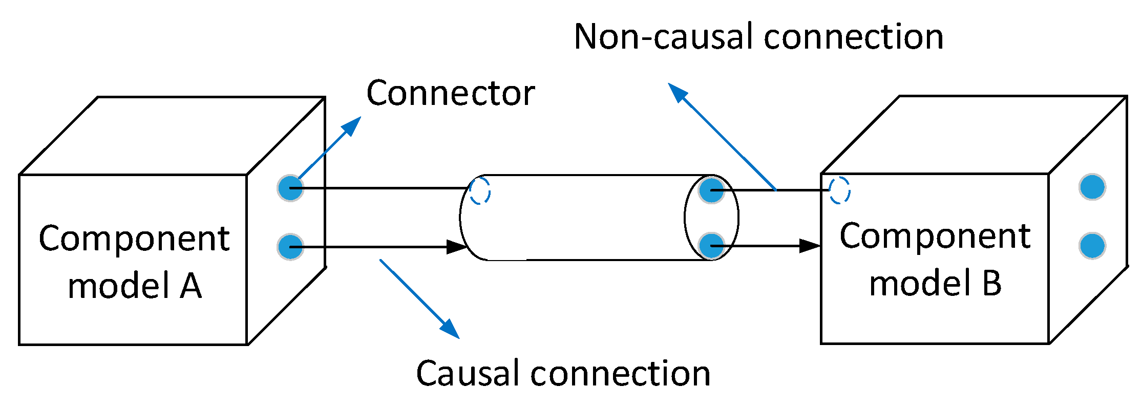
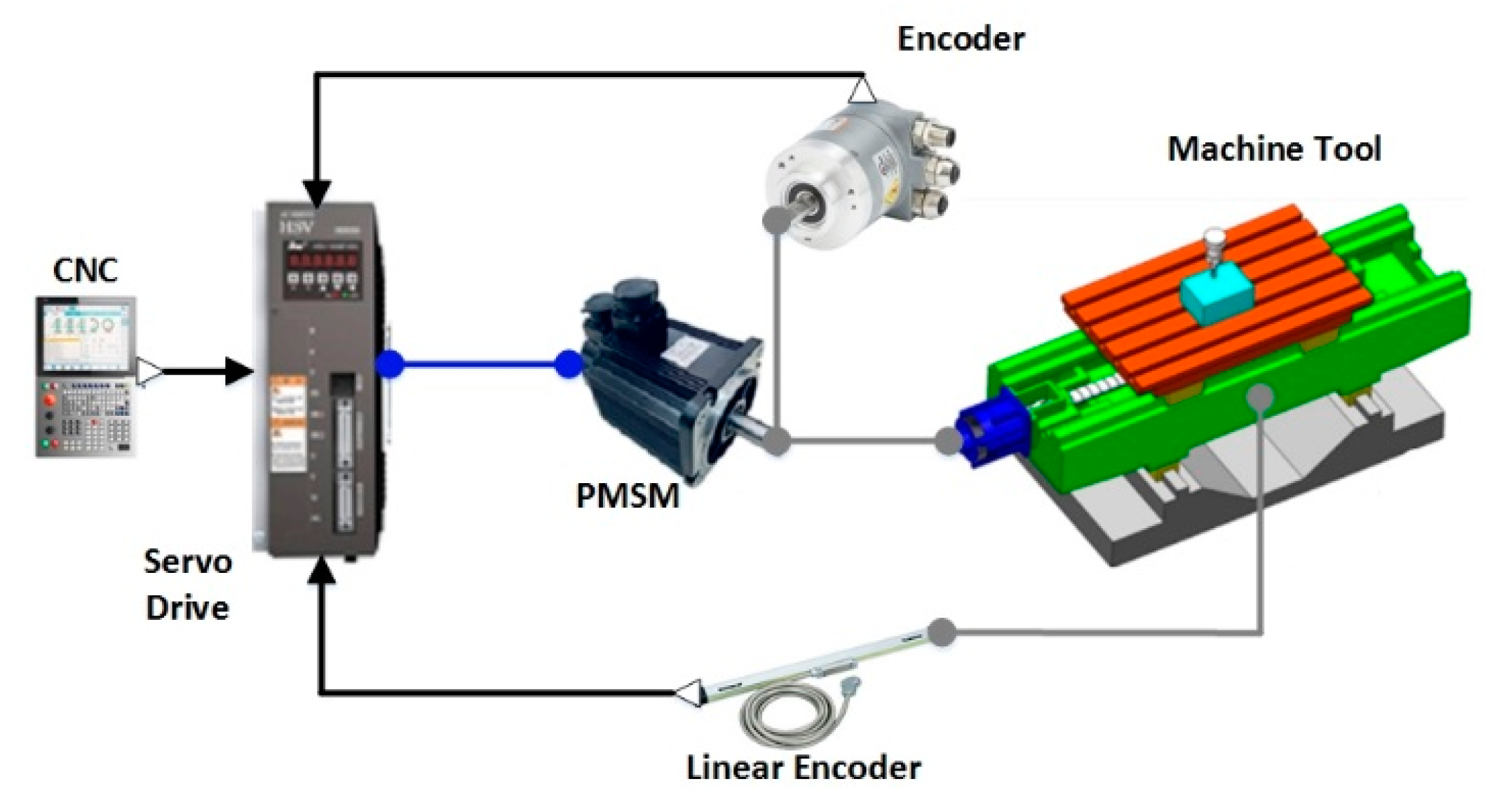
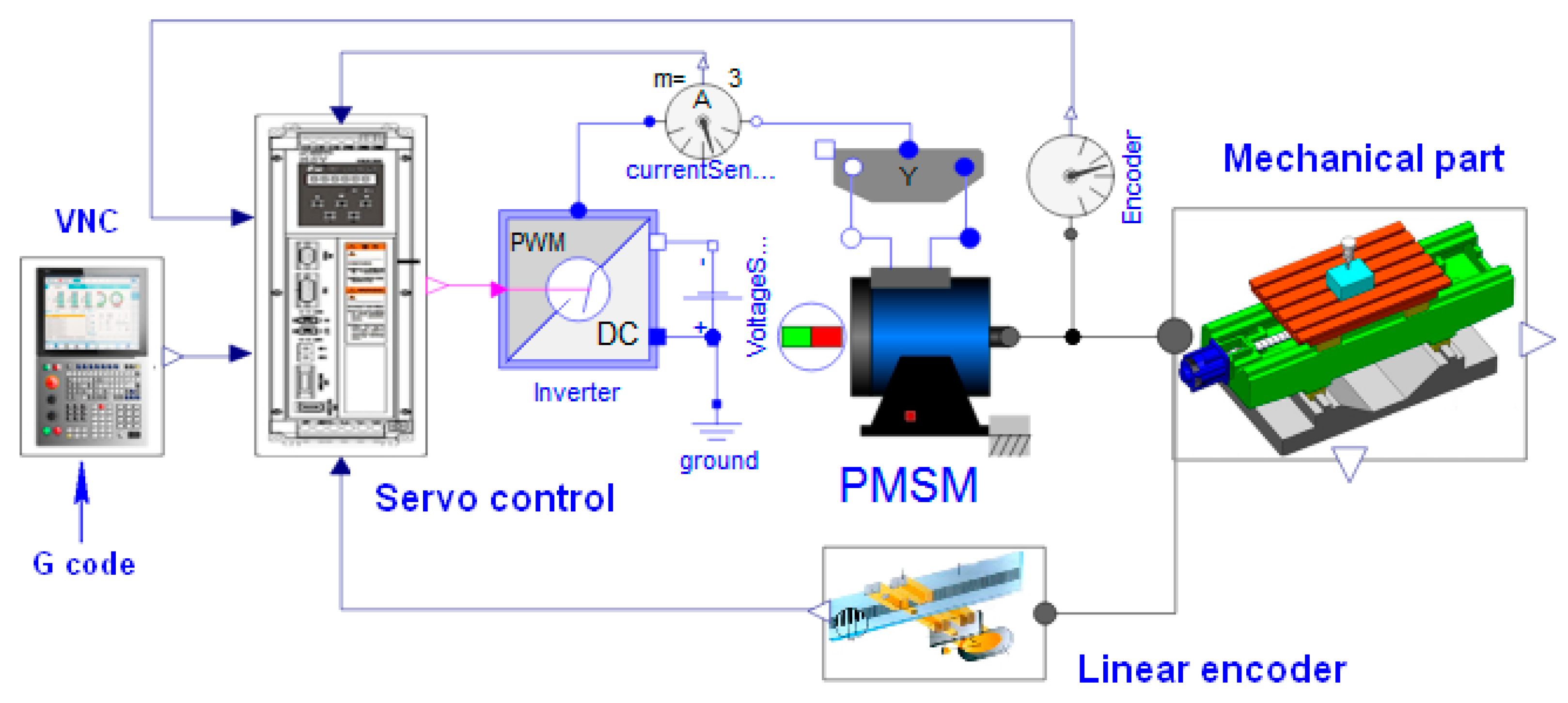
2.1. Multi-Domain Modeling Method for the Ball Screw Feed System

It is generally known that a ball screw feed system is a multi-domain integrated system which incorporates mechanical, control, electrical and other subsystems. This paper argues that the multi-domain coupling characteristics of the feed system should be taken into account when establishing an analytical model. Therefore, a modular non-causal modeling method based on Modelica language is used to establish the multi-domain analytical model of the feed system. Modelica is an object-oriented physical system modeling language, which supports the modeling of component models based on equations and the modeling of complex system based on component non-causal connection. In Modelica, the interface of the component model is called the connector, and the coupling relationship established on the component connector is called the connection. If the connection expresses a causal coupling relationship, it is called a causal connection. If the connection expresses a non-causal coupling relationship, it is called a non-causal connection. The component model connection mechanism is shown in Figure 1.
The key to establishing a multi-domain knowledge-driven model of ball screw feed system is how to divide the system and define the interfaces of component models in each domain. In this paper, the ball screw feed system is divided according to its real physical structure, then component models are established and its interfaces are defined, and finally the multi-domain integrated model of feed system is established by connecting component models. The ball screw feed system studied in this paper was driven by permanent magnet synchronous motor, and the module division of the system is shown in Figure 2. Each module can also be further divided into smaller modules.
In order that each component model can be connected, the uniform interface in each domain should be defined. In non-causal connection, the interface in each domain usually contains two types of variables: flow variables and potential variables. When the interface is connected, it satisfies the generalized Kirchhoff theorem, that is, the sum of flow variables is zero and the potential variables are equal. In causal connection, the connector includes input variables and output variables. In this paper, mainly the mechanical, control and electrical fields are considered, in which the connection in the mechanical and electrical fields is a non-causal connection, and the connection in the control field is a causal connection. The connectors defined are shown in Table 1:
The multi-domain analytical model of the ball screw feed system was developed base on Modelica language for its advantages and capabilities of component-based non-causal modeling. And the model mainly included the mechanical subsystem model, servo control subsystem model, the permanent magnet synchronous motor (PMSM) model, sensor models and other models. The structure of the model is shown in Figure 3.

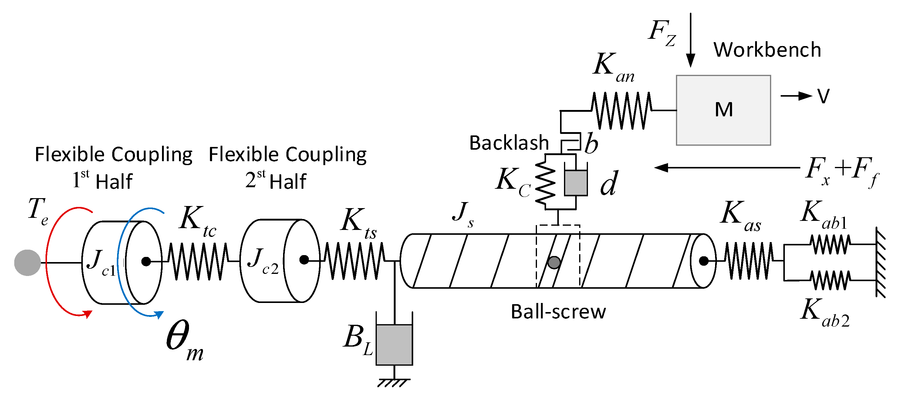
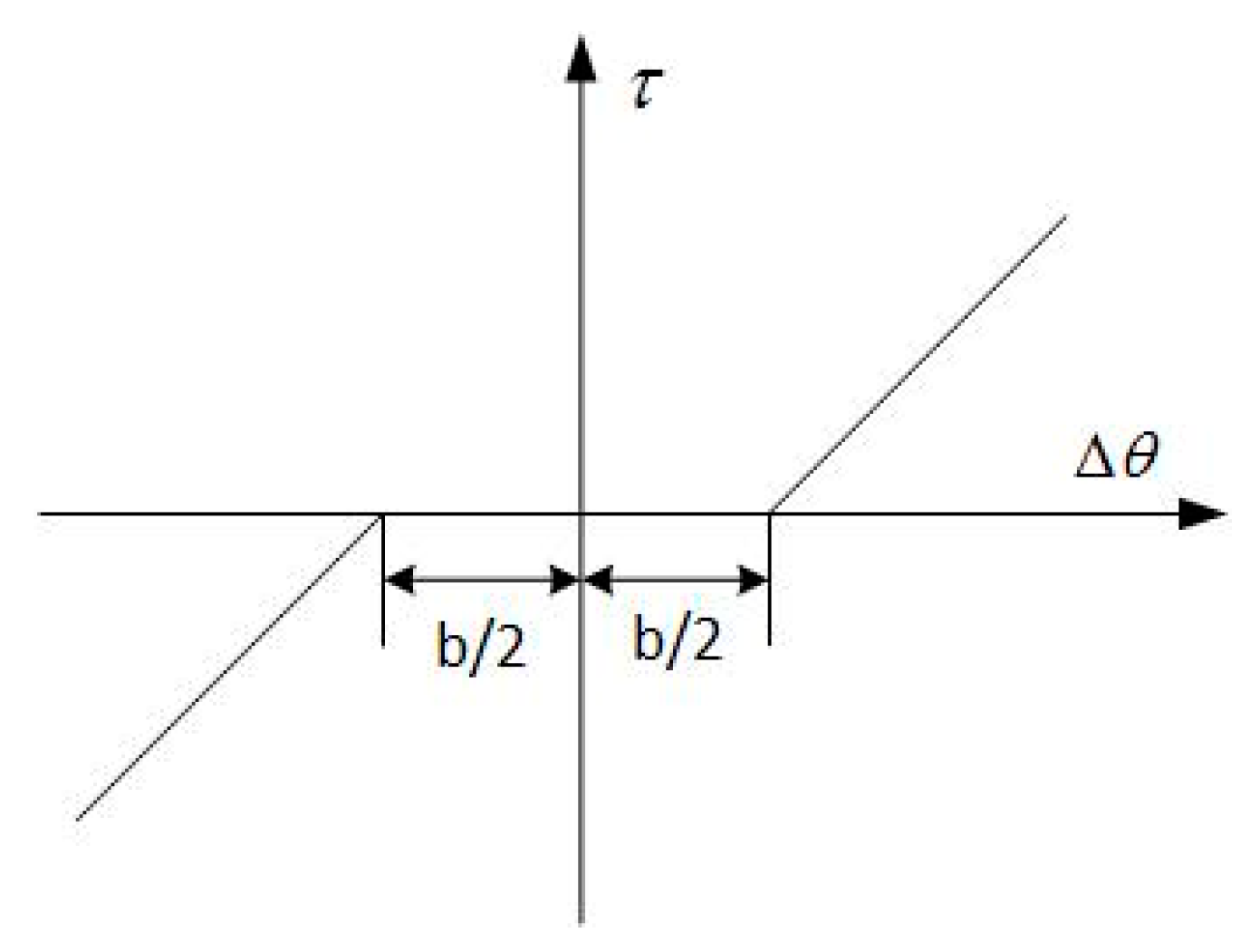
2.2. Modeling and Analysis of the Mechanical Subsystem

The mechanical part of a ball screw feed system is usually composed of sub-components, such as couplings, ball screws, supporting bearings at both ends, linear guide rails, screw nuts, the workbench, and so on. When establishing the mechanical subsystem model, the mechanical connector interface should be defined first, and then the component models are established based on the equation. The modeling schematic diagram is shown in Figure 4. The output torque of servo motors is represented as T e and the rotational and translational motion of mechanical parts are both driven by servo motors. The torsional stiffness of the coupling, the torsional stiffness and axial stiffness of the ball screw, the axial stiffness of the bearing and the screw nut, the backlash, and the nonlinear friction are all considered in the model.
For the servo motor, according to Euler’s law of motion, the torque balance equation on its output shaft is
T e = J m θ ¨ m + B m θ ˙ m + T L
where J m is the rotor inertia of the motor, θ m is the angular displacement of the output shaft of the motor, B m is the viscous damping coefficient and T L is the load torque on the motor shaft.
Considering the flexibility of each mechanical component, then
T L = K L ( Θ m Θ L )
where Θ L is the angular displacement of the screw shaft. K L is the total torsional stiffness converted from the stiffness of each component. K L can be calculated by the following equation, found in [27]:
1 K L = ( 2 π p ) 2 η 1 K Z + 1 K T
where K T is the total equivalent torsional stiffness of the feed system, K Z is the total equivalent axial tension compression stiffness of feed system, and η is efficiency of the driving mechanism. K T and K Z can be calculated as follows [27]:
1 K T = 1 K t c + 1 K t s
1 K Z = 1 K a s + 1 K a n + 1 K a b 1 + K a b 2
In the above equation, K t c is torsional stiffness of coupling, K t s is the torsional stiffness of the lead screw, K a s is the axial stiffness of the lead screw, K a n is the axial stiffness of the nut, K a b 1 and K a b 2 are the axial stiffness support bearing. The formulas for calculating the above stiffness parameters can be found in previous studies [10,27]:
K a s = E b s A s L s g x ( L s g x )
K a n = 0.8 K n 0 ( F p 0.1 C n 0 ) 1 3
where E b s is the elastic modulus of the lead screw material, A s is the sectional area of the lead screw, L s g is the distance between two supporting bearings, x is the distance between the nut and one end of the bearing, F p is the nut preload level, K n 0 is the contact stiffness of nut, and C n 0 is double nut pre-loading dynamic load rating.
For the lead screw, it is obvious that the moment balance equation on the shaft is
T L = ( J c + J s ) θ L ¨ + B L θ ˙ L + T t
where J c and J s are the moment of inertia of the coupling and the screw shaft respectively, T t is the load torque of the screw shaft.
There is backlash between the ball screw and the nut. The backlash has non-linear characteristics, which has a great influence on the positioning accuracy of the feed drive system. In this paper, a nonlinear elastic method [13] is used to establish the backlash model. The characteristics of the backlash are described by an abstract spring in the method. When the screw is in the gap zone, the spring stiffness is zero, and when the screw passes through the gap zone, the spring becomes stiff. The torque-angular displacement curve is shown in Figure 5.
For the ball screw feed system, when the backlash is considered, the load torque on the screw shaft can be calculated as follows:
T t = { K c ( Δ θ + b 2 ) + d Δ θ ˙               Δ θ < b 2   0                                 b 2 < Δ θ < b 2 K c ( Δ θ b 2 ) + d Δ θ ˙                 Δ θ > b 2    
In Equation (9), K c and d are the equivalent spring constant and equivalent damping of backlash respectively, b is the total backlash, and Δ θ = θ L θ t . θ t is related to the displacement of the workbench. Regardless of vibration, it can be seen in [18] that the displacement of the workbench S is:
S = ( p 2 π ) θ t S
S is the additional displacement of the worktable caused by the axial and torsional deformation of the lead screw, and
S = F K Z + ( p 2 π ) 2 1 η F K T
where F is the driving force of the workbench, which is generated by the torque T t ,
F = η 2 π p T t
For the workbench, according to Newton’s theorem, the force equilibrium equation is
F = M S ¨ + F x + F f
where F x is the axis component of cutting force. According to Stribeck model [10], the friction force F f can be calculated as follows:
F f = [ μ ( Mg + F z ) + μ v | S ˙ | + f s e b 0 S ˙ ] sgn ( S ˙ )
where the μ is the Coulomb friction coefficient, M is load mass, μ v viscous friction coefficient, f s is the Stribeck effect, b 0 represents the exponential decay.
By synthesizing the above formulas, the dynamic model of the mechanical part of the ball screw feed system can be established. The model is encapsulated and the interface for data exchange with other models is set up. The encapsulated model of the mechanical part can be seen in Figure 4.

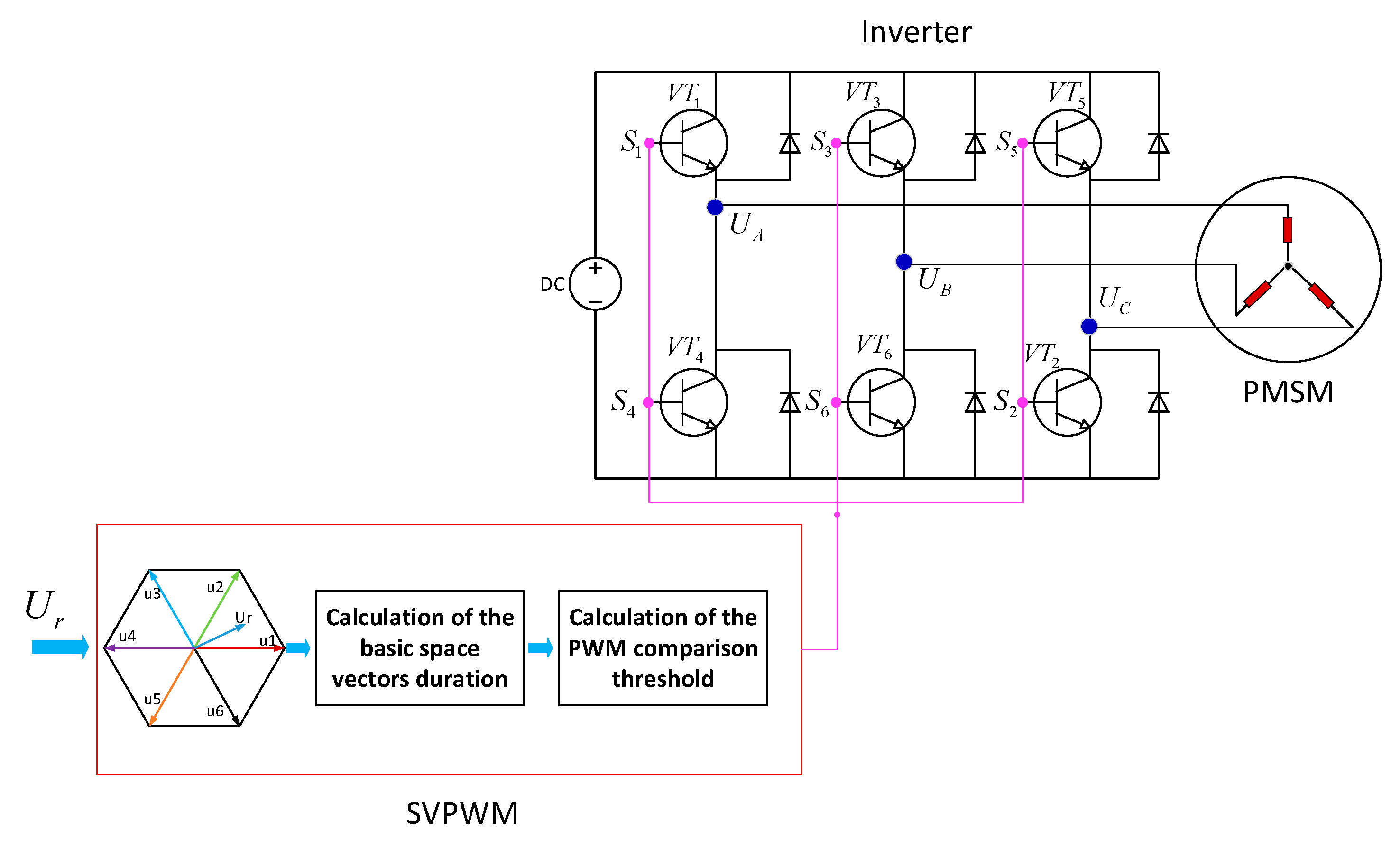
2.3. Modeling of the Servo Drive System

The feed system studied in this paper was powered by a permanent magnet synchronous motor, and the space vector control is used in servo drive system, which includes position control loop, speed control loop and current control loop. The motor was fed by a pulse width modulation (PWM) voltage source thyristor inverter, and the voltage modulation mode was space vector pulse width modulation (SVPWM) [45]. The servo drive system mainly included proportional integral (PI) controllers, coordinate transformation modules, the SVPWM module and inverter. In this paper, based on the analysis of the theory of space vector control, the modular modeling method described above is applied to establish the servo drive system model. First of all, the module models containing input and output interfaces are established.
Digital PI controllers are usually used in actual servo control systems. In order to keep the model consistent with reality, the model of digital PI controllers is established based on discrete control theory. The theory of digital PI control algorithm is as follows:
u ( k ) = k p e ( k ) + k p T i j = 0 k e ( j ) T
The coordinate transformation module includes Park transformation, Clark transformation and corresponding inverse transformation. These module models are established according to the transformation equation. The details of the Park and Clark transformation can be seen in [21].
The implementation of the SVPWM algorithm in vector control can be summarized as consisting of three steps: determination of the sector, calculation of the basic space vectors duration and calculation of the PWM comparison threshold, as shown in Figure 6.
According to the above analysis process, each module model was established based on the Modelica language, and then the SVPWM module model was obtained by connection. The outputs of the SVPWM model are the control signal of the inverter switch tube. The topology circuit of the inverter is shown in Figure 6: VT1~VT6 are power switch tubes, and the on-off of each switch is controlled by the drive signal S1~S6, U A , U B and U C is the output voltage of the inverter. In this paper, the electrical interface model, power switch transistor and diode model are established first, and then the inverter model is established by connecting the component models according to the topology circuit structure of the inverter. Similar to the model of mechanical parts, the servo control subsystem model was encapsulated and several interfaces set up, as shown in Figure 6.

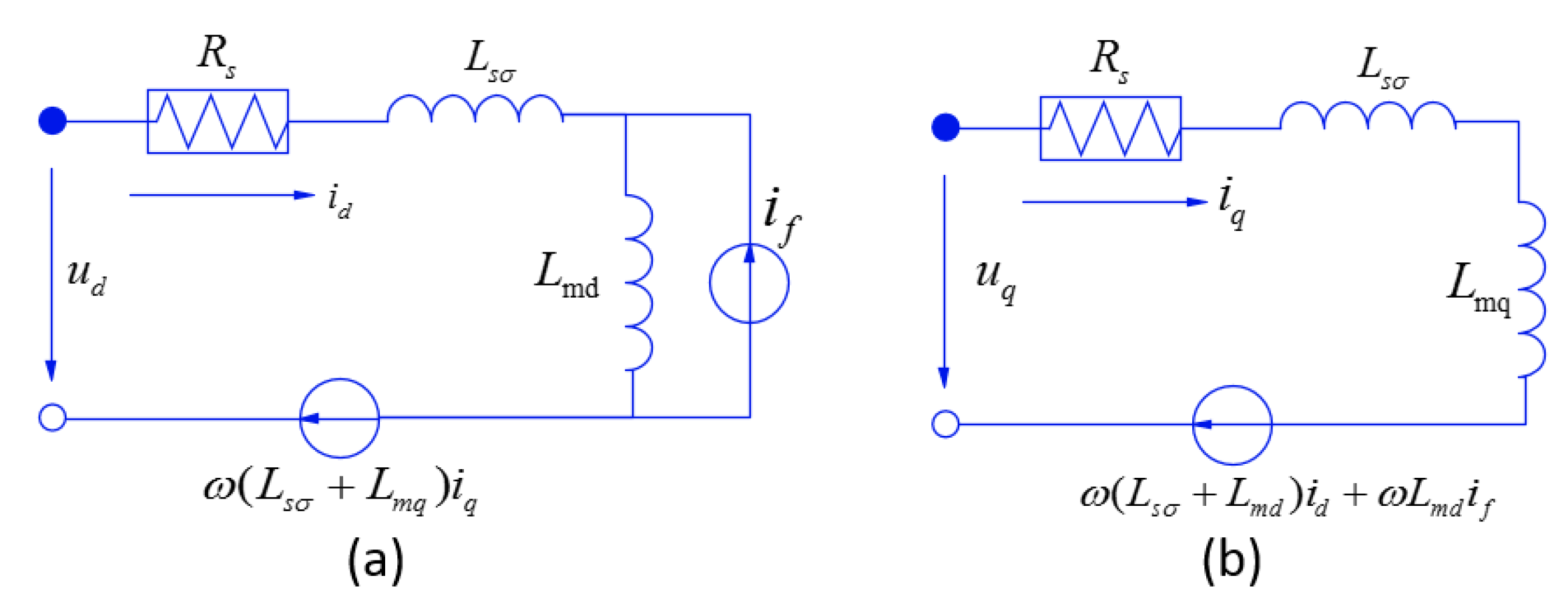
2.4. Modeling of the Permanent Magnet Synchronous Motor

The electromagnetic relations of the PMSM are very complicated. In order to simplify the analysis, some assumptions are made as follows:
(1)
The conductivity of permanent magnet material is zero;
(2)
There is no damping winding on the rotor;
(3)
Stator winding current produces only sine distribution of magnetic potential in the air gap, ignoring the high-order harmonic of magnetic field;
(4)
During the steady-state operation, the waveform of induction electromotive force in phase winding is sinusoidal.
The physical quantities of AC motor windings, such as voltage, current and flux, vary with time, and time phasors are often used to represent them in analysis. However, they can also be defined as spatial vectors if considering the space position of the windings. The synthetic vector formed by the same physical quantity in three-phase windings is the synthetic space vector of this physical quantity. The symmetrical three-phase current, voltage and flux linkage in three-phase symmetrical stator windings of permanent magnet synchronous motor can be regarded as the space vector. Through coordinate transformation of the space vector, the mathematical equation of permanent magnet synchronous motor in a two-phase rotating coordinate system can be derived [45].
The voltage equation of d and q axis is shown as follows:
u d = R s i d + d ψ d d t ω ψ q
u q = R s i q + d ψ q d t + ω ψ d
where ω is the electrical rotor angular speed, R s is equivalent stator resistance, u d and u q are the d -and-q-axis voltage, i d and i q are the d -and-q-axis current, ψ d and ψ q are the d -and-q-axis flux linkage.
The flux linkage equations of d and q axes are as follows:
ψ d = L s σ i d + L m d i d + L m d i f
ψ q = L s σ i q + L m q i q
where L s σ is the damper stray inductance, L m d is the stator main field inductance per phase in d-axis, L m q is stator main field inductance per phase in q-axis, i f is the equivalent excitation current of the rotor permanent magnet. i f is a parameter and the calculation of it can be seen in [46]. The electromagnetic moment equation acting on the motor shaft is as follows:
T e m = 3 2 p ( ψ d i q ψ q i d ) = 3 2 p L m d i f i q
where T e m is the electromagnetic torque and p is the number of pole pairs.
Based on the above PMSM mathematical model, the equivalent circuit of PMSM in d and q axis coordinates can be obtained, as shown in Figure 7:
Based on the analysis and the equivalent circuit mentioned above, and considering the loss models of copper, iron and friction, a permanent magnet synchronous motor model is established in this paper. The encapsulated model of the PMSM can be seen in Figure 7. Completely accurate PMSM modelling is difficult to obtain because that PMSM is a high-order, non-linear, strong coupling system. So, some assumptions have been made to analyze the PMSM model. The error produced by these assumptions is hard to avoid, but the error can be reduced by modifying the model parameters through experiments. What’s more, the error can be compensated for to a certain extent by the data-driven model.

3. The Learned Data-Driven Model

The accuracy of the analytical model can hardly reach a high level because the model can hardly capture all aspects of the feed system’s intrinsic properties, and there remain unmodeled dynamics. Therefore, a data-driven model was developed as a supplement to the analytical model.
In this thesis, the data-driven model was used to fit the deviation between the output of the analytical model and the measured value. A back propagation neural network (BPNN) was chosen to build the data-driven model because the data-driven model is small in scale and the BPNN structure is simple, the local extremum points are few, the fitting accuracy is high, and it is easy to transplant. The structure of BPNNs can be divided into input layer, hidden layer and output layer. In the hybrid model, the data-driven model was used to predict the deviation between theoretical model output and measured value. The scale of the data-driven model was relatively small, so a three-layer BPNN was chosen in which the position command signal and the working table displacement output from analytical model were the input layer neurons. There was only one output neuron which was the deviation between the working table displacement measured by experiment and that simulated by the analytical model. The relevant theory of BPNN can be referred to [47]. Combining with the empirical formula, the number of neurons in the hidden layer was determined by the trial and error method. The number of neurons in the hidden layer is 10 and the empirical formula is shown as follows
l < m + n + a
In Equation (21), m , n and l are the number of nodes in the input layer, output layer and hidden layer respectively, and a is a constant between 0 and 10.
BP neural network represents the mapping relationship between n independent variables and m dependent variables. Before making a prediction, network training is needed to give it the ability to perform association and decision-making. If ω i j represents the connection weights between input layer i and hidden layer j , v j k represents connection weights between hidden layer j and output layer k , a j and b k represent the thresholds of hidden layer j and output layer k , respectively, then the output of the hidden layer is:
H j = f 1 ( i = 1 n ω i j x i a j ) ,       j = 1 , 2 , , 10 , n = 2  
In Equation (22), f 1 is the activation function of the hidden layer. The sigmoid function shown in Equation (23) was chosen in this paper.
f 1 ( x ) = 1 1 + e x
The output of the BP network is shown as follows:
O k = f 2 ( j = 1 l H j v j k b k ) ,   k = 1 , l = 10
In Equation (24), f 2 is the activation function of the output layer and that the function f 2 ( x ) = x was chosen in this paper.
If Y 1 represents the actual value of the deviation between measured working table displacement and that simulated from the analytical model, then the error function of the BP network is shown as follows.
E = 1 2 ( Y 1 ( j = 1 10 ( f 1 ( i = 1 2 ω i j a j ) v j 1 b 1 ) ) ) 2
The weights and thresholds of the BPNN are updated by gradient descent method of error function.
In order to train the BPNN, some input and output label data are collected by experiment, as shown in Figure 8.
The input working table command displacement shown in Figure 8a is the sinusoidal signals with periods of 12 π seconds in the first 30 s and periods of 2 π seconds in the rest of the 30 s, and that the amplitude of the signal is 0.1 m. The second input of the BPNN shown in Figure 8b is the simulation working table displacement of the analytical model. The output label of the BPNN shown in Figure 8c is the deviation between measured working table displacement and that simulated from analytical model. Use of the steepest gradient descent method to train the BPNN data-driven model and the results are shown in Figure 9.
In Figure 9, the Loss is the variance of the deviation between the label value and the output of the BP network model. It can be seen that after about 2000 training sessions, the loss value tended to be stable. The data-driven model can be established by using the DBN [34], ANN [37], GP [36] and so on. In this paper, the simple BP network was chosen to avoid over-fitting because of the data-driven model is small in scale. After a great quantity of training, the weights and thresholds of the data-driven model can be learned.

4. Hybrid Model of the Ball Screw Feed System

The multi-domain hybrid modeling method proposed in this paper combines the advantages of analytical and data-driven modeling methods. The principle of this hybrid modeling method is shown in Figure 10.
The hybrid model consists of two parts, which are the multi-domain analytical model and data-driven model. The model can be expressed by the following mathematical formula.
y ^ = f ( x , p ) = f k ( x , p k ) f d ( x , p d )
In the formula, x R m and y ^ R n are input and output vectors, f is a function for the hybrid model relation between x and y ^ , and f k and f d are the functions associated with analytical model and data-driven model. p R p is the parameter vector of the function f , and p k and p d are the parameter vectors associated with the function f k and f d , respectively. The symbol “ ” represents a coupling operation between the analytical model and data-driven model. Based on experimental and simulation data and parameter identification algorithm, the parameters p k can be identified. The parameters p d can be obtained by the training algorithm.
In general, a model that can learn from data without using any domain knowledge is called a data-driven model, for example, artificial neural networks, support vector machines, fuzzy methods, generalized linear models, and so on. In this thesis, the data-driven model is used to fit the deviation between the output of the analytical model and the measured value. The mathematical expressions of the coupling between knowledge-driven model and the data-driven model are given by the following:
y ^ = f ( x , p ) = f k ( x , p k ) + f d ( x , f k ( x , p k ) , p d )
The data-driven model can be learned after training and then the data-driven model is coupled with the analytical model and the hybrid model of the ball screw feed system is established as shown in Figure 11.

5. Simulation and Experiments

In order to validate the multi-domain hybrid system model, a ball screw feed system test platform was set up as shown in Figure 12. The position command signal of the working table was generated by the numerical control device. The angular displacement of the servo motor could be measured by the photoelectric encoder and the position of the workbench could be measured by the linear encoder. Given the different types of position command signals, the actual position, velocity and acceleration of the working table, and the output torque of the servo motor, and so on, could be measured by the corresponding experimental instruments.
The main parameters of the ball screw feed system are listed in Table 2. When these parameters were imported into the multi-domain hybrid model of feed system, the tracking error could be predicted by the model and the comparison between the measured results and the simulation results could be performed.

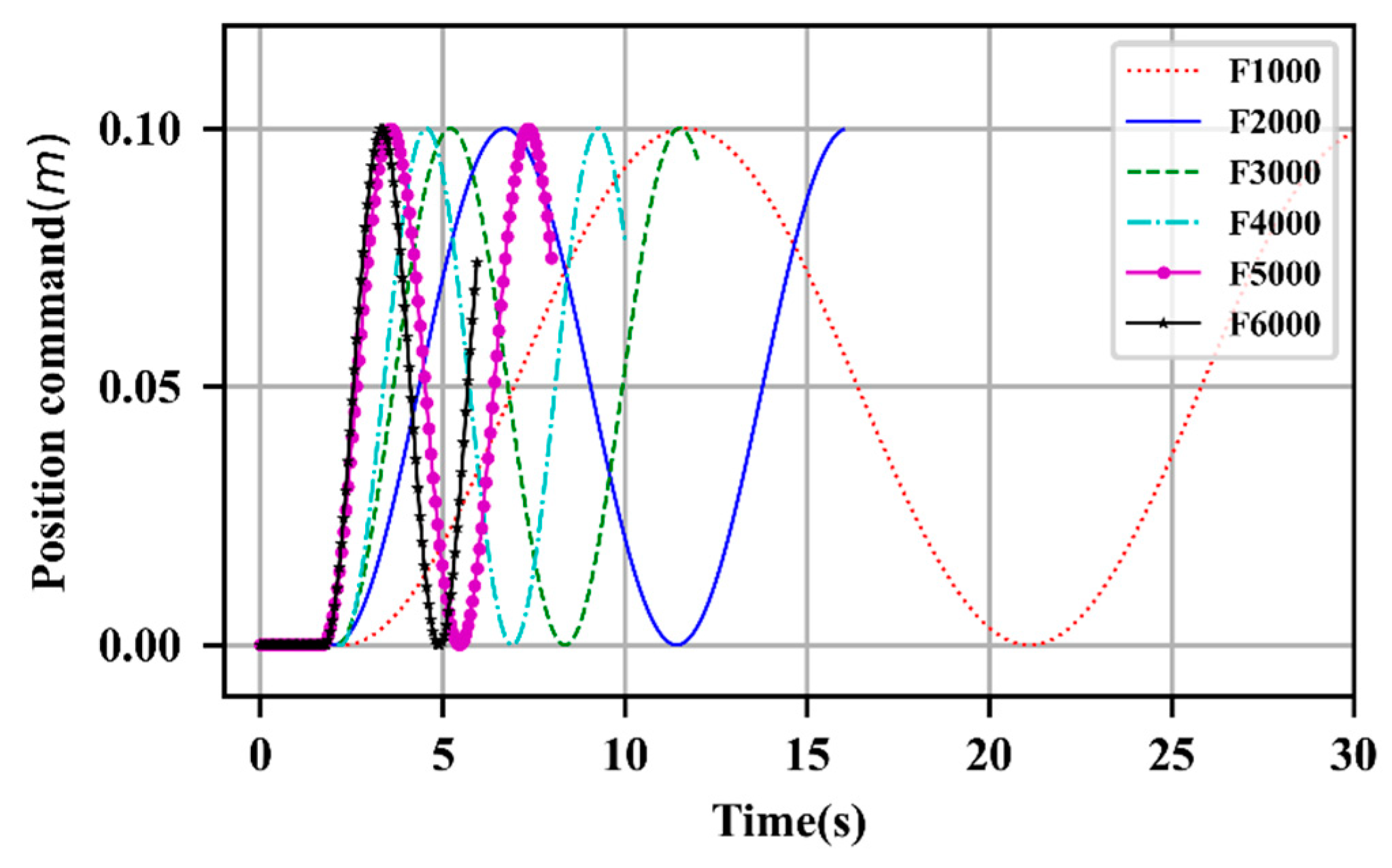
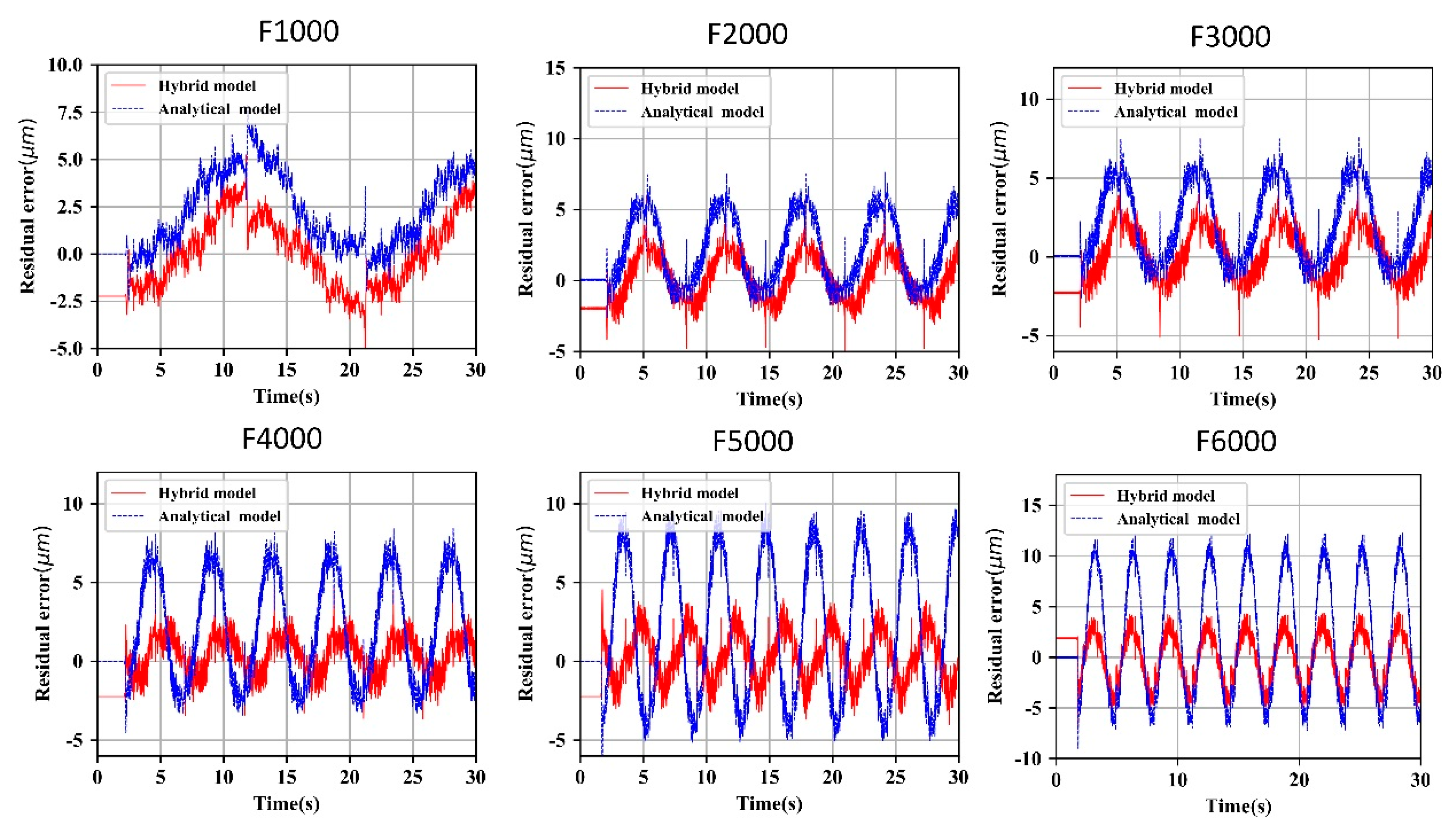
5.1. Single Axis Ball Screw Feed System Hybrid Model

First, the single-axis ball screw feed system hybrid model was verified under the sinusoidal position command signal (the given position command signal varies with time according to the sinusoidal law). The G code was loaded to make the displacement of the working table change with time according to sinusoidal law. The maximum feed speed was set to 1000 mm/min, 2000 mm/min, 3000 mm/min, 4000 mm/min, 5000 mm/min, and 6000 mm/min respectively, and the stroke was set to 100 mm. The given position command signals of the working table are shown in Figure 13.
The sinusoidal position command signal with the maximum feed speed of 1000 mm/min and 6000 mm/min were used to train the data-driven model, and the rest of the signals were used to verify the hybrid model. The same G code was imported into the hybrid model and then the simulation results were compared with the measured results.
If S m represents the displacement of the workbench measured by the experiment, S A p represents the displacement predicted by the pure analytical model, S H p represents the displacement predicted by the hybrid model, and S is the command displacement, then the dynamic tracking errors can be defined as follows:
{ E m = S m S E A p = S A p S E H p = S H p S
where E m is the tracking error measured by the experiment, E A p is the tracking error predicted by the pure analytical model and E H p is the tracking error predicted by the hybrid model. The hybrid model prediction error ( E H p E m ) and the analytical model prediction error ( E A p E m ) were compared, as shown in Figure 14.
It can be clearly seen in Table 3 that the prediction accuracy of the hybrid model was higher than that of the pure analytical model. To evaluate the difference between the simulation results and experiment results quantitatively, the maximum absolute error (MAE), root mean square error (RMSE) and relative error (RE, refers to the ratio of absolute error to measured true value, expressed as percentage) were evaluated. The simulation accuracy of the hybrid model and the analytical model can be seen in Table 3. The results show that the maximum deviation of the tracking error between the measured and predicted by the hybrid model were all under 6.79 μm. The RMSE of the prediction errors were all under 2.63 μm and the RE decreased gradually as the feed rate increased. The comparison of results showed that, compared with the pure analytical model, the hybrid model can improve the accuracy of tracking error prediction, and the accuracy of the hybrid model proposed in this paper can reach a relatively high level.

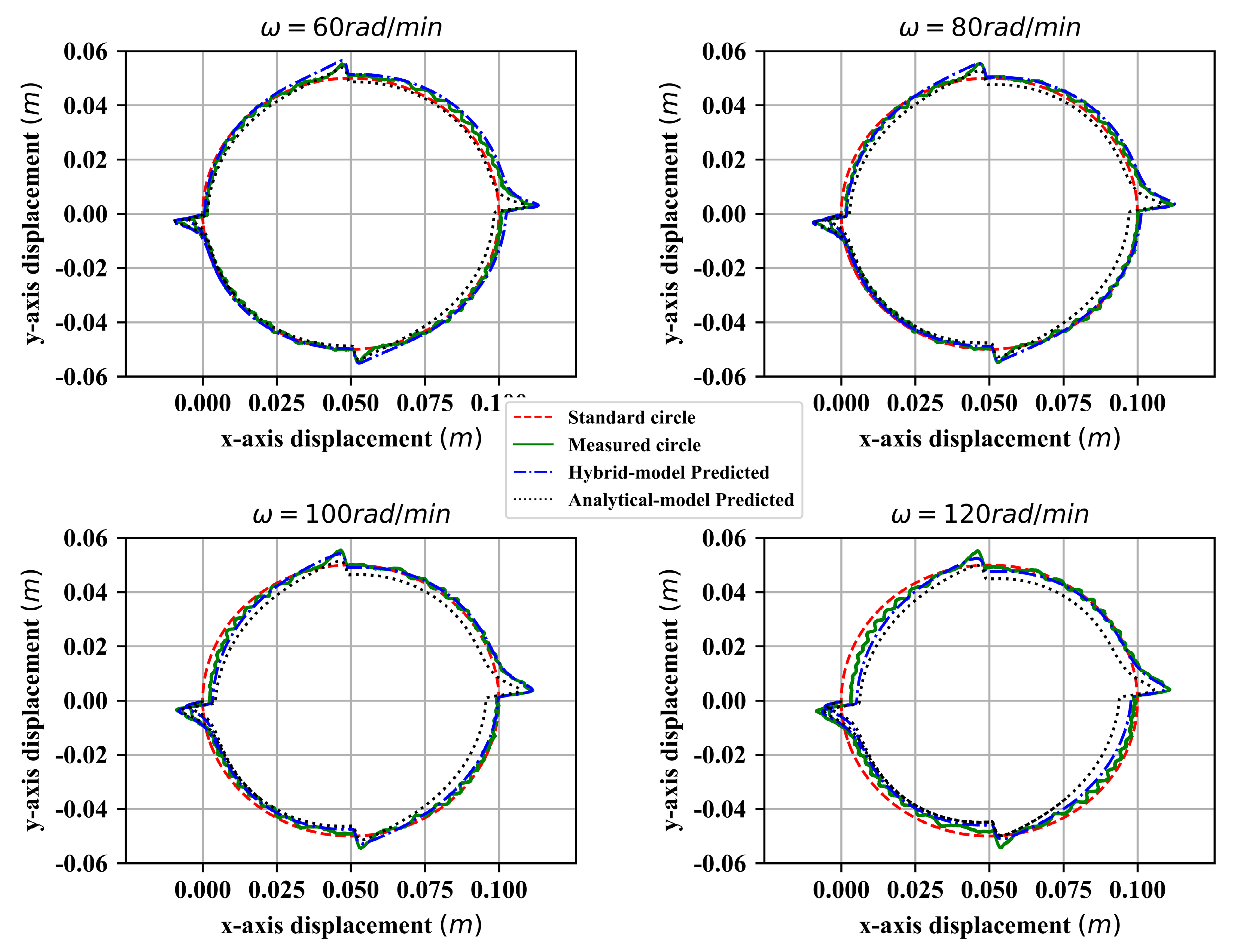
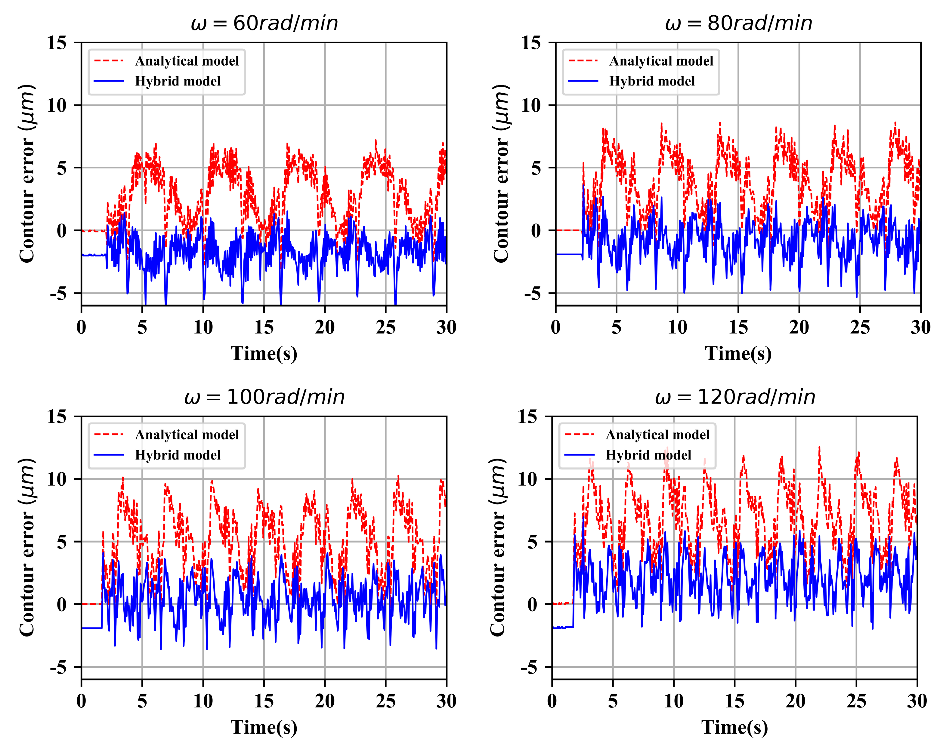
5.2. Double Axis Ball Screw Feed System Hybrid Model

The double axis ball screw feed system consisted of the x-axis feeding system and the y-axis feeding system. The system model was established with the use of the hybrid multi-domain analytical and data-driven modeling method proposed in this paper, and it can be used to predict contour error. The accuracy of the model was verified by experiment under different speeds of circle drawing. The experimental velocities included 60 rad/min, 80 rad/min, 100 rad/min and 120 rad/min. The simulation and experiment results are shown in Figure 15. (The circle contour error is magnified 500 times in the figure).
There are four circles in Figure 15, they are the standard circle, experiment circle, analytical model-predicted circle and the hybrid model-predicted circle. The standard circle is the trajectory command given by the numerical control device and the experiment circle is the trajectory measured by the linear encoder. The predicted circles of the pure analytical and the hybrid model are compared in the figure. As can be seen in the figure, the circle predicted by the hybrid model was much closer to the experimental circle than the circle predicted by the pure analytical model. Especially at high speed, the advantage of the hybrid model was more obvious. As the angular velocity increased, the prediction effect of the pure analytical model was getting worse. The contour error curves predicted by the pure analytical model and the hybrid model are show in Figure 16. It can be seen in the figure that the contour error predicted by the hybrid model was much smaller than that the analytical model predicted. Also, the contour error predicted by the analytical model increased as the angular velocity increased, whereas the contour error predicted by the hybrid model did not change much.
Comparison of the maximum contour error predicted by the hybrid model and the pure analytical model are shown in Table 4. The results show that the maximum contour error predicted by the hybrid model can reach 6.96 μm and the prediction ability is better than the pure analytical model.

6. Conclusions

This paper proposed a multi-domain hybrid analytical and data-driven modeling method for the ball screw feed system in machine tools, and a hybrid model of a single-axis and double-axis ball screw feed system were developed by the proposed modeling method. The hybrid model comprised an approximate multi-domain analytical model and a learned, data-driven error model. Experiments were performed to validate the accuracy of the hybrid model and the results show that the model can significantly improve the feed system’s modeling accuracy. The main conclusions of this article are as follows:
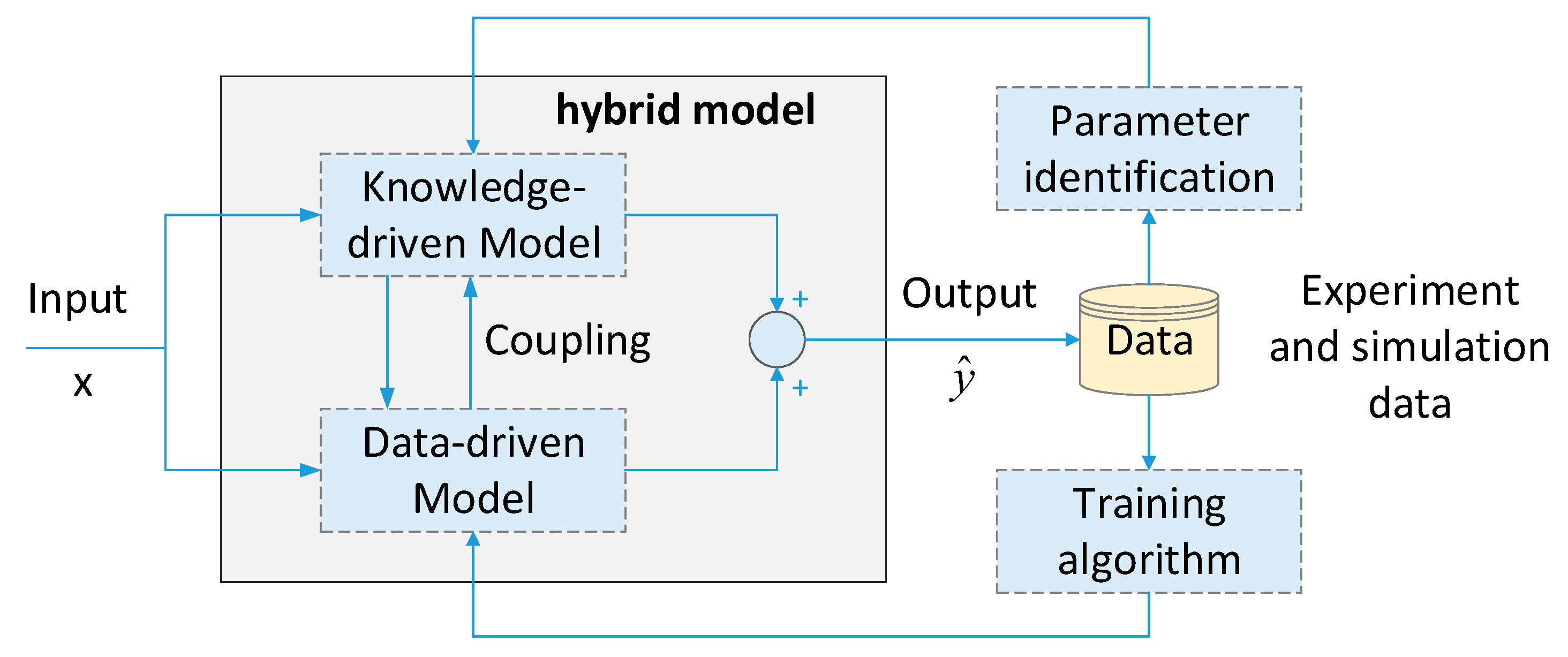
  • A hybrid multi-domain analytical and data-driven modeling method was proposed in this paper and a hybrid model of a ball screw feed drive system was established accurately using the hybrid modeling method.
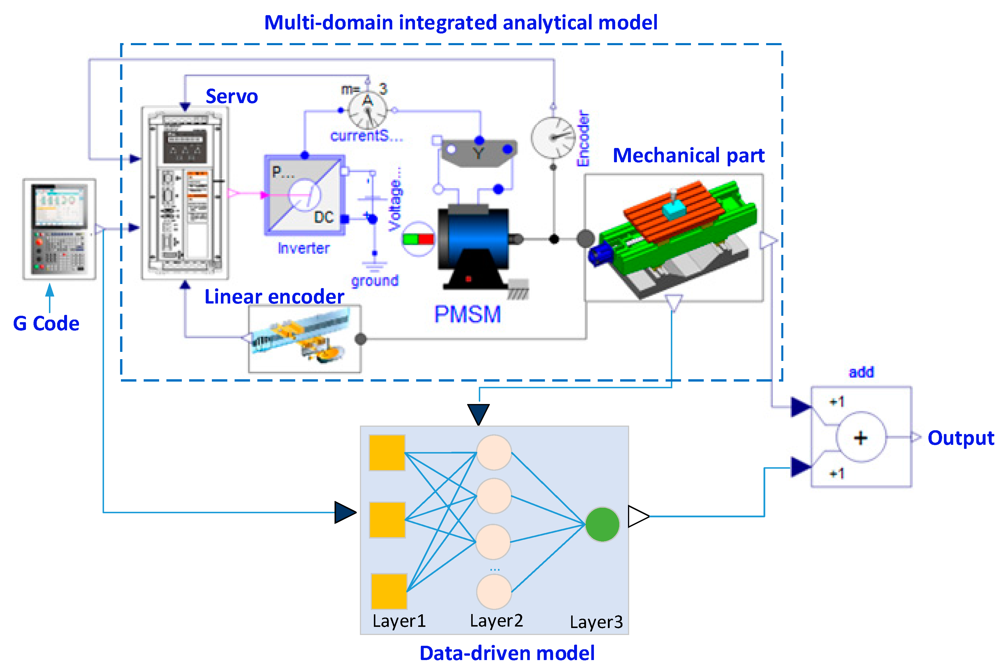
  • In contrast to the traditional causal modeling method based on signal flow, the multi-domain integrated analytical model of the ball screw feed system was established using the non-causal modeling method based on energy flow. The analytical model of a feed system developed in this paper realized seamless integrated modeling of a complicated multi-domain system.
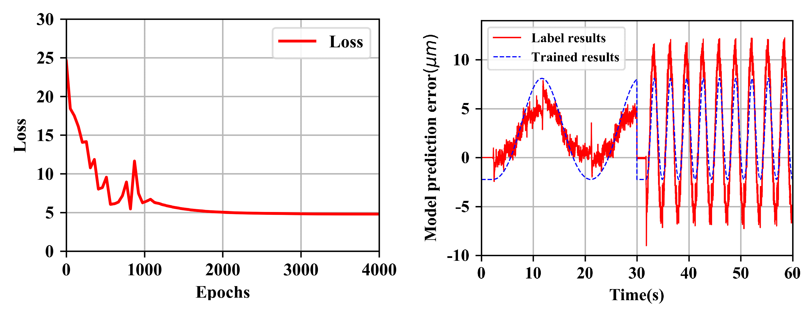
  • A data-driven error model based on a BP neural network was established and the model was trained using experimental data. Then the learned data-driven error model was coupled with the analytical model of the ball screw feed system and the hybrid model was obtained.
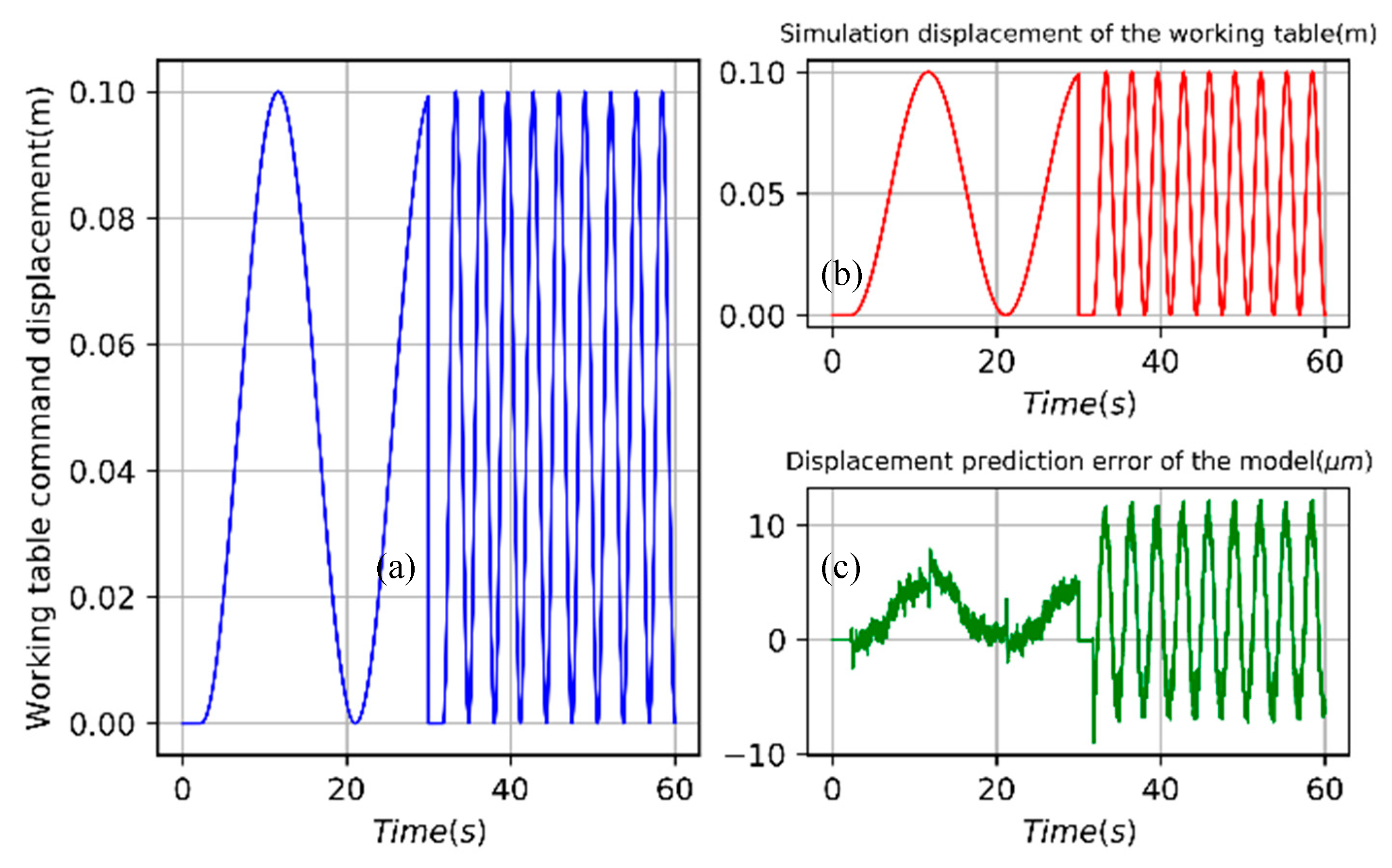
  • The hybrid model was validated using experimental data at different speeds, and the results show that, whether for the tracking error of a single-axis feeding system or the contour error of a double-axis feeding system, the prediction effect of the hybrid model is better than that of a pure analytical model, and the prediction accuracy of the hybrid model reaches a higher level.
The hybrid modeling method combined the advantages of the analytical modeling and the data-driven modeling methods. Complex system models often have numerous parameters, and some parameters are difficult to determine accurately. In addition, pure analytical models generally have assumptions, so pure analytical models inevitably have uncertainties and unmodeled dynamics. Coupling a data-driven model to the multi-domain integrated analytical model of feed systems, the uncertainty of the model can be reduced to a certain extent, and the accuracy of the model can be improved. The research results of this paper could be applied to error compensation control of CNC machine tools to improve their control accuracy.

Author Contributions

Conceptualization, Z.M. and L.C.; methodology, J.D.; validation, T.P. and Z.M.; data curation, J.D.; writing—original draft preparation, Z.M.; writing—review and editing, J.D.; visualization, Z.M. and Z.M.; supervision, L.C.

Funding

This research was funded by [National Key R&D Program of China] grant number [2018YFB1700905].

Conflicts of Interest

The authors declare no conflict of interest.

References

  1. Altintas, Y. Machine tool feed drives. CIRP Ann. 2011, 60, 779–796. [Google Scholar] [CrossRef]
  2. Zhang, H.; Zhang, J.; Liu, H.; Liang, T.; Zhao, W. Dynamic modeling and analysis of the high-speed ball screw feed system. Proc. Inst. Mech. Eng. Part B J. Eng. Manuf. 2015, 229, 870–877. [Google Scholar] [CrossRef]
  3. Erkorkmaz, K.; Kamalzadeh, A. High bandwidth control of ball screw drives. CIRP Ann. 2006, 55, 393–398. [Google Scholar] [CrossRef]
  4. Tsai, P.C.; Cheng, C.C.; Hwang, Y.C. Ball screw preload loss detection using ball pass frequency. Mech. Syst. Signal Process. 2014, 48, 77–91. [Google Scholar] [CrossRef]
  5. Zhang, C.Y.; Chen, Y.L. Tracking control of ball screw drives using ADRC and equivalent-error-model-based feedforward control. IEEE Trans. Ind. Electron. 2016, 63, 7682–7692. [Google Scholar] [CrossRef]
  6. Sepasi, D.; Nagamune, R. Tracking control of flexible ball screw drives with runout effect and mass variation. IEEE Trans. Ind. Electron. 2012, 59, 1248–1256. [Google Scholar] [CrossRef]
  7. Armstrong-Hélouvry, B.; Dupont, P.; DeWit, C.C. A survey of models, analysis tools and compensation methods for the control of machines with friction. Automatica 1994, 30, 1083–1138. [Google Scholar] [CrossRef]
  8. Jeong, H.Y.; Min, B.K.; Cho, D.W.; Lee, S.J. Motor current prediction of a machine tool feed drive using a component-based simulation model. Int. J. Precis. Eng. Manuf. 2010, 11, 597–606. [Google Scholar] [CrossRef]
  9. Karnopp, D. Computer simulation of stick-slip friction in mechanical dynamic systems. ASME J. Dyn. Syst. Meas. Control 1985, 107, 100–103. [Google Scholar] [CrossRef]
  10. Duan, M. Dynamic Modeling and Experiment Research on Twin Ball Screw Feed System Considering the Joint Stiffness. Symmetry 2018, 10, 686. [Google Scholar] [CrossRef]
  11. Johanastrom, K.; Canudas-de-Wit, C. Revisiting the LuGre friction model. IEEE Control Syst. Mag. 2008, 28, 101–114. [Google Scholar] [CrossRef] [Green Version]
  12. Grundelius, M.; Angeli, D. Adaptive control of systems with back-lash acting on the input. In Proceedings of the 35th IEEE Conference on Decision and Control, Kobe, Japan, 13 December 1996; pp. 4689–4694. [Google Scholar]
  13. Tao, G.; Ma, X.; Ling, Y. Optimal and nonlinear decoupling control of systems with sandwiched backlash. Automatica 2001, 37, 165–176. [Google Scholar] [CrossRef]
  14. Mata-Jimenez, M.T.; Brogliato, B.; Goswami, A. On the control of mechanical systems with dynamic backlash. In Proceedings of the 36th IEEE Conference on Decision and Control, San Diego, CA, USA, 12 December 1997; pp. 1990–1995. [Google Scholar]
  15. Kamalzadeh, A.; Erkorkmaz, K. Compensation of axial vibrations in ball screw. CIRP Ann. Manuf. Technol. 2007, 56, 373–378. [Google Scholar] [CrossRef]
  16. Tsai, M.S.; Huang, Y.C.; Lin, M.T.; Wu, S.K. Integration of input shaping technique with interpolation for vibration suppression of servo-feed drive system. J. Chin. Inst. Eng. 2017, 40, 284–295. [Google Scholar] [CrossRef]
  17. Huang, H.W.; Tsai, M.S.; Huang, Y.C. Modeling and elastic deformation compensation of flexural feed drive system. Int. J. Mach. Tools Manuf. 2018, 132, 96–112. [Google Scholar] [CrossRef]
  18. Li, F.; Jiang, Y.; Li, T. An improved dynamic model of preloaded ball screw drives considering torque transmission and its application to frequency analysis. Adv. Mech. Eng. 2017, 9, 1687814017710580. [Google Scholar] [CrossRef]
  19. Xu, Z.Z.; Choi, C.; Liang, L. Study on a novel thermal error compensation system for high-precision ball screw feed drive (2 nd report: Experimental verification). Int. J. Precis. Eng. Manuf. 2015, 16, 2139–2145. [Google Scholar] [CrossRef]
  20. Pislaru, C.; Derek, G.F.; Holroyd, G. Hybrid modelling and simulation of a computer numerical control machine tool feed drive. Proc. Inst. Mech. Eng. Part I J. Syst. Control Eng. 2004, 218, 111–120. [Google Scholar] [CrossRef]
  21. Whalley, R.; Ebrahimi, M.; Abdul-Ameer, A.A. Hybrid modelling of machine tool axis drives. Int. J. Mach. Tools Manuf. 2005, 45, 1560–1576. [Google Scholar] [CrossRef]
  22. Whalley, R.; Abdul-Ameer, A.A.; Ebrahimi, M. Machine tool modelling and profile following performance. Appl. Math. Model. 2008, 32, 2290–2311. [Google Scholar] [CrossRef]
  23. Zaeh, M.F.; Oertli, T.; Milberg, J. Finite element modelling of ball screw feed drive systems. CIRP Ann. Manuf. Technol. 2004, 53, 289–292. [Google Scholar] [CrossRef]
  24. Yang, X. Electromechanical integrated modeling and analysis for the direct-driven feed system in machine tools. Int. J. Adv. Manuf. Technol. 2018, 98, 1591–1604. [Google Scholar] [CrossRef]
  25. Zhang, X. Integrated modeling and analysis of ball screw feed system and milling process with consideration of multi-excitation effect. Mech. Syst. Signal Process. 2018, 98, 484–505. [Google Scholar] [CrossRef]
  26. Maj, R.; Bianchi, G. Mechatronic analysis of machine tools. In Proceedings of the 9th SAMTECH Users Conference, Paris, France, 2–3 February 2005; pp. 2–3. [Google Scholar]
  27. Ansoategui, I.; Campa, F.J. Mechatronics of a ball screw drive using an N degrees of freedom dynamic model. Int. J. Adv. Manuf. Technol. 2017, 93, 1307–1318. [Google Scholar] [CrossRef] [Green Version]
  28. Kim, M.S.; Chung, S.C. A systematic approach to design high-performance feed drive systems. Int. J. Mach. Tools Manuf. 2005, 45, 1421–1435. [Google Scholar] [CrossRef]
  29. Herfs, W. Design of Feed Drives with Object-Oriented Behavior Models. IFAC-PapersOnLine 2015, 48, 268–273. [Google Scholar] [CrossRef]
  30. Luo, W. Digital twin for CNC machine tool: modeling and using strategy. J. Ambient Intell. Humaniz. Comput. 2019, 10, 1129–1140. [Google Scholar] [CrossRef]
  31. Özdemir, D. Modelica Library for Feed Drive Systems. In Proceedings of the 11th International Modelica Conference, Versailles, France, 21–23 September 2015; Linköping University Electronic Press: Linköping, Sweden, 2015; pp. 117–125. [Google Scholar]
  32. Jordan, M.I.; Mitchell, T.M. Machine learning: Trends, perspectives, and prospects. Science 2015, 349, 255–260. [Google Scholar] [CrossRef]
  33. Wuest, T.; Weimer, D.; Irgens, C. Machine learning in manufacturing: advantages, challenges, and applications. Prod. Manuf. Res. 2016, 4, 23–45. [Google Scholar] [CrossRef] [Green Version]
  34. Li, Z.; Wang, Y.; Wang, K. A data-driven method based on deep belief networks for backlash error prediction in machining centers. J. Intell. Manuf. 2017, 1–13. [Google Scholar] [CrossRef]
  35. Chiu, H.W.; Lee, C.H. Prediction of machining accuracy and surface quality for CNC machine tools using data driven approach. Adv. Eng. Softw. 2017, 114, 246–257. [Google Scholar] [CrossRef]
  36. Park, J.; Law, K.H.; Bhinge, R. A generalized data-driven energy prediction model with uncertainty for a milling machine tool using Gaussian Process. In Proceedings of the ASME 2015 International Manufacturing Science and Engineering Conference, Charlotte, NC, USA, 8–12 June 2015. [Google Scholar]
  37. Ziegert, J.C.; Kalle, P. Error compensation in machine tools: a neural network approach. J. Intell. Manuf. 1994, 5, 143–151. [Google Scholar] [CrossRef]
  38. Ak, R.; Helu, M.M.; Rachuri, S. Ensemble neural network model for predicting the energy consumption of a milling machine. In Proceedings of the ASME 2015 International Design Engineering Technical Conferences and Computers and Information in Engineering Conference, Boston, MA, USA, 2–5 August 2015. [Google Scholar]
  39. Yan, J.; Lee, J. Degradation assessment and fault modes classification using logistic regression. J. Manuf. Sci. Eng. 2005, 127, 912–914. [Google Scholar] [CrossRef]
  40. Carbonneau, R.; Laframboise, K.; Vahidov, R. Application of machine learning techniques for supply chain demand forecasting. Eur. J. Oper. Res. 2008, 184, 1140–1154. [Google Scholar] [CrossRef]
  41. Hou, Z.; Gao, H.; Lewis, F.L. Data-Driven Control and Learning Systems. IEEE Trans. Ind. Electron. 2017, 64, 4070–4075. [Google Scholar] [CrossRef]
  42. Park, J.; Ferguson, M.; Law, K.H. Data Driven Analytics (Machine Learning) for System Characterization, Diagnostics and Control Optimization//Workshop of the European Group for Intelligent Computing in Engineering; Springer: Cham, Switzerland, 2018; pp. 16–36. [Google Scholar]
  43. Reinhart, R.; Shareef, Z.; Steil, J. Hybrid analytical and data-driven modeling for feed-forward robot control. Sensors 2017, 17, 311. [Google Scholar] [CrossRef]
  44. Reinhart, R.F.; Steil, J.J. Hybrid mechanical and data-driven modeling improves inverse kinematic control of a soft robot. Procedia Technol. 2016, 26, 12–19. [Google Scholar] [CrossRef]
  45. Chikh, K.; Saad, A.; Khafallah, M. PMSM vector control performance improvement by using pulse with modulation and anti-windup PI controller. In Proceedings of the 2011 International Conference on Multimedia Computing and Systems, Ouarzazate, Morocco, 7–9 April 2011; pp. 1–7. [Google Scholar]
  46. Sebastian, T.; Slemon, G.R. Transient modeling and performance of variable-speed permanent-magnet motors. IEEE Trans. Ind. Appl. 1989, 25, 101–106. [Google Scholar] [CrossRef]
  47. Tu, X.; Zhou, Y.F.; Zhao, P. Modeling the static friction in a robot joint by genetically optimized BP neural network. J. Intell. Robot. Syst. 2019, 94, 29–41. [Google Scholar] [CrossRef]
Figure 1. Connection mechanism of the component models.
Symmetry 11 01156 g001
Figure 2. Module division of the ball screw feed system driven by a permanent magnet synchronous motor (PMSM).
Symmetry 11 01156 g002
Figure 3. Structure of the multi-domain analytical model of the ball screw feed system.
Symmetry 11 01156 g003
Figure 4. Illustration for the schematic diagram of the mechanical subsystem.
Symmetry 11 01156 g004
Figure 5. The nonlinearity of the backlash model.
Symmetry 11 01156 g005
Figure 6. Illustration for the modeling of space vector pulse width modulation (SVPWM) and inverter.
Symmetry 11 01156 g006
Figure 7. Equivalent circuit of PMSM. (a) Equivalent circuit of d axis; (b) Equivalent circuit of q axis.
Symmetry 11 01156 g007
Figure 8. Training data for the back propagation neural network (BPNN). (a) Input data of position command; (b) Input data of analytical simulated position; (c) Output data of deviation.
Symmetry 11 01156 g008
Figure 9. Training results of the BPNN.
Symmetry 11 01156 g009
Figure 10. Schematic diagram of the hybrid modeling method.
Symmetry 11 01156 g010
Figure 11. The hybrid model of the ball screw feed system.
Symmetry 11 01156 g011
Figure 12. Experiment platform of the ball screw feed system.
Symmetry 11 01156 g012
Figure 13. The position command signal of the workbench.
Symmetry 11 01156 g013
Figure 14. Comparison of the pure analytical model simulation results and the hybrid model simulation results at different feed speed.
Symmetry 11 01156 g014
Figure 15. Comparisons between simulation results and experimental results of circular trajectory tracking at different velocity.
Symmetry 11 01156 g015
Figure 16. Comparison of contour error predicted by pure analytical model and hybrid model at different velocities.
Symmetry 11 01156 g016
Table 1. Connector defined in each subject area.
Mechanical ConnectorsElectrical ConnectorsControl Connectors
IconIcon Icon
Flow variableTorque τFlow variableCurrent iInput variable u
Potential variableAngle φPotential variableVoltage vOutput variable y
Table 2. The parameters of the ball screw feed system.
Name of ParametersValue
Nominal torque of the motor18 N m
Nominal speed of the motor2000 rpm
Nominal current of the motor12.5 A
Nominal power of the power3.6 Kw
Inertia of the motor rotor5.3 ×   10 3   Kg m 2
Pole-pair number of the motor4
Equivalent resistance of phase winding0.184   Ω
d axis inductance of the motor L d 2.3 ×   10 3 H
q axis inductance of the motor L q 2.3 ×   10 3   H
Control cycle of position loop0.001 s
Position loop gain120 Hz
Control cycle of velocity loop0.125 ms
Velocity loop gain800 Hz
Integral time constant of velocity loop40 ms
Control cycle of current loop31.25 us
Current loop gain5000 Hz
Integral time constant of current loop9.8 ms
DC-side voltage of inverter560 V
Pitch of the ball screw16 mm
backlash17 um
Table 3. Simulation accuracy of the hybrid model at different feeding rate.
Feed Rate (mm/min)F1000F2000F3000F4000F5000F6000
Hybrid model(MAE)/ μ m 5.225.165.985.274.556.79
(RMSE)/ μ m 1.872.331.721.411.642.63
(RE)2.7%2.0%1.1%0.7%0.5%0.6%
Analytical model(MAE)/ μ m 7.997.527.708.5110.212.38
(RMSE)/ μ m 2.912.833.153.844.896.21
(RE)4.2%4.0%1.4%1.1%1.1%1.2%
Table 4. Comparison of maximum contour error predicted by analytical model and hybrid model at different velocity.
ω   ( rad / min ) 6080100120
Max Error (Analytical model predicted)/ μ m 7.198.6210.2612.54
Max Error (Hybrid model predicted)/ μ m 6.575.344.106.95

