Multi-Aspect Embedding for Attribute-Aware Trajectories


1
University of Chinese Academy of Sciences, Beijing 100049, China
2
Key Lab of Intelligent Information Processing of Chinese Academy of Sciences (CAS), Institute of Computing Technology, Chinese Academy of Sciences, Beijing 100190, China
*
Authors to whom correspondence should be addressed.
Symmetry 2019, 11(9), 1149; https://doi.org/10.3390/sym11091149
Submission received: 15 August 2019
/
Revised: 31 August 2019
/
Accepted: 3 September 2019
/
Published: 10 September 2019
Abstract
:Motivated by the proliferation of trajectory data produced by advanced GPS-enabled devices, trajectory is gaining in complexity and beginning to embroil additional attributes beyond simply the coordinates. As a consequence, this creates the potential to define the similarity between two attribute-aware trajectories. However, most existing trajectory similarity approaches focus only on location based proximities and fail to capture the semantic similarities encompassed by these additional asymmetric attributes (aspects) of trajectories. In this paper, we propose multi-aspect embedding for attribute-aware trajectories (MAEAT), a representation learning approach for trajectories that simultaneously models the similarities according to their multiple aspects. MAEAT is built upon a sentence embedding algorithm and directly learns whole trajectory embedding via predicting the context aspect tokens when given a trajectory. Two kinds of token generation methods are proposed to extract multiple aspects from the raw trajectories, and a regularization is devised to control the importance among aspects. Extensive experiments on the benchmark and real-world datasets show the effectiveness and efficiency of the proposed MAEAT compared to the state-of-the-art and baseline methods. The results of MAEAT can well support representative downstream trajectory mining and management tasks, and the algorithm outperforms other compared methods in execution time by at least two orders of magnitude.
1. Introduction
With the growth of mobile computing and advances in location-acquisition techniques, a large number of trajectories are continuously being acquired. In general, a trajectory, which consists of a finite chronological sequence of coordinates, records the traveling history of a moving object such as a person, vehicle, animal, etc., Mining trajectories were studied for decades and underpinned various real-world applications, e.g., animal migration analysis [1], air traffic management [2], hurricane prediction [1], traffic planning [3], urban computing [4,5,6], etc., [7,8]. Measuring similarities among trajectories functions as one of the backbones in many trajectory management and mining tasks [1,2,3,7,8].
Traditional methods measure the similarity between two trajectories by forming pairwise point-matching strategies [9,10,11,12,13].
Despite the remarkable successes of existing pairwise point-matching approaches, they suffer from several imperfections especially when trajectories have low/non-uniform sampling rates and are affected by noise. For instance, we demonstrate an example in Figure 1 in which four trajectories with different sampling rates are exhibited. In this figure, though and are produced from the same underlining route, they might be judged as dissimilar by existing point-matching methods since contains a noise point, namely . Furthermore, although and demonstrate two trajectories representing the same underlying route, the conventional point-matching methods may have difficulties to identifying their similarities due to their distinct sampling rates and the low-sampling rate of .
Recently, trajectory embedding methodologies [14,15,16] are proposed to address the defects of point-matching approaches. These methods attempt to learn a mapping function that transfers trajectories into low-dimensional and dense vector representations in which the “similar” trajectories are close to each other while the “dissimilar” ones are far away. The concrete similarities are mainly defined on the geographical correlativeness of trajectories [14,15], i.e., the distance of coordinates. However, with the spread of advanced GPS-enabled devices, e.g., smartphones/smartwatches, and emerging apps deployed on these platforms, trajectories become more complex and begin to embroil additional attributes beyond only the coordinates. For example, timestamps when passing through the coordinates, geo-tags of the coordinates provided by map APIs, temperature during the travel at the coordinates measured by thermosensors, and user generated text/images at specific coordinates could all be recorded. These asymmetric attributes may provide useful side information for real-world applications, indicating semantic correlations among trajectories. Take the trajectories , and in Figure 1 as an example. Though and share the underlining routes (only spatial factor), and could be more similar if spatial and temporal factors are simultaneously considered as and share the same destination, and both of them are generated at the rush hours in the morning. In the above example, temporal together with the spatial correlativeness of trajectories may unearth fine-grained human mobility patterns in cities and could further motivate strategies for urban management.
Motivated by such observations, in this paper, we propose multi-aspect embedding for attribute-aware trajectories (MAEAT) in which multiple aspects of trajectories are jointly considered. Here aspects contain not only the traditional spatial coordinates, but also attributes of trajectory data. In this paper, we will use the terms “aspect” and “attribute” interchangeably. For simplicity, we adopt only two aspects, namely spatial and temporal aspects, in this paper. However, our method could be easily extended to other aspects. MAEAT offers a flexible design to encode multiple attributes of trajectories into a unified representation such that similar trajectories are placed closely to each other in the latent space according to their extracted aspects.
Specifically, MAEAT consists of two stages. First, the algorithm extracts multiple aspects from the raw trajectories. These aspects are discrete tokens that characterize the trajectory data. A hidden Markov model-based mapping method and a kernel-based clustering approach are adopted to transfer the continuous aspects, i.e., coordinates and timestamps, into discrete tokens, respectively. Second, a learning method is proposed to integrate the multi-aspect tokens and generate embedding vectors for the trajectory data. The learning process is inspired by sentence embedding [17] that learns via predicting the context words for a sentence, i.e., sentences are similar when they contain similar key words. We naturally project every aspect token as a word and a whole trajectory as a sentence. However, unlike sentence embedding, MAEAT is designed to simultaneously incorporate more than one aspect token, and we devise a regularization method to control the importance among aspects and to alleviate the aspect imbalance problem during the training.
Extensive experiments on both synthetic and real-world datasets demonstrate the effectiveness of the proposed MAEAT. Specifically, the output embedding produced by MAEAT can support representative downstream data mining and pattern recognition tasks such as clustering and k-nearest neighbour query (kNN). We also found that it runs faster than the compared point-matching methods by two orders of magnitude (refer to Section 5.2.3).
2. Related Work
We categorize related papers in the literature as follows:
Trajectory similarity computations.
Extensive studies on trajectory similarity have been carried out over the past decade. Euclidean distance [13] of sampled data points was first used to measure the similarity between two trajectories. However, it fails to handle local time shifting, which is crucial in measuring the similarity of trajectories. In addition, it needs the two trajectories to have the same length which is usually impractical with a real database. Dynamic time warping (DTW) [10] was the first method to measure the similarity by finding the best alignment between points in two trajectories with different lengths. Edit distance on real sequence (EDR) [12], edit distance with real penalty (ERP) [9], longest common subsequence (LCSS) [11] and MA model [18] achieved other improved point-matching approaches which attempted to buoy the effectiveness and the efficiency of the previous methods. However, these methods calculate distances based on sampled points, thus they might not be robust to noises or non-uniform sampled points. Recall that the sampled points of trajectories could be drifted due to power constraints, disrupted network connections, etc. Moreover, the performances of EDR, ERR, LCSS, and MA heavily rely on parameters; slight changes of the parameters could have a significant influence on the calculated distances. Edit distance with projection (EDwP) [19] is a recent parameter-free approach to tackle the problem of sampling rate inconsistency in which “insert” and “replace” operations of points are alternately performed to seek the optimally aligned segments. In addition, the trajectory calibration approach [20] aligns trajectories to a set of anchor points as a stable reference system to deal with the different sampling strategy issues of the heterogeneous trajectories in the database. Recently, NeuTraj [21] was proposed to approximate the similarity computations of trajectories in linear time and gain significant performance improvement compared to other existing approaches, such as DTW, and EDR. DISON [22] was introduced to compute the similarity between two on-road trajectories by considering the LCSS score between the sequence of road segments derived from the two trajectories.
Trajectory representation learning.
Representation learning for trajectory data [14,15,16,23,24,25,26,27] has attracted the attention of researchers and has become an emerging topic. Li et al., proposed t2vec [14], which learns embedding vectors for trajectories based on the recurrent neural network-based denoising autoencoder through a reconstruction process of raw and disrupted trajectories. Thus, the training process can be time-consuming when performing on a large-scale database since it needs to generate more disrupted training samples. Yang et al., [15] embedded human activity trajectories according to the semantic similarities of activities to find users with similar behaviors. MPE [23] considers the joint action of different attributes and encodes them into an embedding vector. Location2vec [24] learns embedding vectors for urban locations by considering the interaction between urban locations and moving objects. Ying et al., [25] employed Markov chains to capture the strong connections (short geographical distances) to model sequential influence between locations. MC-TEM [16] studies check-in trajectories from which it learns embedding vectors of general contexts for locations. Wang et al., [26] exploited the geographical influence between two locations through three factors, i.e., geo-influence, geo-susceptibility, physical distances of locations, and projected the users and locations into a unified embedded space.
Most of the above methods [15,16,23,24,26] rely on the word embedding (word2vec model) [28] in which they aim to learn the embedding vectors for specific entities, e.g., locations and users, and for specific tasks, e.g., successive location recommendations [15,23], and personalized location recommendations [16,26], etc., [24]. Aggregation mechanisms [29] are usually adopted to obtain the whole trajectory’s embedding vector via combining the embedding vectors of those location entities. However, information loss might be encountered when performing the aggregation. The main difference in our work is that we consider the joint probabilities of multiple aspects as the contexts of the trajectory, and directly learn the embedding vectors for trajectories, rather the component entities in the trajectories. Therefore, our method can remedy the information loss problem and is suitable for similarity computations based on multiple aspects.
3. Preliminaries and Problem Statement
We first give the preliminaries required for our work, and then we proceed to give the problem statement of this paper.
Definition 1.
(Trajectory) A trajectory which shows the traveling history of a moving object is a chronological sequence of states, denoted by T = , where state is a recorded spatial coordinate , and is the length of trajectory.
Definition 2.
(K-aspect Trajectory) Given state in a trajectory T, there exists a set of attributes = , where is the j-th attribute of . We can also include = itself as an attribute reflecting the spatial factor in such that = = , where = K. Given a trajectory T, we define the K-aspect trajectory corresponding to T as = .
For example, considering trajectory = in Figure 1, when spatial and temporal factors are considered, the two-aspect trajectory of is denoted as = 〈[, (08:30 am) ],[, (08:35 am)],[, (08:40 am)]〉, where indicates a temporal instance.
Definition 3.
(K-aspect Sequence) Given a K-aspect trajectory = , a K-aspect sequence of is denoted by τ = 〈,,⋯,〉, where = is the set of K discrete tokens corresponding to in which is the token reflecting the aspect .
Here we give the problem statement of our paper. Given a set of trajectories = containing multiple attributes, we first extract K-aspect sequences (Definition 3) from the trajectories according their states. This K-aspect sequence will reflect the K aspects of trajectory which characterize the trajectory data. Our goal is to learn the representations (a.k.a. low-dimensional embedding vectors) of trajectories to reflect the proximity based on their multiple aspects among trajectories which are simultaneously in the original space.
4. The MAEAT Approach
In this section, we detail the proposed MAEAT. We propose the multi-aspect trajectory embedding method with regularization that controls the importance among K aspects and alleviates the aspect imbalance problem in the training step. Next, we introduce two approaches that extract the aspect components from the raw trajectory data. One is built upon the hidden Markov model which extracts the road network aspect, and the other is a kernel-based clustering method that aims to generate discrete temporal aspects. Figure 2 demonstrates the framework of our MAEAT and Table 1 presents the notations used in this paper.
4.1. Multi-Aspect Embedding with Aspect Regularization
We first describe the embedding method, and assume the K-aspect sequences have been already obtained. Given a set of trajectories = , we first assume that all the trajectories in have been converted to K-aspect sequences (Definition 3). We denote the set of K-aspect sequences by = . The details of the conversion process will be introduced in Section 4.2. The embedding method provides a flexible way to learn the low-dimensional representation vectors based on the multiple aspects to characterize the trajectory data. Specifically, each multi-aspect token () is treated as a context of the trajectory T. Given a K-aspect sequence = 〈,,⋯,〉 which is converted from T, we aim to maximize the log probability of the multi-aspect tokens = in as follows.
can be computed by the joint probability of the K aspects as follows.
We employ a sigmoid function to compute the term = such that = , where is the dot product of two vectors, and , which denote d-dimensional embedding vectors () of token and trajectory T in k-th aspect, respectively. The sigmoid function is defined as , in which it is differentiable and able to generate a non-linear smooth S-shaped curve such that the output value exists between 0 and 1. We choose the sigmoid function because we want to non-linearly model the probability of predicting token given the token sequence .
As the model considers multiple aspects, we employ -regularization to control the importance of each aspect. The -regularization plays a crucial role in mitigating the aspect imbalance problem in the training step, which is defined as follows.
where K is the number of aspects, = is the vocabulary set of the a-th aspect token embedding vectors, is the b-th embedding vector of a-th aspect, and is the tuning parameter that weights the importance of the aspect a. Finally, we aim to minimize the negative log probability of the entire trajectory data as the following objective function.
In our model, we employ stochastic gradient descent (SGD) to optimize the objective function. The parameters to learn in the model are the embedding vectors for every aspect, and trajectories, i.e., . To this end, we aim at minimizing the objective function in Equation (4) by the descending gradient direction, , where is the learning parameters in the model and is the learning rate. In what follows, we give the updated rules based on the partial derivatives of the loss function with respect to the learning parameter .
For a K-aspect sequence = 〈,,⋯,〉 which is converted from T, we calculate the gradients for updating the embedding vectors for trajectory T in the k-th aspect as follows.
For each = , we update the vectors with the following formula:
where . The algorithm goes through every trajectory T in and computes the gradients for trajectory T in K aspects and the K aspect tokens , , ⋯, , and updates their embedding vectors according to Equations (5) and (6), respectively. The algorithm runs until reaching the predetermined iterations () and returns the set of trajectory embeddings in every aspect as the output. The algorithm takes to process every trajectory. For each trajectory, since we need to update K vectors of each aspect and K vectors of the trajectory embedding vectors in each aspect, it requires to update the parameters, where is the average length of trajectories in the dataset. In total, we need to train the model for iterations.
Once all the embedding vectors of trajectories in all aspects have been learned, we will follow the mechanism in [29] to obtain the multi-aspect embedding vectors for all the trajectories in the database.
4.2. Aspect Sequence Acquisition
So far, the remaining problem is how to extract the K-aspect sequence from a given trajectory. In this paper, we adopt two methods to extract spatial and temporal aspects, respectively. Next, we detail these two approaches.
4.2.1. Spatial Aspect Extraction
First, we introduce a hidden Markov model (HMM) map-matching method [30], which can accurately map GPS coordinates to their real road segments. Essentially, the algorithm employs the tradeoff between the road segments suggested by the GPS and the transition probability of the path (from one road segment to the next possible road segments). Figure 3 shows a running example of a road network with GPS points and its corresponding HMM model for the map matching algorithm. In HMM, it regards GPS and road segments as the observations and hidden states, respectively.
First, the algorithm finds k nearest road segments as the candidates for each GPS point, e.g., has two candidates, i.e., road segments and , respectively. We regard these road segment candidates from the previous step as the hidden states corresponding to each GPS point as shown in the diagram in Figure 3 (right). Second, the algorithm computes the emission probabilities between GPS and road segments, i.e., = , where is the projected point of the point on the road segment , and is an estimated standard deviation. We can see this probability will become higher when the point is close to the road segments. Third, the algorithm computes the transition probabilities between road segments, i.e., a high probability means the selected road segment is reasonable to travel. It can be calculated by = , where d is the difference between the great circle distance and route distance on the road network graph, and is another estimated parameter. Finally, the algorithm employs the Viterbi algorithm to find the most likely sequence of road segments on the HMM. For example, in Figure 3, the selected road path for the trajectory contains the points is .
We can see this method maps the GPS points to the most reasonable road segments by carefully accounting for the road constraints and being able to handle noises and different sampling rates. Thus, we can accurately partition the trajectories into a discrete sequence of road segments and derive the spatial aspect sequences of the trajectories of moving objects on roads.
4.2.2. Temporal Aspect Extraction
Next, we introduce how to acquire temporal aspect sequences. We adopt a density-based clustering method that is built upon the mean shift clustering algorithm [31]. Specifically, we first identify the temporal hotspots from the database using kernel density estimation (KDE) [32], which is a non-parametric method estimating the density function based on the finite observed data without requiring any prior knowledge of the data distribution. In more detail, given n timestamps , the kernel density at any time t is given by
where is a kernel function and h is the kernel bandwidth. Though there are many kernel functions that can be used, we choose the Gaussian kernel due to its simplicity and the empirical assumption that the temporal factor is under the Gaussian distribution. The Gaussian kernel is given by , and the temporal hotspots can be identified by the local maximum of the density estimated by the kernel.
We extract temporal aspects by employing the mean shift algorithm [31] to find the corresponding mode by iteratively shifting a radius-h window towards a local density maxima. Through this manner, we can group every timestamp into appropriate clusters. Figure 4 shows an example of temporal clustering. We randomly sample 300 timestamps of trajectories and perform the clustering algorithm on the data. From the figure, we have discovered three temporal clusters shown by the black cross (×) symbols while the time instances are illustrated by the red plus (+) symbols. We can notice that each cluster will correspond to the local peak of the density function, and we could assign the corresponding cluster ID to every timestamp as its temporal token and concatenate these tokens to form a temporal aspect sequence of a trajectory.
5. Experiments
In this section, we evaluate our proposed framework on five benchmark datasets and one real-world trajectory dataset of taxis. We examine both the effectiveness and efficiency of the proposed methods through quantitative and qualitative analysis.
5.1. Experimental Settings
The experiments were conducted on a computer equipped with four Intel (R) Core (TM) i7-7700HQ CPU @2.80GHz 8 GB RAM running a Windows 10 operating system. For the road network construction and map matching algorithms, we modify the codes which are publicly available from the website of UIC (https://www.cs.uic.edu/bin/view/Bits/Software).
5.1.1. Datasets
We obtain the benchmark datasets from [33] and a real taxi dataset in the city of Porto (http://www.geolink.pt/ecmlpkdd2015-challenge/). The benchmark datasets have ground truth while the Porto dataset does not. The data statistical information is illustrated in Table 2. i5sim and i5sim3 contain the trajectory data on highways which result in eight and 16 clusters, respectively. cross and cross2 are trajectories across an intersection and have 19 and 13 clusters, respectively. The major difference between these two datasets is that the trajectories traveling through the same road segments are grouped in the same clusters on cross2. For cross3, we randomly generate timestamps for each point of trajectories in cross2, and derive 39 clusters not only according to the similarity in terms of locations, but also the correlativeness of temporal factors. Porto is a real dataset containing about 1.7 million trajectories from 442 taxis in the city of Porto, in Portugal. The trajectories of the Porto dataset contain sampled points with an even time interval (15 s). Trajectories that contain less than 30 sampled points are excluded from the dataset, and we randomly picked 5000 trajectories as our testbed.
5.1.2. Compared Methods
We evaluate the effectiveness and efficiency of the compared methods, and they can be divided into five categories: the point-matching methods, the road-network-aware method, the encoder-decoder based methods, word2vec-based method, and the newly proposed methods.
- Point-matching methods: Dynamic time warping (DTW), edit distance with real penalty (ERP), longest common subsequences (LCSS) are compared since they are widely adopted methods for trajectory similarity computation.
- Road-network-aware method: DISON [22] is a recent road-network-aware method which computes the similarity based on LCSS score between sequences of road segments.
- Encoder-decoder methods: Recurrent neural network (RNN), gated recurrent unit (GRU) and long-short term memory (LSTM) are compared as three basic encoder-decoder methods. Moreover, we compare T2vec [14] which is a state-of-the-art trajectory embedding method based on the encoder-decoder architecture (https://github.com/boathit/t2vec).
- MAEAT, the methods proposed in this paper: A variant of the proposed MAEAT is meanwhile compared in which only the spatial aspect is considered. We involve such a variant not only for illustrating the effectiveness of multiple aspect embedding but also for the ablation test. We denote this degraded version as MAEAT(S).
5.1.3. Parameters
For the embedding vector size and the hidden layer size, we fix them at 200 for all the embedding-based models. EDR and LCSS require in their algorithms, we also perform the grid search to specify that produces the best results. For T2Vec and MC-TEM, we retain the settings as suggested in the papers with a slight change to fit our experiments.
5.2. Experimental Analysis
In this section, we provide both quantitative and qualitative analysis.
5.2.1. Quantitative Analysis
We first quantitatively examine the effectiveness of the compared methods by running a clustering algorithm on the resultant trajectory embeddings, where the k-means is employed on the embedding-based methods. For the point-matching methods, there are no corresponding trajectory embeddings, thus we directly perform the spectral clustering on the similarity matrix which is computed by these point-matching methods. All the benchmark datasets are evaluated since they have ground truth. We only report the result of our MAEAT on cross3 since the other datasets do not contain timestamps.
To evaluate the clustering accuracy, we employ two well-known validity measures, i.e., purity and adjusted rand index (ARI). Purity measures the maximized correct mapping rate of the clustering results and the ground truth.
where is the set of ground truth clusters, is the set of result clusters, N and k are the size of dataset and the number of ground truth clusters, respectively. While purity measures the maximized correct mapping rate, ARI cares more about the objects in their different clusters. The calculation of ARI is given as follows.
where , and .
Table 3 shows the clustering performances of the compared methods, and the best performances are highlighted in bold face. First, we observe that MAEAT(S) and MAEAT can outperform almost all the compared methods on both measures over most of the benchmarks. Without considering temporal factors, the degraded MAEAT(S) clearly runs better than the point-matching methods, the road-network-aware method, and the encoder-decoder methods. Though MC-TEM achieves better performance on cross and cross3 than MAEAT(S), our full model MAEAT significantly improves the performance on cross3, as it simultaneously considers multiple aspects in the trajectory embedding process. For baselines, we observe all the compared methods are perfectly accurate on the simplest dataset i5sim. DTW, as the most representative point-matching based method, is more stable than the others. LCSS performs the best on cross, and we conjecture the reason is due to it having the longest common subsequence alignment. For encoder-decoder based methods, we see that they fail to perform very well on this task, even the recent T2Vec. We analyze the reason and find that the trajectories in these benchmarks have varied lengths, and the time intervals between two consecutive points could be different, which might challenge these methods to learn a robust trajectory representation. The word2vec based method, MC-TEM, achieves better performance among the baselines. However, MC-TEM needs to aggregate every token’s embedding together to get the trajectory embedding and the merging strategy may result in information loss. In contrast, our model directly learns the representation of whole trajectories that simultaneously preserve proximities of multiple trajectory attributes. This results in better results.
5.2.2. Qualitative Analysis
We next qualitatively verify the effectiveness of the compared methods by performing a nearest neighbour query. We randomly pick a trajectory and use it as the query to retrieve the trajectories from the testbed whose similarity scores are ranked at top five to visualize as shown in Figure 5. In the figure, the query is shown in the navy thick line, and the other five lines with different colors (each color indicates a similarity ranking score between the retrieved trajectory and the query) are the nearest neighbour trajectories.
Though the dataset has no ground truth, we could visualize the returned nearest neighbour trajectories and check whether they fit to the query on either spatial or temporal factors. From the figure, our proposed methods can return similar results to the query. All the results returned by MAEAT(S) and MAEAT have their beginning points close to that of the query. In addition, the main portions of the results are lying on the query since our methods can take advantage of the map-matching method when extracting spatial aspects. For baselines, we unsurprisingly find that the point-matching based methods are good at such comparisons. Excepting for EDR, which retrieves one trajectory that does not lie on the query, the others can retrieve all five trajectories that have main portions lying on the query with their slight differences in the beginning and ending portions. Recall that these approaches are specifically designed for trajectory similarity computation. Our methods are comparable to them and can underpin more widely in downstream trajectory mining and perform management tasks better. Moreover, we observe both encoder-decoder based and word2vec based methods perform worse than the others in such comparison. Though they could return a small number of similar trajectories, dissimilar ones are meanwhile affected by noises in the results. Furthermore, we can observe that MAEAT(S) and DISON, which consider the road network to compute the similarity, have three similar results, while the remaining two trajectory results of MAEAT(S) are better fits to the query than that of DISON.
5.2.3. Efficiency Evaluation
We now examine the efficiency of the compared methods. We divide this experiment into two parts: (1) training and (2) similarity computation. It is worth noting that all the run times are reported in log scale. For the first part, we compare the run times of the training of LSTM, T2Vec, MC-TEM, MAEAT(S) and MAEAT as the embedding vector size is increased in Figure 6a. We recorded the training time of the compared methods until they produced stable results.
First, we observe that the training phase of T2Vec runs the slowest. For example, T2Vec runs slower than LSTM, MAEAT(S), and MAEAT, when the embedding size is 200, respectively. The reason is that T2Vec generates more disrupted samples to train as the embedding size increases, which results in the worst performance in terms of run time. Moreover, LSTM and MC-TEM run above two orders of magnitude slower than MAEAT(S) and MAEAT in most cases of the embedding sizes. Additionally, we notice that MAEAT runs only slower than MAEAT(S), and the run time linearly grows as the embedding size is increased. This observation suggests a good scalability to the number of aspects and the embedding size.
For the second part, we compared the run times of the similarity computation among the point-matching and embedding-based methods. The experimental results are shown in Figure 6b. In this experiment, we randomly picked a trajectory with a different length, i.e., 60–100, 101–200, 201–300, as the queries and compute the similarity scores with the other 5000 trajectories in the testbed and record their run times. The reported time is the five-time-run average value. Since the performance of DISON is redundant with LCSS, we only report the run time of LCSS in this experiment.
We employ Euclidean and Cosine scores as similarity metrics between the embedding vectors produced by the embedding-based methods. The run times of Euclidean and Cosine computations are represented by E-X and C-X, respectively, in the figure, where X is the embedding vector size. For example, E-200 means we employed the Euclidean similarity score with embedding vectors of size 200. We observe that the run time of point-matching methods increases when the length of the query is longer, while that of embedding-based methods remains stable on both Euclidean and Cosine score computations. For example, DTW runs slower when the query length is increased from 60–100 to 201–300, while the run times of the embedding-based models are stable. Next, we notice that the embedding size does not have much effect on the run times of both Euclidean and Cosine score computation. For example, E-200 and C-200 run only , slower than E-50 and C-50 (the query length = 60–100), respectively. The similar observation can also be found in the other query lengths. Finally, we found that point-matching methods run significantly slower than embedding-based methods. For example, EDR runs , slower than E-200 and C-200 (the query length = 101–200), respectively.
5.2.4. Effects of Regularization
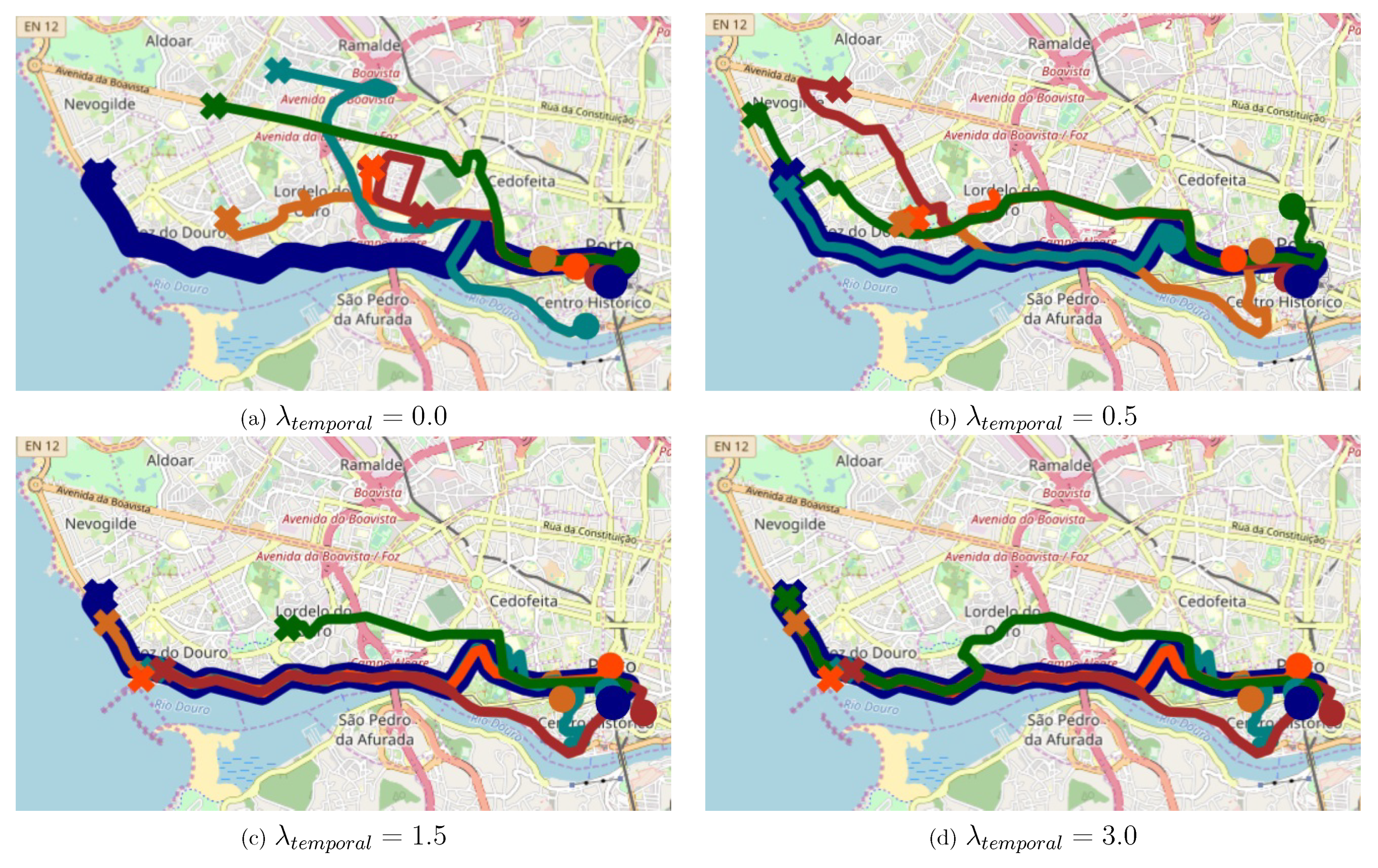
In this section, we aim to show the effects of the regularization. We perform the five-nearest-neighbour query on MAEAT with road and temporal hotspots as its learning aspects. Figure 7 shows the visualization with different settings of , i.e., . There are only six time clusters, while there are more than 9000 different road segments in the training. Thus, according to the learning algorithm presented in Section 4.1, time vectors will have the possibility to be updated more frequently than road segment vectors. This causes the time aspect to dominate the road-segment aspect. This phenomenon is coined as an aspect imbalance problem. The regularization is used to remedy this problem. Specifically, when is increased, the learning algorithm will penalize the importance of the learning of time vectors. From Figure 7a–c, we can see that the algorithm can retrieve the trajectories that are fitter to the query from the spatial perspective when is increased.
When setting , some retrieved trajectories seem not fit the query from the road segment perspective. However, we notice that their start points are in a similar area with the query, and the retrieved trajectories still have strong temporal relevance with the query. Thus the regularization with the model might be helpful for human traffic behavior analysis applications as well as other tasks, especially in urban computing.
6. Conclusions
In this paper, we presented a MAEAT algorithm to study embedding vectors for trajectory data. MAEAT is able to learn the embedding vectors representing trajectories in a latent space according to their joint contextual features (aspects). Two kind of aspects, as a specific example, are explored in MAEAT, and a regularization is equipped on MAEAT to control the importance of each aspect. We carried out the experiments to provide both quantitative and qualitative analysis on both benchmark and real datasets to show the efficiency and effectiveness of our algorithm compared to the state-of-the-art and baseline methods.
Several interesting problems for future research exist. In this paper, we mainly focused on two aspects, i.e., temporal and spatial factors. It is interesting to extend the proposed MAEAT to explore the other attributes of trajectory data such as images, text, and temperature. Next, it would be interesting to employ MAEAT to support other downstream tasks, e.g., popular route query, trajectory search&join, trajectory range query, and real-time route recommendation.
Author Contributions
Conceptualization, T.B. and X.A.; Formal analysis, T.B.; Investigation, T.B.; Methodology, T.B.; Resources, Q.H.; Software, T.B.; Supervision, X.A. and Q.H.; Visualization, T.B. and X.A.; Writing–original draft, T.B.; Writing–review & editing, T.B., X.A. and Q.H.
Funding
The research work supported by the National Key Research and Development Program of China under Grant No. 2017YFB1002104, the National Natural Science Foundation of China under Grant No. U1811461, 61602438, 91846113, 61573335, the Project of Youth Innovation Promotion Association CAS.
Acknowledgments
The authors would like to thank Royal Thai Government Scholarship Program for supporting this research work. The authors would also like to thank the anonymous reviewers for their valuable comments and suggestions. Any findings, opinions, and conclusions in this publication are of those the authors and do not necessarily reflect the views of the funding agencies.
Conflicts of Interest
The authors declare no conflict of interest.
References
- Lee, J.G.; Han, J.; Whang, K.Y. Trajectory Clustering: A Partition-and-group Framework. In Proceedings of the 2007 ACM SIGMOD International Conference on Management of Data, Beijing, China, 11–14 June 2007; ACM: New York, NY, USA, 2007; pp. 593–604. [Google Scholar] [CrossRef]
- Andrienko, G.; Andrienko, N.; Fuchs, G.; Garcia, J.M.C. Clustering Trajectories by Relevant Parts for Air Traffic Analysis. IEEE Trans. Vis. Comput. Graph. 2018, 24, 34–44. [Google Scholar] [CrossRef] [PubMed]
- Lee, J.G.; Han, J.; Li, X.; Gonzalez, H. TraClass: Trajectory Classification Using Hierarchical Region-based and Trajectory-based Clustering. Proc. VLDB Endow. 2008, 1, 1081–1094. [Google Scholar] [CrossRef]
- Xia, T.; Yu, Y.; Xu, F.; Sun, F.; Guo, D.; Jin, D.; Li, Y. Understanding Urban Dynamics via State-sharing Hidden Markov Model. In Proceedings of the World Wide Web Conference, San Francisco, CA, USA, 13–17 May 2019; ACM: New York, NY, USA, 2019; pp. 3363–3369. [Google Scholar] [CrossRef]
- Yao, Z.; Fu, Y.; Liu, B.; Hu, W.; Xiong, H. Representing Urban Functions Through Zone Embedding with Human Mobility Patterns. In Proceedings of the 27th International Joint Conference on Artificial Intelligence, Stockholm, Sweden, 13–19 July 2018; pp. 3919–3925. [Google Scholar]
- Zheng, Y. Trajectory Data Mining: An Overview. ACM Trans. Intell. Syst. Technol. 2015, 6, 1–41. [Google Scholar] [CrossRef]
- Laxhammar, R.; Falkman, G. Online Learning and Sequential Anomaly Detection in Trajectories. IEEE Trans. Pattern Anal. Mach. Intell. 2014, 36, 1158–1173. [Google Scholar] [CrossRef] [PubMed]
- Shang, S.; Ding, R.; Zheng, K.; Jensen, C.S.; Kalnis, P.; Zhou, X. Personalized trajectory matching in spatial networks. VLDB J. 2014, 23, 449–468. [Google Scholar] [CrossRef]
- Chen, L.; Ng, R. On the Marriage of Lp-norms and Edit Distance. In Proceedings of the 30th International Conference on Very Large Data Bases, VLDB Endowment, Toronto, ON, Canada, 31 August–3 September 2004; Volume 30, pp. 792–803. [Google Scholar]
- Keogh, E.; Ratanamahatana, C.A. Exact indexing of dynamic time warping. Knowl. Inf. Syst. 2005, 7, 358–386. [Google Scholar] [CrossRef]
- Vlachos, M.; Kollios, G.; Gunopulos, D. Discovering Similar Multidimensional Trajectories. In Proceedings of the 18th International Conference on Data Engineering, San Jose, CA, USA, 26 February–1 March 2002; pp. 673–684. [Google Scholar] [CrossRef]
- Chen, L.; Özsu, M.T.; Oria, V. Robust and Fast Similarity Search for Moving Object Trajectories. In Proceedings of the 2005 ACM SIGMOD International Conference on Management of Data, Baltimore, MD, USA, 14–16 June 2005; ACM: New York, NY, USA, 2005; pp. 491–502. [Google Scholar] [CrossRef]
- Dokmanic, I.; Parhizkar, R.; Ranieri, J.; Vetterli, M. Euclidean Distance Matrices: Essential theory, algorithms, and applications. IEEE Signal Process. Mag. 2015, 32, 12–30. [Google Scholar] [CrossRef]
- Li, X.; Zhao, K.; Cong, G.; Jensen, C.S.; Wei, W. Deep Representation Learning for Trajectory Similarity Computation. In Proceedings of the 2018 IEEE 34th International Conference on Data Engineering (ICDE), Paris, France, 16–19 April 2018; pp. 617–628. [Google Scholar]
- Yang, W.; Zhao, Y.; Zheng, B.; Liu, G.; Zheng, K. Modeling Travel Behavior Similarity with Trajectory Embedding. In Lecture Notes in Computer Science, Proceedings of the International Conference on Database Systems for Advanced Applications; Springer: Cham, Switzerland, 2018; pp. 630–646. [Google Scholar]
- Zhou, N.; Zhao, W.X.; Zhang, X.; Wen, J.; Wang, S. A General Multi-Context Embedding Model for Mining Human Trajectory Data. IEEE Trans. Knowl. Data Eng. 2016, 28, 1945–1958. [Google Scholar] [CrossRef]
- Le, Q.; Mikolov, T. Distributed Representations of Sentences and Documents. In Proceedings of the 31st International Conference on International Conference on Machine Learning–Volume 32. JMLR.org, Beijing, China, 21–26 June 2014; pp. 1188–1196. [Google Scholar]
- Sankararaman, S.; Agarwal, P.K.; Mølhave, T.; Pan, J.; Boedihardjo, A.P. Model-driven Matching and Segmentation of Trajectories. In Proceedings of the 21st ACM SIGSPATIAL International Conference on Advances in Geographic Information Systems, Orlando, FL, USA, 5–8 November 2013; ACM: New York, NY, USA, 2013; pp. 234–243. [Google Scholar] [CrossRef]
- Ranu, S.; Deepak, P.; Telang, A.D.; Deshpande, P.; Raghavan, S. Indexing and matching trajectories under inconsistent sampling rates. In Proceedings of the 2015 IEEE 31st International Conference on Data Engineering, Seoul, Korea, 13–17 April 2015; pp. 999–1010. [Google Scholar] [CrossRef]
- Su, H.; Zheng, K.; Huang, J.; Wang, H.; Zhou, X. Calibrating trajectory data for spatio-temporal similarity analysis. VLDB J. 2015, 24, 93–116. [Google Scholar] [CrossRef]
- Yao, D.; Cong, G.; Zhang, C.; Bi, J. Computing Trajectory Similarity in Linear Time: A Generic Seed-Guided Neural Metric Learning Approach. In Proceedings of the 2019 IEEE 35th International Conference on Data Engineering (ICDE), Macao, China, 8–11 April 2019; pp. 1358–1369. [Google Scholar]
- Yuan, H.; Li, G. Distributed In-memory Trajectory Similarity Search and Join on Road Network. In Proceedings of the 2019 IEEE 35th International Conference on Data Engineering (ICDE), Macao, China, 8–11 April 2019; pp. 1262–1273. [Google Scholar] [CrossRef]
- Chen, M.; Yu, X.; Liu, Y. MPE: A mobility pattern embedding model for predicting next locations. World Wide Web 2018. [Google Scholar] [CrossRef]
- Zhu, M.; Chen, W.; Xia, J.; Ma, Y.; Zhang, Y.; Luo, Y.; Huang, Z.; Liu, L. Location2vec: A Situation-Aware Representation for Visual Exploration of Urban Locations. IEEE Trans. Intell. Transp. Syst. 2019, 1–10. [Google Scholar] [CrossRef]
- Ying, H.; Wu, J.; Xu, G.; Liu, Y.; Liang, T.; Zhang, X.; Xiong, H. Time-aware Metric Embedding with Asymmetric Projection for Successive POI Recommendation. World Wide Web 2019, 22, 2209–2224. [Google Scholar] [CrossRef]
- Wang, H.; Shen, H.; Ouyang, W.; Cheng, X. Exploiting POI-Specific Geographical Influence for Point-of-Interest Recommendation. In Proceedings of the 27th International Joint Conference on Artificial Intelligence, Stockholm, Sweden, 13–19 July 2018. [Google Scholar]
- Liu, Y.; Pham, T.A.N.; Cong, G.; Yuan, Q. An Experimental Evaluation of Point-of-interest Recommendation in Location-based Social Networks. Proc. VLDB Endow. 2017, 10, 1010–1021. [Google Scholar] [CrossRef]
- Mikolov, T.; Sutskever, I.; Chen, K.; Corrado, G.; Dean, J. Distributed Representations of Words and Phrases and Their Compositionality. In Proceedings of the 26th International Conference on Neural Information Processing Systems, Lake Tahoe, NV, USA, 5–10 December 2013; pp. 3111–3119. [Google Scholar]
- Wieting, J.; Bansal, M.; Gimpel, K.; Livescu, K. Towards Universal Paraphrastic Sentence Embeddings. In Proceedings of the 6th International Conference on Learning Representations, Vancouver, BC, Canada, 2–4 May 2016. [Google Scholar]
- Newson, P.; Krumm, J. Hidden Markov Map Matching Through Noise and Sparseness. In Proceedings of the 17th ACM SIGSPATIAL International Conference on Advances in Geographic Information Systems, Washington, DC, USA, 4–6 November 2009; ACM: New York, NY, USA, 2009; pp. 336–343. [Google Scholar] [CrossRef]
- Comaniciu, D.; Meer, P. Mean shift: a robust approach toward feature space analysis. IEEE Trans. Pattern Anal. Mach. Intell. 2002, 24, 603–619. [Google Scholar] [CrossRef] [Green Version]
- Parzen, E. On Estimation of a Probability Density Function and Mode. Ann. Math. Stat. 1962, 33, 1065–1076. [Google Scholar] [CrossRef]
- Morris, B.; Trivedi, M. Learning trajectory patterns by clustering: Experimental studies and comparative evaluation. In Proceedings of the 2009 IEEE Conference on Computer Vision and Pattern Recognition, Miami, FL, USA, 20–25 June 2009; pp. 312–319. [Google Scholar] [CrossRef]
Figure 1.
On-road trajectory examples: Circles (◯), triangles (△), squares (□) and stars (★) symbols are the sampled points of trajectories , , , and , respectively. The two thick lines represent the underlying routes.
Figure 1.
On-road trajectory examples: Circles (◯), triangles (△), squares (□) and stars (★) symbols are the sampled points of trajectories , , , and , respectively. The two thick lines represent the underlying routes.
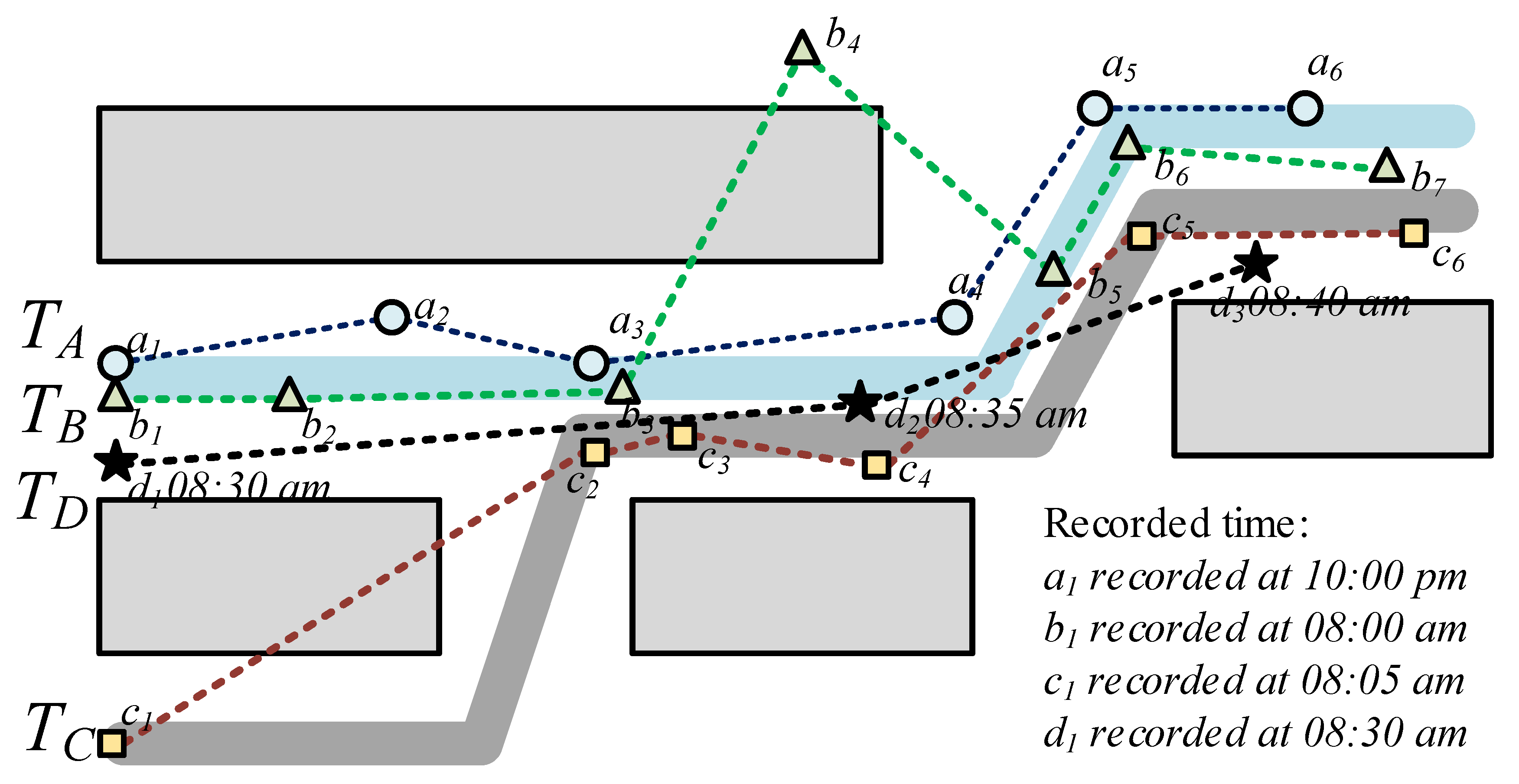
Figure 2.
The overall framework of multi-aspect embedding for attribute-aware trajectories (MAEAT): Aspect component acquisition is depicted on the left, and the MAEAT with two aspects (K = 2) is shown on the right, where HMM denotes a hidden Markov model. Note that the MAEAT could also be used to model the on-road trajectory case with temporal and spatial aspects as shown in Figure 1.

Figure 3.
A running example: A road network with GPS points shown on the left and its corresponding hidden Markov model (HMM) for the map-matching algorithm shown on the right.
Figure 3.
A running example: A road network with GPS points shown on the left and its corresponding hidden Markov model (HMM) for the map-matching algorithm shown on the right.
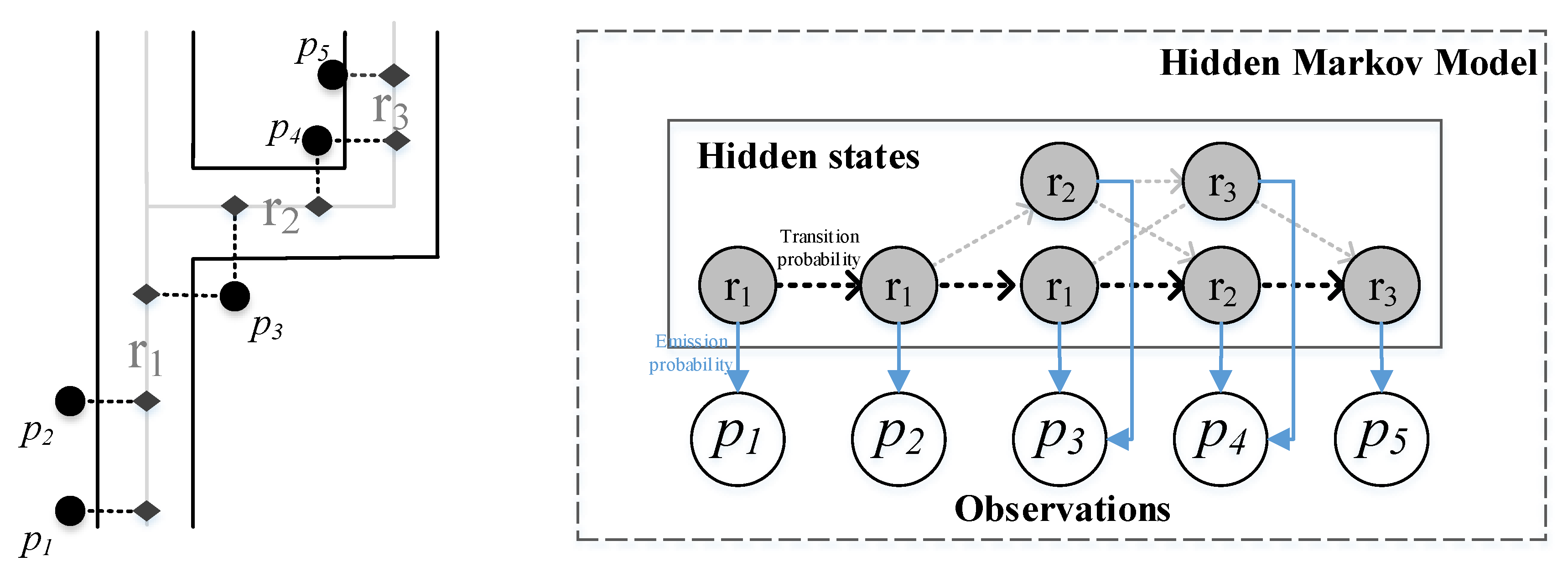
Figure 4.
Temporal clustering.
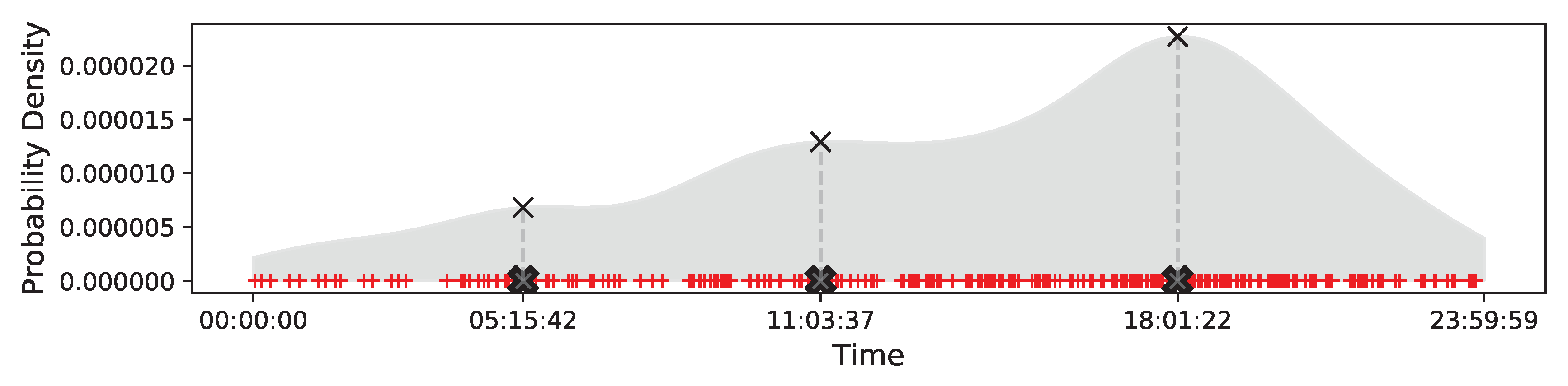
Figure 5.
K-nearest neighbour query: We use circle (◯) and cross (×) symbols represent the start and end points of the trajectories, respectively. Note that the rank number indicates how the retrieved trajectory is similar to the query, namely the similarity score between the query and trajectories Rank 1 > Rank 2 Rank 5.

Figure 6.
Efficiency Comparison. The run times during the training phase of model-based methods are shown on the left figure (a), while the similarity computation times between trajectories of the compared methods are shown on the right figure (b). Note that we denote the run times of Euclidean and Cosine computations by E-X and C-X, respectively, where X is the embedding vector size, on the right figure.
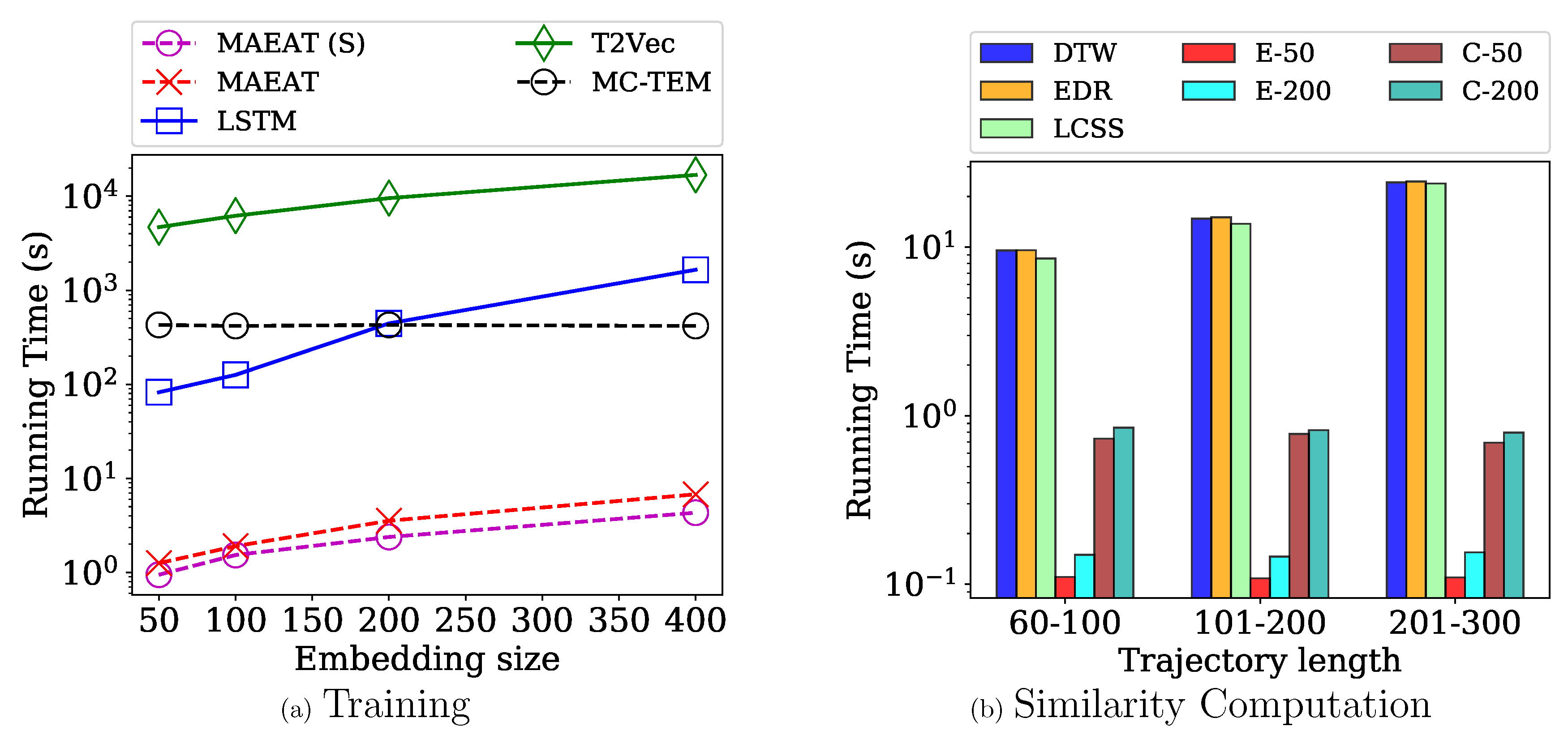
Figure 7.
K-nearest neighbour query performed by MAEAT with different .

Table 1.
Notations and descriptions.
| Notation | Description |
|---|---|
| T | trajectory T |
| the length of trajectory T | |
| the state i of a trajectory | |
| the set of attributes of state i ( = ) | |
| the number of attributes of state i ( = ) | |
| , | j-th attribute of state i in sets , |
| K-aspect trajectory corresponding to trajectory T | |
| K | the number of aspects considered in the model |
| K-aspect Sequence corresponding to | |
| the set of K discrete tokens corresponding to | |
| the discrete token reflecting the attribute | |
| the trajectory database | |
| v | an embedding vector |
| the embedding vectors for discrete token , trajectory T | |
| b-th embedding vector of a-th aspect | |
| tuning parameter that weights the importance of the aspect a | |
| learning rate |
Table 2.
Dataset statistics.
| Dataset | i5sim | i5sim3 | cross | cross2 | cross3 | Porto |
|---|---|---|---|---|---|---|
| #Trajectories | 800 | 1600 | 1900 | 1900 | 1900 | 5000 |
| #Points | 13,745 | 54,011 | 24,420 | 24,420 | 24,420 | 803,717 |
| #Clusters | 8 | 16 | 19 | 13 | 39 | N/A |
| Average Length | 17 | 34 | 13 | 13 | 13 | 161 |
Table 3.
Clustering quality comparison. We highlight the best performances in bold face.
| Compared Method | i5sim | i5sim3 | cross | cross2 | cross3 | |||||
|---|---|---|---|---|---|---|---|---|---|---|
| Purity | ARI | Purity | ARI | Purity | ARI | Purity | ARI | Purity | ARI | |
| Dynamic time warping (DTW) | 1.0 | 1.0 | 1.0 | 1.0 | 0.974 | 0.955 | 1.0 | 1.0 | 0.402 | 0.320 |
| Edit distance on real sequence (EDR) | 1.0 | 1.0 | 0.999 | 0.997 | 0.610 | 0.518 | 0.692 | 0.564 | 0.4 | 0.339 |
| Longest common subsequence (LCSS) | 1.0 | 1.0 | 0.993 | 0.985 | 0.985 | 0.969 | 0.797 | 0.689 | 0.392 | 0.311 |
| DISON | 1.0 | 1.0 | 0.691 | 0.738 | 0.687 | 0.726 | 0.797 | 0.453 | 0.225 | 0.453 |
| Encoder-Decoder (Recurrent neural network: RNN) | 1.0 | 1.0 | 0.864 | 0.839 | 0.026 | 0.152 | 0.192 | 0.023 | 0.116 | 0.014 |
| Encoder-Decoder (Gated recurrent unit: GRU) | 1.0 | 1.0 | 0.996 | 0.991 | 0.521 | 0.385 | 0.598 | 0.433 | 0.332 | 0.264 |
| Encoder-Decoder (Long-short term memory: LSTM) | 1.0 | 1.0 | 0.997 | 0.995 | 0.669 | 0.604 | 0.821 | 0.752 | 0.397 | 0.342 |
| T2Vec | 1.0 | 1.0 | 0.519 | 0.539 | 0.779 | 0.718 | 0.622 | 0.524 | 0.252 | 0.191 |
| MC-TEM | 1.0 | 1.0 | 0.574 | 0.542 | 0.861 | 0.819 | 0.927 | 0.919 | 0.751 | 0.680 |
| MAEAT(S) | 1.0 | 1.0 | 1.0 | 1.0 | 0.706 | 0.739 | 1.0 | 1.0 | 0.407 | 0.403 |
| MAEAT | - | - | - | - | - | - | - | - | 0.982 | 0.963 |
© 2019 by the authors. Licensee MDPI, Basel, Switzerland. This article is an open access article distributed under the terms and conditions of the Creative Commons Attribution (CC BY) license (http://creativecommons.org/licenses/by/4.0/).
Share and Cite
MDPI and ACS Style
Boonchoo, T.; Ao, X.; He, Q. Multi-Aspect Embedding for Attribute-Aware Trajectories. Symmetry 2019, 11, 1149. https://doi.org/10.3390/sym11091149
AMA Style
Boonchoo T, Ao X, He Q. Multi-Aspect Embedding for Attribute-Aware Trajectories. Symmetry. 2019; 11(9):1149. https://doi.org/10.3390/sym11091149
Chicago/Turabian StyleBoonchoo, Thapana, Xiang Ao, and Qing He. 2019. "Multi-Aspect Embedding for Attribute-Aware Trajectories" Symmetry 11, no. 9: 1149. https://doi.org/10.3390/sym11091149
Note that from the first issue of 2016, this journal uses article numbers instead of page numbers. See further details here.