Article

Monte Carlo Study of Rubber Elasticity on the Basis of Finsler Geometry Modeling †

1
National Institute of Technology (KOSEN), Sendai College, 48 Nodayama, Medeshima-Shiote, Natori-shi, Miyagi 981-1239, Japan
2
ELyTMaX UMI 3757, CNRS-Universite de Lyon, Tohoku University, International Joint Unit, Tohoku University, 2-1-1 Katahira, Aoba-ku, Sendai 980-8577, Japan
3
Frontier Research Institute for Interdisciplinary Sciences (FRIS), Tohoku University, 6-3 Aoba Aramaki, Aoba-ku, Sendai 980-8578, Japan
4
Materials Engineering and Science (MATEIS), CNRS, INSA Lyon UMR 5510, Université de Lyon Batiment B. Pascal, Avenue Jean Capelle, 69621 Villeurbanne, CEDEX, France
5
Institute of Fluid Science (IFS), Tohoku University, 2-1-1 Katahira, Aoba-ku, Sendai 980-0812, Japan
*
Author to whom correspondence should be addressed.
This work is supported in part by JSPS KAKENHI Grant No. JP17K05149 and the Collaborative Research Project of the Institute of Fluid Science, Tohoku University.
Symmetry 2019, 11(9), 1124; https://doi.org/10.3390/sym11091124
Submission received: 30 June 2019 / Revised: 12 August 2019 / Accepted: 17 August 2019 / Published: 4 September 2019

Abstract

:
Configurations of the polymer state in rubbers, such as so-called isotropic (random) and anisotropic (almost aligned) states, are symmetric/asymmetric under space rotations. In this paper, we present numerical data obtained by Monte Carlo simulations of a model for rubber formulations to compare these predictions with the reported experimental stress–strain curves. The model is defined by extending the two-dimensional surface model of Helfrich–Polyakov based on the Finsler geometry description. In the Finsler geometry model, the directional degree of freedom σ of the polymers and the polymer position r are assumed to be the dynamical variables, and these two variables play an important role in the modeling of rubber elasticity. We find that the simulated stresses τ sim are in good agreement with the reported experimental stresses τ exp for large strains of up to 1200 % . It should be emphasized that the stress–strain curves are directly calculated from the Finsler geometry model Hamiltonian and its partition function, and this technique is in sharp contrast to the standard technique in which affine deformation is assumed. It is also shown that the obtained results are qualitatively consistent with the experimental data as influenced by strain-induced crystallization and the presence of fillers, though the real strain-induced crystallization is a time-dependent phenomenon in general.

1. Introduction

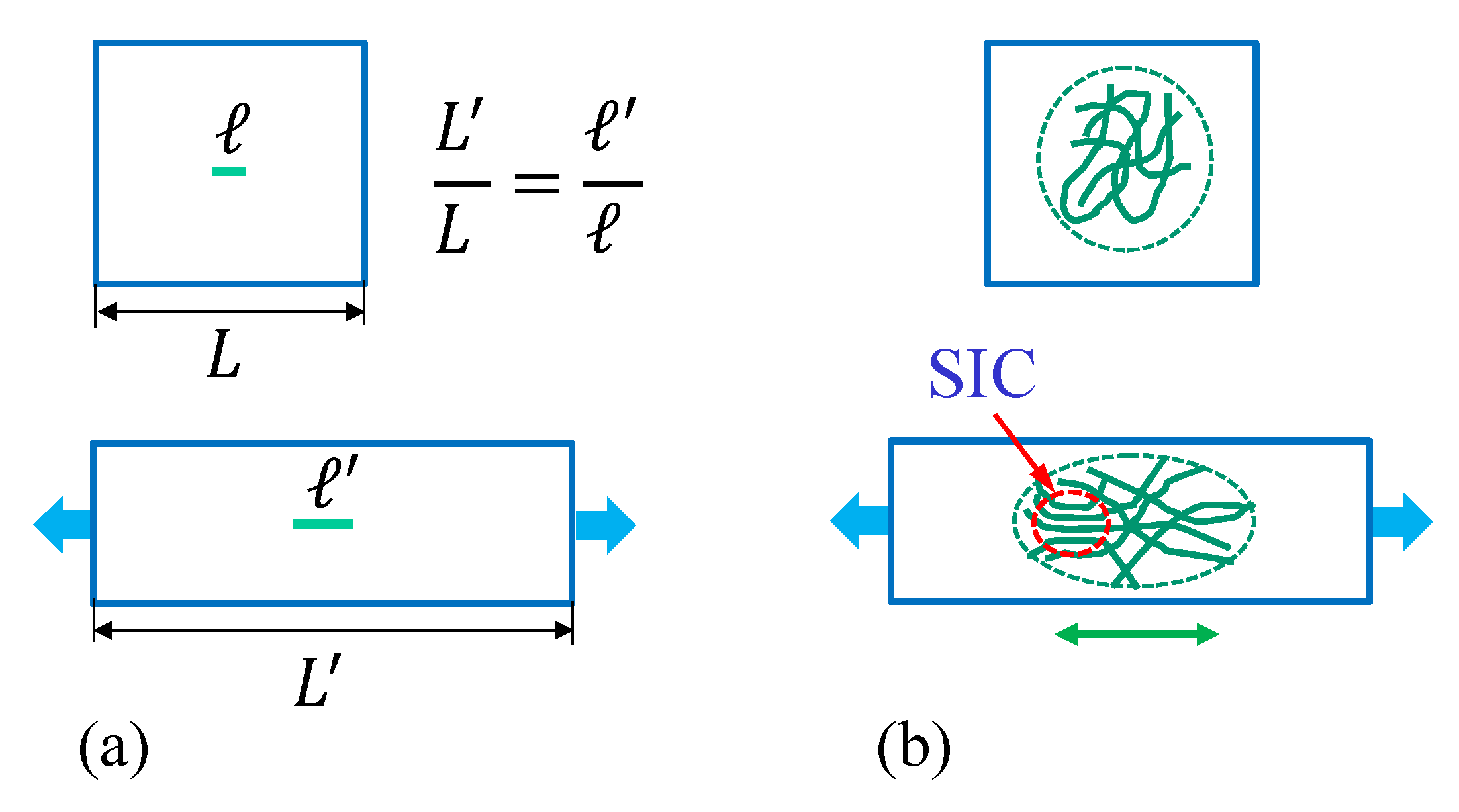
Rubbers such as natural rubber are well known to support large recoverable strains in the elastic deformation process of stretching/recovery (Figure 1a,b). An important characteristic of natural rubber is that it crystallizes during the stretching process, which is called strain-induced crystallization [1,2,3,4]. This strain-induced crystallization slows down crack propagation and therefore improves the natural rubber tearing properties. Other than the strain-induced crystallization, so-called fillers also play an important role in determining the mechanical properties and inducing hysteresis behavior in the stress–strain curve.
The stress–strain curve of rubbers is generally highly nonlinear and has a plateau-like structure in the intermediate strain region. One of the well-studied theories describing such a stress–strain curve is so-called affine network theory [5,6,7,8,9,10]. In this theory, the basic assumption is that the probability distribution of the polymer length follows a Gaussian distribution. In addition, the affine transformation is simply assumed in this theory for polymer elongation using the deformation tensor. In this framework, the free energy of the network is obtained, and the stress–strain curve becomes calculable [11,12,13,14,15,16]. In addition to this basic theory, many variations have been proposed, and, consequently, the stress–strain curves are well understood [17,18,19,20]. Other than the properties of the extended and highly nonlinear behavior of the stress–strain curves, it is also well known that the temperature of rubbers increases in the adiabatic extension process. This property characteristic of rubbers is called entropy elasticity, which is reflected in the stress being proportional to the temperature. This aspect is also well represented in the Gaussian chain model for polymers [5,6,7,8].
However, the above-mentioned Gaussian distribution is established only in a freely joined polymer chain by the central limit theorem, where neither the effect of entanglement nor many-body interaction is implemented. Moreover, the network theories are constructed under the assumption of the aforementioned affine deformation for all distances. This assumption is equivalent to the fact that rubbers are considered an ideal network with no microscopic interaction between segments [21]. As a consequence, rubbers are, in some sense, considered a continuum elastic material, in which there is no difference between the microscopic and macroscopic strains (Figure 2a). The problem is that it is still unclear why the assumption of affine deformation is satisfied or reasonable. In fact, it is well known and accepted that rubbers are crosslinked and not always uniform, and, moreover, strain-induced crystallization clearly makes the mechanical properties anisotropic (Figure 2b). It is also experimentally well known that entropy elasticity has a dominant contribution to the elasticity; however, the microscopic origin of this entropy elasticity is still quantitatively unclear. Thus, despite the fact that the study of rubber elasticity has a long history, the understanding of its basic properties is still unsatisfactory.
Therefore, it is interesting to study rubbers using mathematical theory without assuming affine deformation. For this purpose, we consider the Finsler geometry model to be a suitable technique [22] because the Finsler geometry model allows us to avoid complicated interactions and find another route, which is physically/mathematically transparent, to obtain the same results. Indeed, the above-mentioned plateau-like structure in the stress–strain curve can be reproduced by the Finsler geometry modeling technique in the case of a liquid crystal elastomer [23] and the J-shaped stress–strain curve of soft biological materials [24,25]. In this paper, we show that experimentally observed and reported that stress–strain curves of rubbers are reproducible by the Finsler geometry modeling technique without the affine deformation assumption [26]. Moreover, it is also shown that the stress formula is consistent with the entropy elasticity, in which the stress is proportional to the temperature.
In the Finsler geometry model, the internal directional degree of freedom σ is assumed to define the Finsler length inside the material. The Finsler length is not a real distance but is used to define the interaction energy, such as the Gaussian bond potential, which consequently becomes anisotropic. In the case of liquid crystal elastomer, the director field is assigned to σ and is assumed to have a nonpolar interaction governed by the so-called Lebwohl–Lasher potential [27]. For soft biological materials such as skin and arteries, the variable σ corresponds to the direction of the collagen fibers and also exhibits nonpolar interaction [24,25]. By considering the role of σ in these materials, it is natural to assume that the direction of the polymer chains corresponds to σ in the Finsler geometry model for rubbers, and the interaction between the variables σ is assumed to be the Lebwohl–Lasher potential.
This paper is organized as follows: in Section 2, we present the Hamiltonians of the three-dimensional (3D) and two-dimensional (2D) Finsler geometry models, the Monte Carlo technique, and the calculation formula for the frame tension. Readers who are not interested in these technical details can skip Section 2 and go to Section 3, where the Monte Carlo results, reported experimental data, and snapshots are presented. Finally, in Section 4, we summarize the results. In Appendix A and Appendix B, the detailed information of the discrete expressions of the tensile energies of the 2D and 3D models is described. The expression of the 2D bending energy is also described in Appendix B.

2. Models and Simulation Technique

2.1. Lattices and the Monte Carlo Technique

First of all, we emphasize that our model is a statistical mechanical one, and, hence, it is applicable to equilibrium properties of materials. For this reason, only stress–strain data observed in sufficiently long time measurements are targeted in this paper.
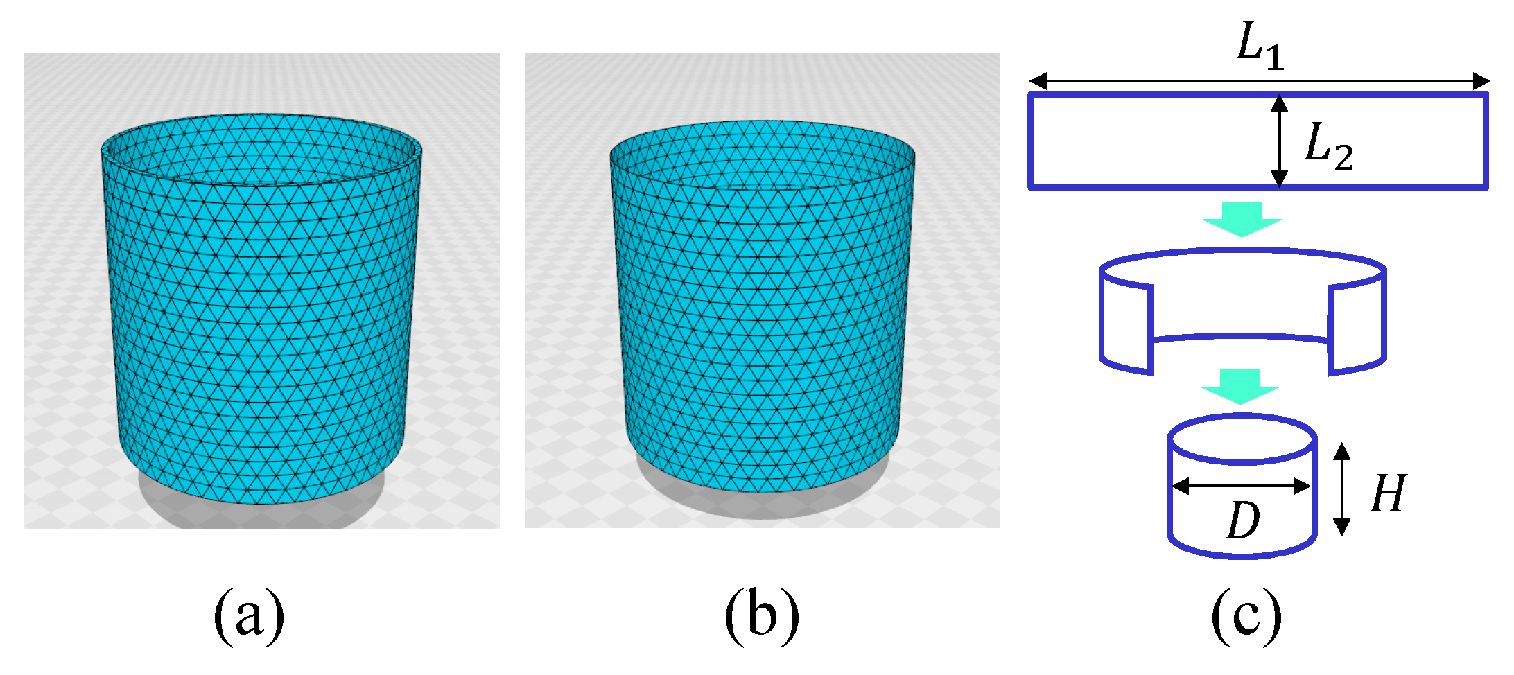
The Hamiltonians, which are introduced in the following subsections, are discretized on 3D and 2D lattices, which are composed of tetrahedrons (Figure 3a) and triangles (Figure 3b), respectively [25]. The cylinder in Figure 3a is a “thick” surface, which is composed of tetrahedrons, while the 2D cylinder in Figure 3b is a “real” surface. The ”thick” surface is a 3D lattice constructed by 3D tetrahedrons; however, the thickness is very small compared to the diameter or the height of the cylinder. In this sense, we call this 3D lattice a “thick” surface. The size of the 3D lattice in Figure 3a is given by ( N , N B , N T , N tet ) = ( 2226 , 10812 , 14946 , 6360 ) , where N, N B , N T , and N tet are the total number of vertices, bonds, triangles, and tetrahedrons, respectively. The topological constraint N N B + N T N tet = 0 , which is the Euler number, can be used to check whether the discretization is accurate or not. The size of the 2D lattice in Figure 3b is given by ( N , N B , N T ) = ( 1134 , 3294 , 2162 ) , where N, N B , and N T are the same as above. The Euler number for a 2D cylindrical lattice is given by N N B + N T = 2 , which is satisfied for the cylinder in Figure 3b. We use relatively small lattices in Figure 3a,b so that the lattice structure is clearly visible, and these lattices are considerably smaller than those used for the simulations.
The reason why we use such cylindrical lattices is that the cylindrical surface is suitable for a frame tension formula [28,29,30]. The frame tension is calculated on the surfaces spanning a fixed frame, which we call the boundary frame. For the calculation of the frame tension, it is better to remove a couple of unnecessary boundaries from the square boundary, as in Figure 3c. The calculation technique for the frame tension is presented in the separate subsection.
The 2D cylinder is constructed as follows: let a be the edge length of the regular triangle, and let ( L 1 , L 2 ) be the total number of divisions along the horizontal ( L 1 ) and vertical ( L 2 ) directions of the plate in Figure 3c; then, the height H and the diameter D of the cylinder are given by ( H , D ) = ( L 1 a / π , L 2 a 3 / 2 ) . In this paper, we use lattices of H = D ; then, we have L 1 = 3 L 2 π / 2 , and, therefore, H ( = D ) is given by a single integer L ( = L 2 ) such that
H = D = ( 3 / 2 ) L a .
For the 2D lattice in Figure 3b, we fix L to L = 20 . The lattice spacing a is fixed to a = 1 henceforth [31], and a is used later when the results are compared with the experimental data.
The 3D thick cylinder shown in Figure 3a is also generated to satisfy H = D by the Netgen Mesh Generator [32]. In this thick cylinder, the thickness is negligible compared to D, and, hence, the internal diameter and external diameter are simply expressed by D. We should note that there is no internal vertex between these outer and inner surfaces of the 3D lattice in Figure 3a, and the 3D lattice for the simulations also has vertices only on the outer and inner surfaces.
The calculation technique of the tensile stress, which is described later in detail, is based on the formula for the surface or frame tension. The frame tension is initially defined on two-dimensional surfaces. This is the reason why the 2D lattice is used to calculate the stress–strain curves. Moreover, as mentioned above, the 3D lattice is a thick cylinder and is considered to be a surface. Indeed, the frame tension formula, which is always applied in two-dimensional cases, is applied to the results obtained by the 3D lattice simulations.

2.2. 3D Model

The thick cylinder, such as the one in Figure 3a, is composed of tetrahedrons; therefore, a 3D model is necessary to use these thick cylinders. The continuous expression of the tensile energy function is given by a linear combination of the Gaussian bond potential S 1 and its simple quadratic extension S 2 such that
S = b S 1 + c S 2 , S 1 = g d 3 x g a b r x a · r x b , S 2 = g d 3 x g a b r x a · r x b 2 ,
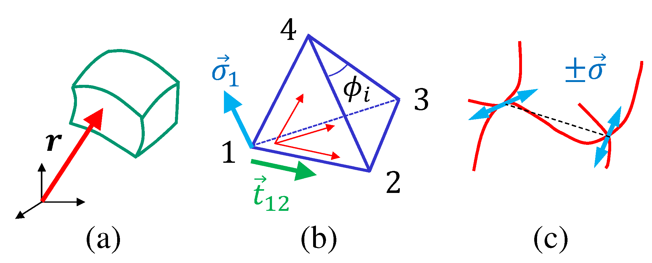
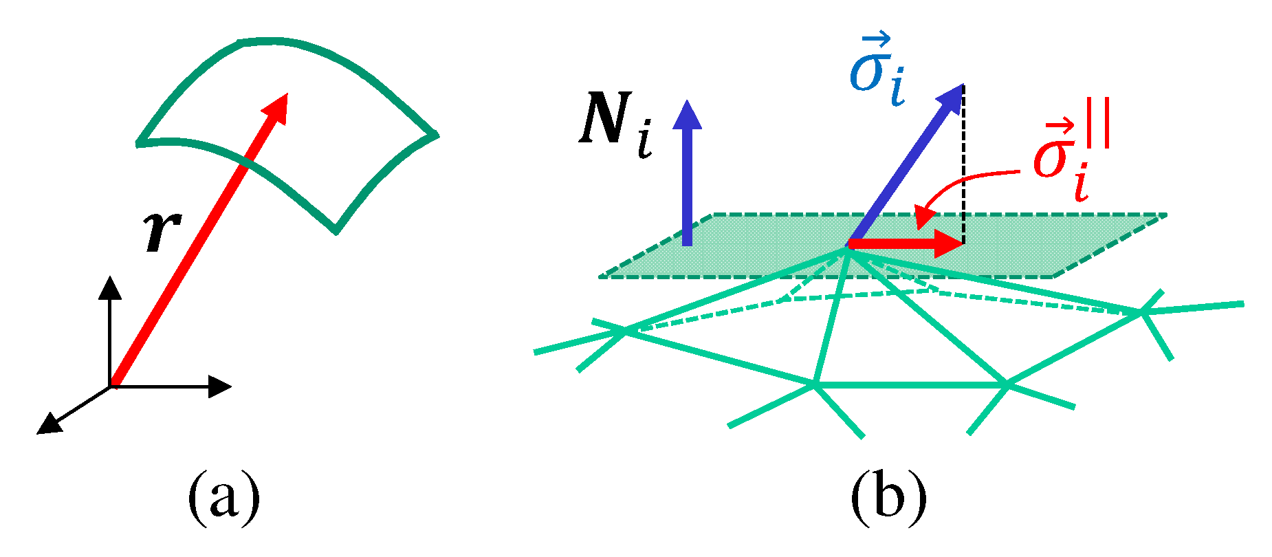
where r is a three-dimensional vector r = ( X , Y , Z ) ( R 3 ) and the elements X , Y , Z are functions of ( x 1 , x 2 , x 3 ) . Thus, the vector r represents the material position (Figure 4a), and this position vector r is also considered to be a mapping from a three-dimensional parameter space M to the three-dimensional Euclidean space R 3 such that r : M ( x 1 , x 2 , x 3 ) X ( x 1 , x 2 , x 3 ) , Y ( x 1 , x 2 , x 3 ) , Z ( x 1 , x 2 , x 3 ) R 3 . The 3 × 3 matrix g a b is the inverse of a metric tensor g a b on M, and g ( = det g a b ) is its determinant. Since the coefficient b is called the microscopic surface tension in the case in which M is a two-dimensional space, we call these b and c parameters tension coefficients.
Before discussing the discretization of S 1 and S 2 , we have to introduce the discrete Finsler metric
g a b = 1 / v 12 2 0 0 0 1 / v 13 2 0 0 0 1 / v 14 2 ,
where v i j is the Finsler length [22,33,34,35,36] given by
v i j = 1 | t i j · σ i | 2 + v 0 , t i j = i j / i j , i j = r j r i .
Note that v i j is different from v i j = | t i j · σ i | + v 0 used in Ref. [23]. The symbol t i j is a unit tangential vector along the edge or bond i j (see Figure 4b), and the variable σ i ( S 2 : unit sphere ) represents the direction of the polymer [37] (Figure 4c). The polymer directions are also coarse-grained by σ i . The parameter v 0 is introduced as a cutoff to avoid the divergence of the elements of g a b and is fixed to v 0 = 0.001 in this paper. This value is sufficiently small, and, therefore, the final results are independent of the small variation of v 0 around v 0 = 0.001 .
The discretization of these continuous functions S 1 and S 2 is described in Appendix A. By including several additional terms, the final form of the discrete Hamiltonian is given by
S ( r , σ ) = λ S 0 ( σ ) + b S 1 ( r , σ ) + c S 2 ( r , σ ) + κ S 3 ( r ) + U 3 D ( r ) + U B ,
where
S 0 ( σ ) = 1 2 i j 1 3 ( σ i · σ j ) 2 , S 1 = i j Γ i j i j 2 , Γ i j = 1 N ¯ tet γ i j ( tet ) , S 2 ( σ ) = i j Γ i j ( 1 ) i j 4 + i j , k l Γ i j , k l ( 2 ) i j 2 k l 2 , S 3 ( r ) = i 1 cos ( ϕ i π / 3 ) ,
and
U 3 D ( r ) = tet U 3 D ( tet ) , U 3 D ( tet ) = 0 ( Vol ( tet ) > 0 ) ( otherwise ) , U B = i boundary U B ( r i ) , U B ( r i ) = ( | z i H | > δ B or | z i | > δ B ) 0 ( otherwise ) .
The first term λ S 0 with the interaction coefficient λ represents the interaction between σ i and σ j , where i j denote the vertices connected by a bond. This S 0 is exactly the same as the Lebwohl–Lasher potential for liquid crystal molecules [27]. This term plays an important role in the Finsler geometry model because the variable σ in Equation (4) is used to define v i j and hence the elements of the Finsler metric in Equation (3). In the expression of S 1 , the coefficient N ¯ is defined by
N ¯ = 1 / N B i j n i j ,
where N B is the total number of bonds and n i j is the total number of tetrahedrons sharing the bond i j . Note that b Γ i j plays a role in the effective tension, in which the expression for the symbol γ i j is given in Appendix A. The symbols Γ i j ( 1 ) and Γ i j , k l ( 2 ) in S 2 are also given in Appendix A, and c Γ i j ( 1 ) and c Γ i j , k l ( 2 ) can also be understood as effective tensions corresponding to the quadratic terms of i j 4 and i j 2 k l 2 , respectively.
The fourth term κ S 3 is an energy for deformation of the tetrahedrons except simple swelling/shrinking, for which this term remains unchanged. In this expression of S 3 , the symbol ϕ i is an internal angle such as the one shown in Figure 4b, and i denotes the sum of all internal angles of the triangles. We call κ the bending rigidity because this term S 3 is considered to be an energy term corresponding to the bending energy in the 2D model, which is also described in the following subsection.
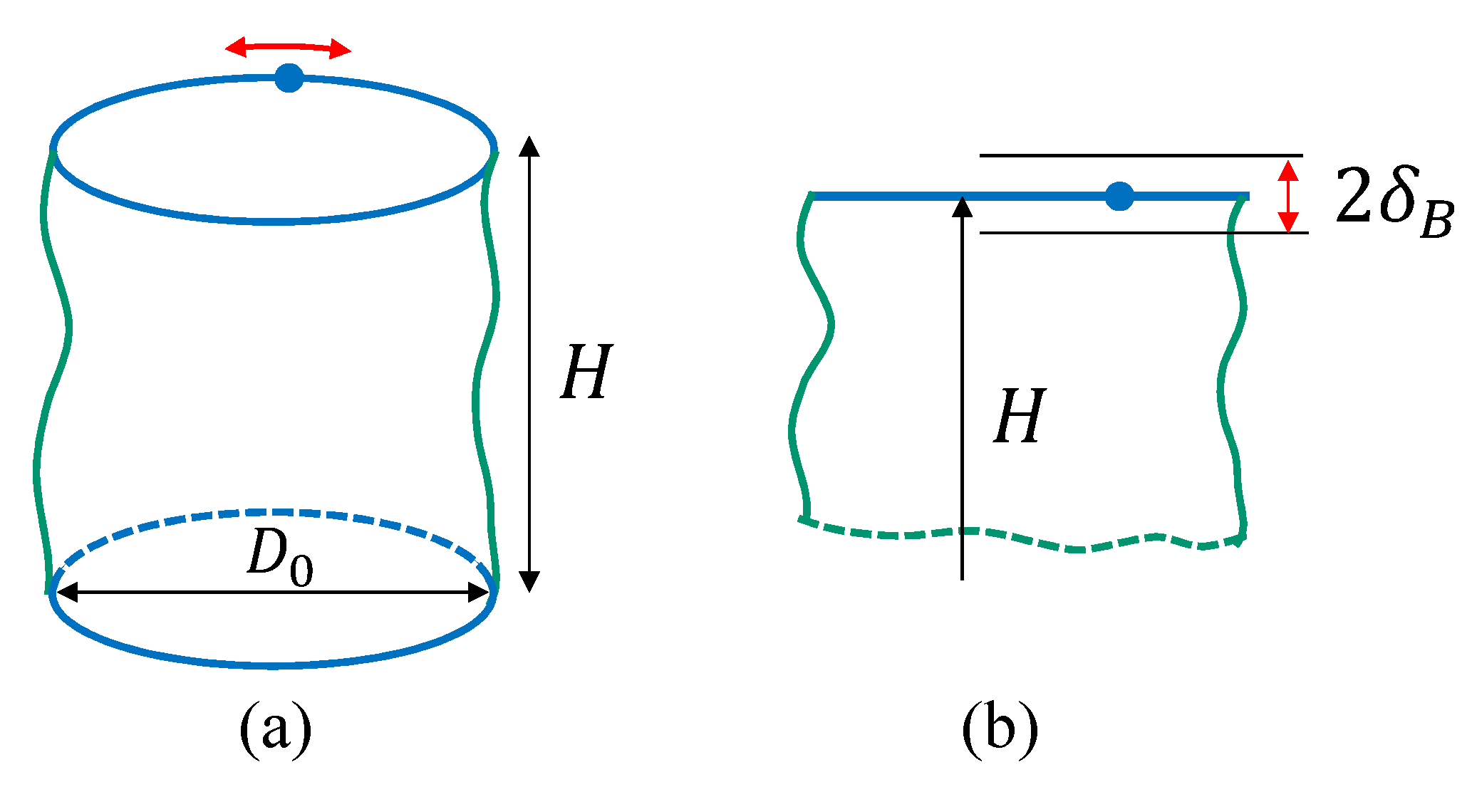
The fifth term U 3 D is a constraint potential such that the volume should not be negative for all tetrahedrons. The boundary vertices are allowed to fluctuate along the boundary circles of fixed diameter D 0 (Figure 5a), though this constraint is not written in the form of a mathematical expression. The final term U B is introduced for the boundary vertices. In this U B , the symbol δ B denotes a small distance above and below the boundary position (Figure 5b). Inside this gap 2 δ B , the boundary vertices are allowed to fluctuate not only along the boundary circle but also in the vertical direction. The small number δ B is given by the mean bond length of the initial lattice such that δ B = , and therefore δ B is negligible compared to H for sufficiently large N. The reason why this δ B is introduced for the boundary vertices is that the variable σ i at the boundary cannot be parallel to the boundary if the boundary circle is on a plane perpendicular to the z direction because v i j in Equation (4) makes 1 / v i j very large in this case.
To summarize the role of the parameters λ , b, c and κ intuitively, the first λ is a coefficient of the Lebwohl–Lasher potential, and, hence, this λ controls or reflects the alignment strength of the polymer directions just as in the case of liquid crystals. The coefficients b and c also control/reflect the strength of the response to external tensile forces, and, therefore, these can be called “tension coefficients”, as mentioned above. The parameter κ controls/reflects the resistance to external forces that deform the tetrahedron shape. This deformation includes that expected under the uniaxial tensile force, and therefore κ shares the same role with b and c in part.
The partition function is defined by
Z 3 D ( λ , b , c , κ ; H ) = σ i = 1 2 N 1 d r i i = 1 N 2 N 1 d r i exp 1 k B T S ( σ , r ) , ( k B T = 1 ) ,
where N 1 is the total number of boundary vertices on one of the two boundaries. The integrations i = 1 2 N 1 d r i and i = 1 N 2 N 1 d r i are one-dimensional and three-dimensional multiple integrations for the boundary vertices and the vertices inside the boundaries, respectively. In the simulations, the coefficient k B T in Equation (9) is fixed to k B T = 1 , where k B is the Boltzmann constant and T is the absolute temperature. In this simulation unit, the parameters λ , b, c, and κ have values in the unit of k B T . The explicit relation between this simulation unit and the physical unit is necessary for the calculation of the frame tension and will be described below.

2.3. 2D Model

In this subsection, we introduce a 2D model, which is also similar to the 2D model for soft biological materials in Refs. [38,39,40,41,42,43,44,45]. The 2D surface model is an extension of the Doi–Edwards model for a 1D polymer [46], and, therefore, the 2D Finsler geometry model as well as the 3D Finsler geometry model is considered an extension of this 1D polymer model. The continuous form of the Hamiltonian is given by
S = b S 1 + c S 2 + κ S 3 , S 1 = g d 2 x g a b r x a · r x b , S 2 = g d 2 x g a b r x a · r x b 2 , S 3 = 1 2 g d 2 x g a b n x a · n x b .
The first and second terms S 1 and S 2 , respectively, are identical to those in the 3D model in Equation (2) except that the parameter space M is a two-dimensional surface in this 2D model. The symbol r is now considered to be a mapping from the two-dimensional space M to R 3 . As a consequence, the integration changes to the two-dimensional case g d 2 x , and the metric tensor g a b also changes to a 2 × 2 matrix (Figure 6a). The third term S 3 is the standard bending energy for surface models, where n is a unit normal vector of the surface [38,39,40,41,42,43,44,45].
Note that this 2D model has no conformal invariance because the following condition is not always satisfied: S 3 is invariant under the conformal transformation g a b ( x ) g a b ( x ) = f ( x ) g a b ( x ) for any positive function f ( x ) [47]. Equivalently, it is clear that there exists a positive function f ( x ) such that S 3 ( g a b ( x ) ) S 3 ( g a b ( x ) ) with g a b ( x ) = f ( x ) g a b ( x ) .
The discrete Hamiltonian is given by
S ( σ , r ) = λ S 0 + b S 1 + c S 2 + κ S 3 + U B , S 0 ( σ ) = 3 / 2 i j σ i · σ j 2 , S 1 = i j γ i j i j 2 , S 2 = i j Γ i j ( 1 ) i j 4 + i j , k l Γ i j , k l ( 2 ) i j 2 k l 2 , S 3 = i j κ i j 1 n i · n j ,
which are now defined on the triangles. In the first term S 0 , the symbol σ i is defined by
σ i = σ i ( σ i · N i ) N i ,
where N i is a unit normal vector of the tangential plane at the vertex i (Figure 6b). The vector N i is defined by
N i = j ( i ) A j ( i ) n j ( i ) j ( i ) A j ( i ) n j ( i ) ,
where A j ( i ) and n j ( i ) denote the area and the unit normal vector of the triangle j ( i ) sharing the vertex i, respectively. The parameter σ i is the tangential component of σ i and has values “inside” the unit sphere S 2 in contrast to the original σ , which is on S 2 .
The information on the symbols γ i j , Γ i j ( 1 ) and Γ i j , k l ( 2 ) in S 1 and S 2 is given in Appendix B. The symbols κ i j in S 3 are also defined in Appendix B. The roles of parameters λ , b, c and κ are exactly the same as those in the 3D model except that κ in this 2D model represents the resistance to pure bending deformation.

2.4. Formula for the Frame Tension

In this subsection, we present the formula for the calculation of the frame tension τ [28]. The frame tension τ is calculated from the scale invariant property of the partition function Z ( { r } ) , where { r } denotes the integration variables, which is simply expressed by r henceforth [48]. Since Z is independent of the integration variables, we have Z ( α r ) = Z ( r ) for any scale parameter α ( > 0 ) [28]. It follows from this relation that
log Z ( α r ) α α = 1 = 0 .
By applying the scale change r α r to the Hamiltonians of both the 2D and 3D models, we have S 1 ( α r ) = α 2 S 1 ( r ) and S 2 ( α r ) = α 4 S 2 ( r ) . All other terms in the Hamiltonian S remain unchanged under this scale transformation. The integrations in Z are changed to i = 1 2 N 1 d ( α r i ) i = 1 N 2 N 1 d ( α r i ) = α 2 N 1 + 3 ( N 2 N 1 ) i = 1 2 N 1 d r i i = 1 N 2 N 1 d r i .
Here, we note that the height H of the 3D and 2D cylinders is fixed. As a result of this constraint, the projected area A p of the frame is fixed such that
A p = π D 0 H ,
where D 0 is the initial diameter of the cylinders. This A p depends only on H and is independent of the diameter D of the cylinders, where D is not always identical to D 0 because D fluctuates in general due to surface fluctuations. This A p originally comes from the area of the square boundary shown in the upper part of Figure 3c.
The important point to note here is that the integrations in Z are performed under the fixed A p . This constraint is expressed in the scaled partition function such that Z ( α r , A p ( α ) ) , where A p ( α ) denotes that A p is implicitly dependent on α , and this dependence is described by A p ( α ) = α 2 A p . Thus, replacing Z ( α r ) in Equation (14) by Z ( α r , A p ( α ) ) , we have
( 3 N 4 N 1 ) 2 b S 1 4 c S 2 + log Z A p A p α α = 1 = 0 .
To evaluate the final term, we assume that the free energy F ( A p ) for the surface with the projected area A p satisfies
F = τ A 0 A p d A , Z = exp F .
This is the definition of the macroscopic surface (or frame) tension τ . From this Z, the final term of Equation (16) is identified with 2 τ A p . Thus, we have
τ = 2 b S 1 + 4 c S 2 ( 3 N 4 N 1 ) 2 A p .
This is the formula for the calculation of the frame tension. From this formula, we also understand that the macroscopic quantity 2 A p τ corresponds to the microscopically defined quantity 2 b S 1 + 4 c S 2 ( 3 N 4 N 1 ) , which is given by a linear combination of the simulation data S 1 and S 2 .
We emphasize that τ should not be understood as a nominal stress because the frame tension τ in Equation (18) is a notion for two-dimensional surfaces and is calculated by fixing the frame over which the surface extends. There is no difference between the ”nominal” and ”true” tensions in τ because the frame tension is a notion for surfaces. The only constraint for the frame tension is whether the surface actually extends over the boundary frame or not. If the surface collapses and becomes a string-like object such as a surface that undergoes a necking phenomenon [26], the string-like object no longer spans the boundary frame, and, in this case, the free energy of such an object is clearly different from F in Equation (17). The frame tension can be defined only when the surface retains its two-dimensional structure. Therefore, we check whether the surfaces span the boundary frame or not by visualizing them as snapshots.
Here, we should note that the equilibrium extension process of the surface is qualitatively consistent with a prediction of the thermodynamics of rubbers, which are considered to comprise a set of chains with freely rotating links forming a three-dimensional network [5,6,7,8]. Let S and U be the entropy and internal energy of rubber, respectively, which is expanded from L to L + d L by an external force f. Since the volume change is negligible, we have T d S = d U f d L from the energy conservation law. From this expression, we have f = ( U / L ) T ( S / L ) . The problem is whether the conditions ( U / L ) > 0 and ( S / L ) < 0 are consistent with the Finsler geometry model or not. If one of these two is violated, then f can be negative. Thus, it is meaningful to check these conditions. First, the direction of σ in the Finsler geometry model is controlled not only by the coefficient λ of S 0 in Equation (6) or Equation (11) but also by mechanical elongation or stresses. Let us assume λ = 0 . If the surface of the model is expanded by the external force f, the configuration of σ changes from disordered states to ordered states and aligns along the direction of f if λ is sufficiently small, including the case λ = 0 . Thus, the entropy is expected to be decreased, and ( S / L ) < 0 is expected. Moreover, the energy λ S 0 remains zero because λ = 0 even when S 0 decreases by the change of σ from disordered to ordered. As a consequence, the internal energy U corresponding to λ S 0 + b S 1 + c S 2 + κ S 3 is increased for the extension process of rubbers because S 1 , S 2 and S 3 increase when the surface height H is increased. Therefore, from this increase in internal energy, we expect that ( U / L ) > 0 .

2.5. Physical Unit of the Frame Tension

In this subsection, we show the formula for the comparison of the calculated frame tension τ with the experimental stresses τ exp ( N / m 2 ) [23,24]. We should first note that the physical unit of the frame tension is given by ( N / m ) and is different from ( N / m 2 ) of the stress τ exp , and, moreover, the calculation of τ in Equation (18) is performed using the simulation unit, which is determined by k B T = 1 as described in Equation (9). Therefore, the simulation unit should be changed to the physical unit. This unit change is made possible by using the lattice spacing a and k B T , and we have the physical frame tension τ sim ( N / m 2 ) , which can be compared with τ exp . The lattice spacing a is introduced to represent the edge length of the triangle at the beginning of Equation (1), and this role of a remains unchanged at this stage even when it is used to change the unit of τ [31].
Note that the physical unit of τ in Equation (18) is ( 1 / m 2 ) if A p is replaced by A p a 2 because the numerator is of unit one. Thus, the first step to change the unit of τ from the simulation unit to the physical unit is to replace A p with A p a 2 , and, consequently, we have τ sim = 2 b S 1 + 4 c S 2 ( 3 N 4 N 1 ) / ( 2 A p a 2 ) ( 1 / m 2 ) . The unit of τ sim can be changed further from ( 1 / m 2 ) to ( N / m 2 ) by multiplying k B T / a ( N ) , and we finally obtain
τ sim = 2 b S 1 + 4 c S 2 ( 3 N 4 N 1 ) 2 A p k B T a 3 = τ k B T a 3 ( N / m 2 ) .
This τ sim can be compared with the experimentally observed stresses τ exp ( N / m 2 ) . The fact that τ sim is proportional to T is consistent with the entropy elasticity, although τ is obtained by temperature-independent Monte Carlo simulations. In this paper, T is fixed to room temperature to compare τ sim with the experimental data τ exp , and the expression of τ sim is given by
τ sim = 4 × 10 21 τ a 3 ( N / m 2 ) ,
where the lattice spacing a can be varied as a free parameter such that τ sim is equal to τ exp in the whole or a part of the strain domain. The only constraint for a is that a should be larger than the van der Waals distance. This aspect is also checked in detail.

2.6. Monte Carlo Simulations

The standard Metropolis technique is used to update the variables r and σ [49,50]. The variable r is changed to a new position r such that r = r + δ r with a small random vector δ r given by three uniform random numbers. This new position r is accepted with the probability Min [ 1 , exp ( δ S ) ] , where δ S = S ( r ) S ( r ) is the energy difference between the new ( r ) and old ( r ) configurations. Note that the coefficient 1 / k B T is suppressed in exp ( δ S ) because of the assumption k B T = 1 for the simulation unit. The small vector δ r is inside a sphere of radius r 0 , which is fixed so that the rate of acceptance of r is approximately equal to 50 % . This rate of acceptance mainly depends on the initial height H (Figure 5a) and the coefficient κ of S 3 ; it becomes smaller for larger H and larger κ . For the update of boundary vertices, r is constrained to have values on the circle of diameter D 0 and also inside the small gap 2 δ B (Figure 5a,b). The variable σ is also updated to σ using the three random numbers σ x , σ y , σ z ( [ 0.5 , 0.5 ] ) such that σ = ( σ x , σ y , σ z ) / σ y 2 + σ x 2 + σ z 2 . Consequently, σ has values on the unit sphere, and the rate of acceptance of σ is not controllable. The rate of acceptance of r and that of σ remain unchanged during the simulations.
The total number of vertices of the lattices for the simulations are N = 9762 and N = 10 , 584 for the 3D and 2D models, respectively. The initial height H 0 ( = D 0 ) is fixed such that the frame tension τ in Equation (18) vanishes; τ = 0 . This H 0 is used for the strain
ε = H H 0 1 , ( H 0 = D 0 )
and hence H 0 should be carefully evaluated before the start of production runs. The parameter H 0 depends on the parameters λ , b , c and κ in both the 3D and the 2D models.
The convergence speed of the simulation is relatively fast because the surface fluctuations are considerably suppressed by the boundary circles (see Figure 5a). The thermalization Monte Carlo sweep is 5 × 10 6 , and the physical quantities are calculated every 1000 Monte Carlo sweeps during 3 × 10 7 4 × 10 7 Monte Carlo sweeps after the thermalization terations in both the 2D and the 3D models.

3. Numerical Results

3.1. Stress–Strain Curve and the Order Parameter

In this subsection, we present the simulation data τ sim in Equation (20) and the order parameter M, which is defined by
M = 3 2 σ z 2 1 3 .
We obtain τ sim and M by varying the parameters λ , b, c and κ and compare τ sim with the reported experimental data τ exp . The main purpose is to find that the Finsler geometry model can produce τ sim comparable to τ exp , and it is also interesting to find the role of these parameters in the behavior of τ sim and M.
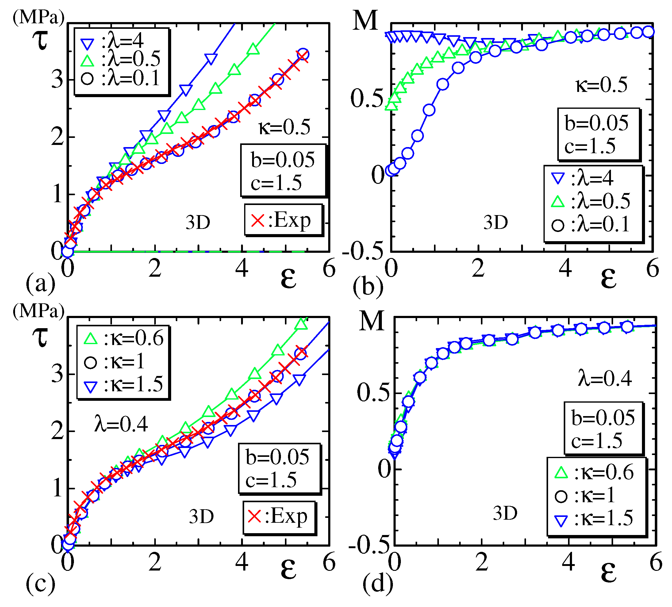
The parameter τ exp plotted in Figure 7a with the symbol (×) is the experimental (Exp) stress–strain data τ exp vs. ε of layered double hydroxide (LDH)-based elastomer nanocomposites reported in Ref. [51]. The τ exp of this nano-composite of ethylene propylene diene terpolymer (EPDM) and layered double hydroxide (LDH), denoted by EL10, shows a standard shape of the stress–strain curve of rubbers, where the number at the end of EL indicates the amount of LDH in phr (per hundred rubber). Indeed, the stress turns upwards for the large-strain region, and such an upturn of strain is known to be caused by both strain-induced crystallization and a failure or rupture phenomenon. Pradhan et al. analyzed the experimental data using a modified Mooney–Rivlin equation and found that this upturn of τ exp of the material EL10 is mainly due to the strain-induced crystallization [51].
The parameters b and c are fixed to b = 0.05 and c = 1.5 , respectively, in Figure 7a–d, which implies that the quadratic terms of in S 2 predominantly contribute to τ sim over the square term S 1 . In Figure 7a,b, different values of λ are tested: λ = 0.1 , 0.5 , 4 with fixed κ ( = 0.5 ) , while in Figure 7c,d, κ is varied as κ = 0.6 , 1 , 1.5 with fixed λ ( = 0.4 ) . The experimental data τ exp plotted in Figure 7c with the symbol (×) are the same as those in Figure 7a. As described in Section 2.5, the value of τ sim depends on the lattice spacing a. We choose a for τ sim in Figure 7a,c such that τ sim becomes almost identical to τ exp in the region of ε 1 approximately. The lattice spacing a assumed for τ sim is summarized in the following subsection.
We find from Figure 7a that the shape of τ sim is considerably dependent on the value of λ such that the slope of the curve decreases with decreasing λ in the intermediate region of ε . For large λ such as λ = 4 in Figure 7b, M is close to M 1 even at ε = 0 . This result implies that the variable σ aligns almost along the height direction, even for the small region of ε 0 . In contrast, for relatively smaller λ such as λ = 0.5 and λ = 0.1 , M decreases to M 0 for ε 0 , where σ is almost random. In the case of λ = 0.1 , M smoothly varies from M = 0 to M 1 , and, in this case, τ sim becomes close to τ exp . This result implies that the internal directional degrees of freedom of the polymer represented by σ play an important role in the highly nonlinear behavior of τ sim .
It is confirmed from Figure 7c that the slope can also be reduced by increasing κ . We also find from Figure 7d that the three Ms are almost identical to each other and vary from M 0.1 to M 1 with increasing ε . This variation of M is almost consistent with that of M in Figure 7b for λ = 0.1 , corresponding to the case of τ sim being close to τ exp in Figure 7a. This consistency in M is the reason that the corresponding stress–strain curve in Figure 7c is very close to the experimental data τ exp . However, the other two curves in Figure 7c deviate from the experimental data when κ increases/decreases from κ = 1 , even though M remains almost unchanged. From this finding, we understand that the stiffness of the material can also change the slope of the stress–strain curves without changing the internal structure of the material.
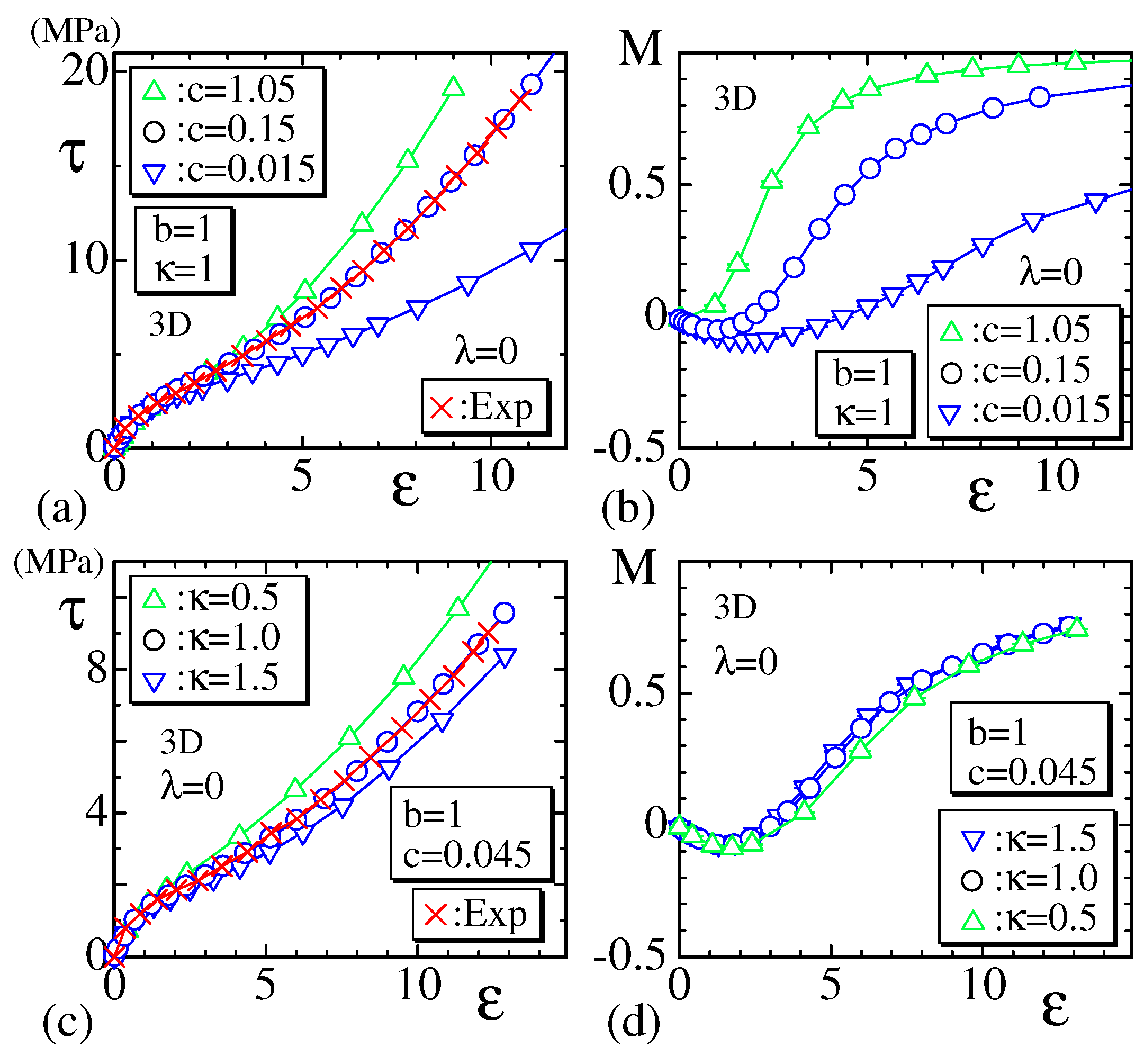
Next, we studied the experimental data of nanocomposites of carboxylated nitrile rubber (XNBR) and layered double hydroxide (LDH), denoted by XL10 and XL5 in Ref. [51], where the number at the end of XL indicates the amount of LDH in phr. The strain of the material is very large and extends up to 1200 % or more depending on the concentration of LDH, and upturns of the strain are also observed. The upturn of the strain is known to be partially due to the effect of strain-induced crystallization and also due to the presence of fillers, which lead to strain amplification. Therefore, in the large-strain region, the ideal chain assumption is no longer valid, and, hence, it is interesting to see whether the Finsler geometry model can produce such large-strain curves.
The simulation data plotted in Figure 8a,b are obtained by fixing the parameters b and c to b = 1 and c = 1.05 , 0.15 , 0.015 , respectively [52]. These combinations of b and c such that b ( = 1 ) c or b ( = 1 ) > c are in sharp contrast to those in Figure 7a–d, where b ( = 0.05 ) c ( = 1.5 ) . The parameter c ( κ ) is varied, and λ , b and κ (c) are fixed in Figure 8a,b (Figure 8c,d). The Exp data τ exp (×) in Figure 8a,c are for XL10 and XL5, respectively.
We find from Figure 8a (Figure 8c) that the slope of τ sim in the intermediate region of ε decreases with decreasing c (increasing κ ). From the behavior of τ sim in Figure 7a and Figure 8a, we find that the effect of reducing c on τ sim is almost the same as that of reducing λ . This result is also confirmed by comparing M in Figure 8b with the results plotted in Figure 7b. The only difference is that M in Figure 8b,d is not close to M 1 in the maximum ε region for sufficiently small c such as c = 0.015 and c = 0.045 . For a smaller region of c such as c = 0.0075 or less, M almost satisfies M 0 even for sufficiently large ε .
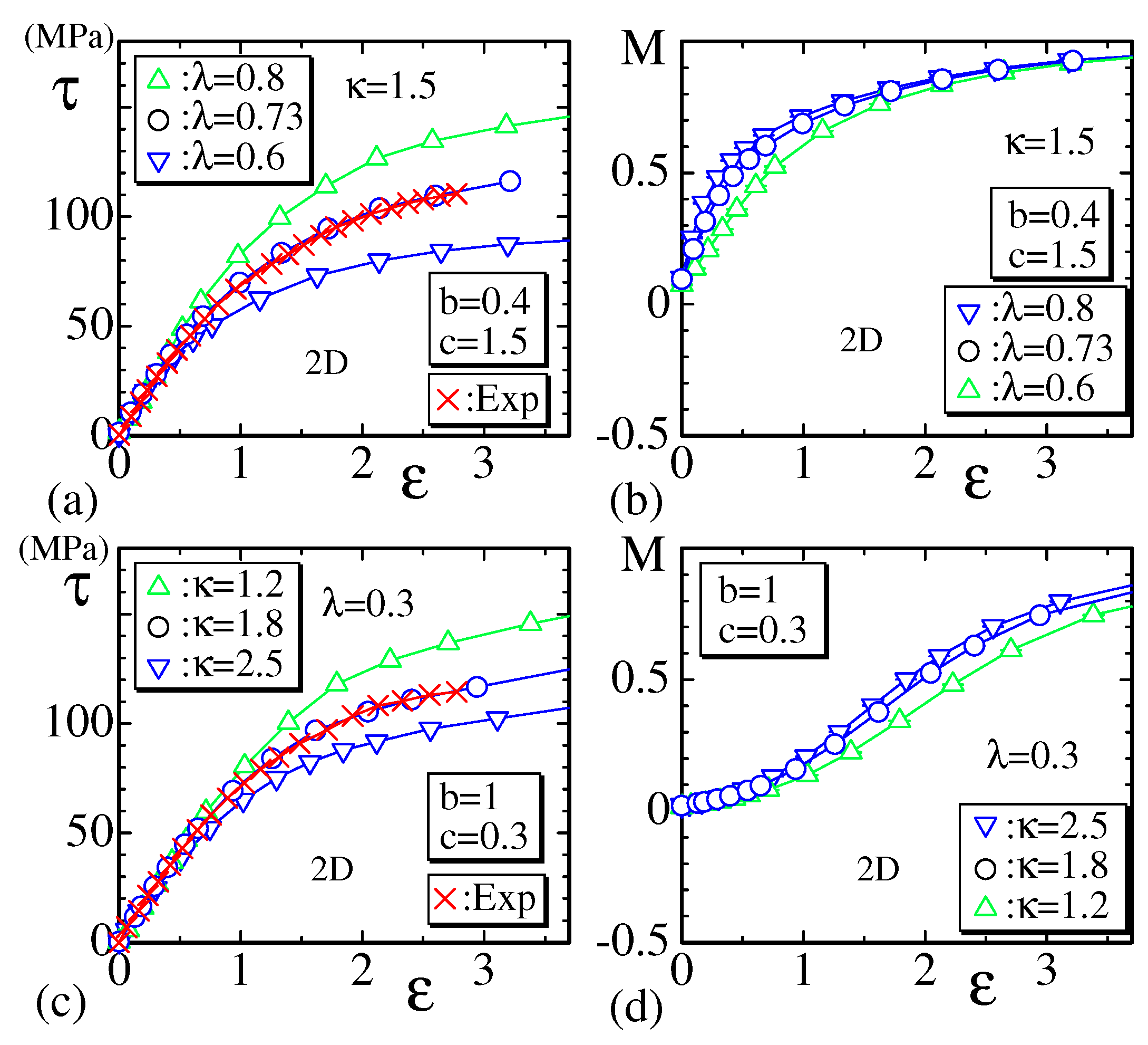
The 2D simulation data τ sim and M are shown with the experimental data τ exp of untreated cotton/vinyl ester composites reported in Ref. [53] in Figure 9a–d. In the experimental data for τ exp (×) in Figure 9a,c, no upturn is observed [54]. Therefore, the 2D model is suitable because the τ sim of the 2D model is always linear for the large-strain region. For τ sim in Figure 9a, λ is varied while b, c and κ are fixed to b = 0.4 , c = 1.5 and κ = 1.5 , respectively. The corresponding order parameters M in Figure 9b vary from M 0 to M 1 as ε increases from zero. This behavior is almost the same as that of the case λ = 0.1 in Figure 7b of the 3D model. We also confirm that M increases in the small-strain region if λ increases in the manner as M vs. ε in Figure 7b of the 3D model.
For τ sim in Figure 9c, κ is varied while λ , b and c are fixed to λ = 0.3 , b = 1 and c = 0.3 . It is also found from Figure 9d that M of the 2D model changes depending on κ , in contrast to the case of the 3D model in Figure 7d, where M remains unchanged against the variation in κ .
The arrangements of the parameters b and c in Figure 9a,b and Figure 9c,d are approximately close to those in Figure 7a,b and Figure 7c,d for the 3D model, respectively. We find that the slope of τ sim in the intermediate ε region of the 2D model increases with increasing λ , and this behavior is consistent with that of the 3D model shown in Figure 7a. We also find that the behavior of τ sim of the 2D model in Figure 9c against the variation in κ is consistent with that of the 3D model in Figure 7c.
To summarize, the experimental data τ exp without upturns in the large-strain region are reproducible by the 2D Finsler geometry model. It is also confirmed that there is almost no difference between the 2D and 3D models in the behavior of τ sim with respect to the variation of λ (Figure 7a and Figure 9a). This consistency in τ sim is not always trivial because a considerable difference is expected in the coefficients γ i j , Γ i j ( 1 ) and Γ i j , i k ( 2 ) in Equations (A4) and (A5) for the 3D model and those in Equation (A7) for the 2D model, as discussed in the final part of Appendix B.
Finally, in this subsection, we comment on the uniqueness of the combination of the input parameters. The problem is whether the parameters λ , b, c and κ are uniquely determined for a given stress–strain curve. Based on many simulations with a variety of input parameters, our observation is that there are at least two different combinations of parameters such that the stress–strain curves are almost the same. For example, in the 2D model, the stress–strain curves of ( λ , b , c , κ ) = ( 0.73 , 0.4 , 1 , 1.5 ) and ( λ , b , c , κ ) = ( 0.3 , 1 , 0.3 , 1.8 ) are almost identical. The first parameter set is used in Figure 9a,b. In the case of the 3D model, the results are almost the same for ( λ , b , c , κ ) = ( 0.1 , 0.05 , 1.5 , 0.5 ) and ( λ , b , c , κ ) = ( 0.4 , 0.05 , 1.5 , 1 ) , where the first one is used in Figure 7a,b. In the 2D and 3D models, the order parameters M are also relatively close to but slightly different from each other for the two different parameter sets. This difference of M mainly comes from the difference in λ , and it also implies a difference of the internal structure corresponding to the polymer direction.

3.2. Simulations for Strain-Induced Crystallization

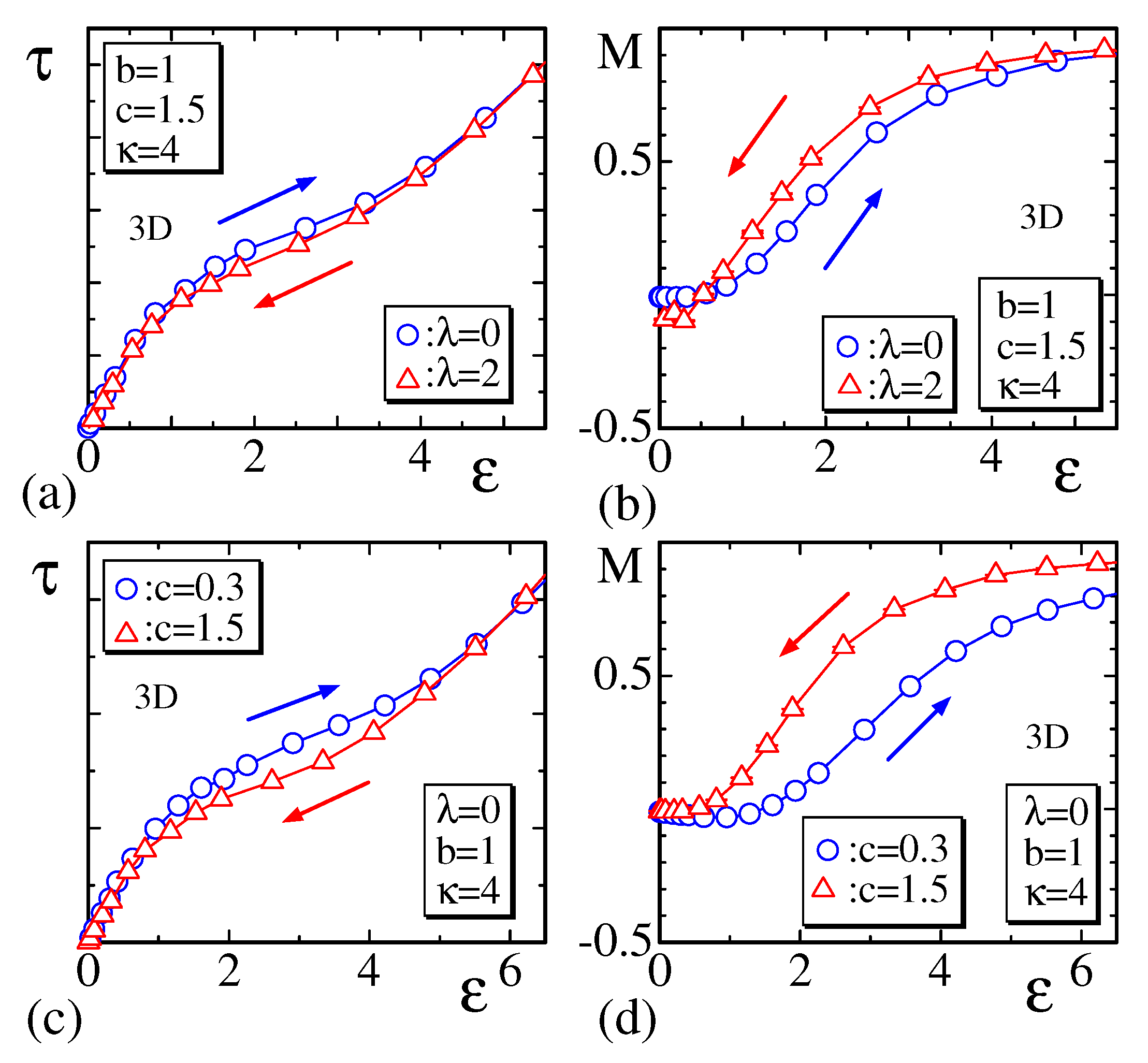
In the preceding subsection, we find that the dependence of τ sim on the variation of λ in the 2D model is consistent with that of the 3D model. This result indicates that the dependence of τ sim on the variation of λ is universal in the Finsler geometry model. Therefore, recalling that the crystallization ratio χ [1,2,3,4] is considered to be closely connected to M, it is interesting to see whether the response of τ and M against the change of λ in the 3D model is compatible with the values of τ exp and χ observed in the experiments on the extension/recovery processes. We have to emphasize that strain-induced crystallization is a time-dependent phenomenon, while the Monte Carlo results can represent only equilibrium properties; hence, the purpose of this subsection is simply to find whether the Monte Carlo results of the 3D model are compatible with the hysteresis behaviors in the experimental strain-induced crystallization data [1,2,3,4] (Figure 1b,c).
We plot two different stress–strain curves in Figure 10a obtained under b = 1 , c = 1.5 and κ = 4 . The difference of the curves comes from the difference of λ such that λ = 0 () and λ = 2 (), corresponding to the arrows pointing in opposite directions. The lattice spacing a is suitably chosen such that two curves of τ sim are identical to each other at ε 6 . The direction of the arrows in Figure 10a simply indicates that τ sim corresponds to the experimental extension/recovery process and does not mean that the simulations are so-called ”hysteresis simulations” [55]. In experiments, it is expected that the strain-induced crystallization is enhanced in the recovery process, and this enhancement is considered to be the origin of the reduction of the slope of the stress–strain curve in the intermediate region of ε . We find that the results in Figure 10a are compatible with this expectation because the increment of λ aligns with σ , which denotes the direction of the polymer chains. In Figure 10b, the order parameters M corresponding to τ sim in Figure 10a are plotted. We also find that the behavior of M is compatible with that of χ , which is expected to increase in the recovery process.
For another combination of parameters such as λ = 0 , b = 1 , κ = 4 , and with c = 0.3 , and c = 1.5 , we also obtain the hysteresis-like behavior of τ sim in Figure 10c. In this case, the difference in M is very large (Figure 10d), though the difference in τ sim in Figure 10c is not as large. In this case, the parameter c is changed for the stretching and recovery processes, while λ is fixed to λ = 0 . This result implies that the difference in the data () and () comes from the difference in the tensile energy c S 2 , which is directly connected to the mechanical properties of materials. In contrast, in the case of data in Figure 10a,b, the difference in the data () and () comes from the difference in λ S 0 , which is also connected to the mechanical properties of materials but indirectly. “Indirectly” implies that the tensile energies b S 1 and c S 2 can also be changed by the coefficients Γ i j , Γ i j ( 1 ) and Γ i j , k l ( 2 ) , which can also be changed by the orientation of σ in λ S 0 . Thus, from the data presented in Figure 10a–d, we find that the prediction of the Finsler geometry model is consistent with the strain-induced crystallization phenomenon.

3.3. Lattice Spacing and Snapshots

In this subsection, we first show the values of the lattice spacing a used in the calculations of τ sim in Table 1. From Equation (20), we have τ sim = 4 × 10 27 τ / a 3 ( MPa ) , which can be identified with τ exp ( MPa ) if a is suitably fixed. Equivalently, we have a = 4 τ / τ sim 1 / 3 × 10 9 ( m ) , where τ is the simulation data in simulation units and τ sim is the plotted data in Figure 7, Figure 8 and Figure 9 with the unit ( MPa ) . We find that all a in Table 1 are larger than the van der Waals distance ( 10 10 ( m ) ). Since the lattice spacing a corresponds to the bond length of tetrahedrons or triangles that form the projected surface and the bond length corresponds to the length of polymer chain segments, we find no problem if a is identified with the lattice spacing. Note that a corresponding to τ sim in Figure 10a,c is almost comparable with a for τ sim in Figure 7a and Figure 8a, respectively. For this reason, the values of a for τ sim in Figure 10a,c are not included in Table 1.
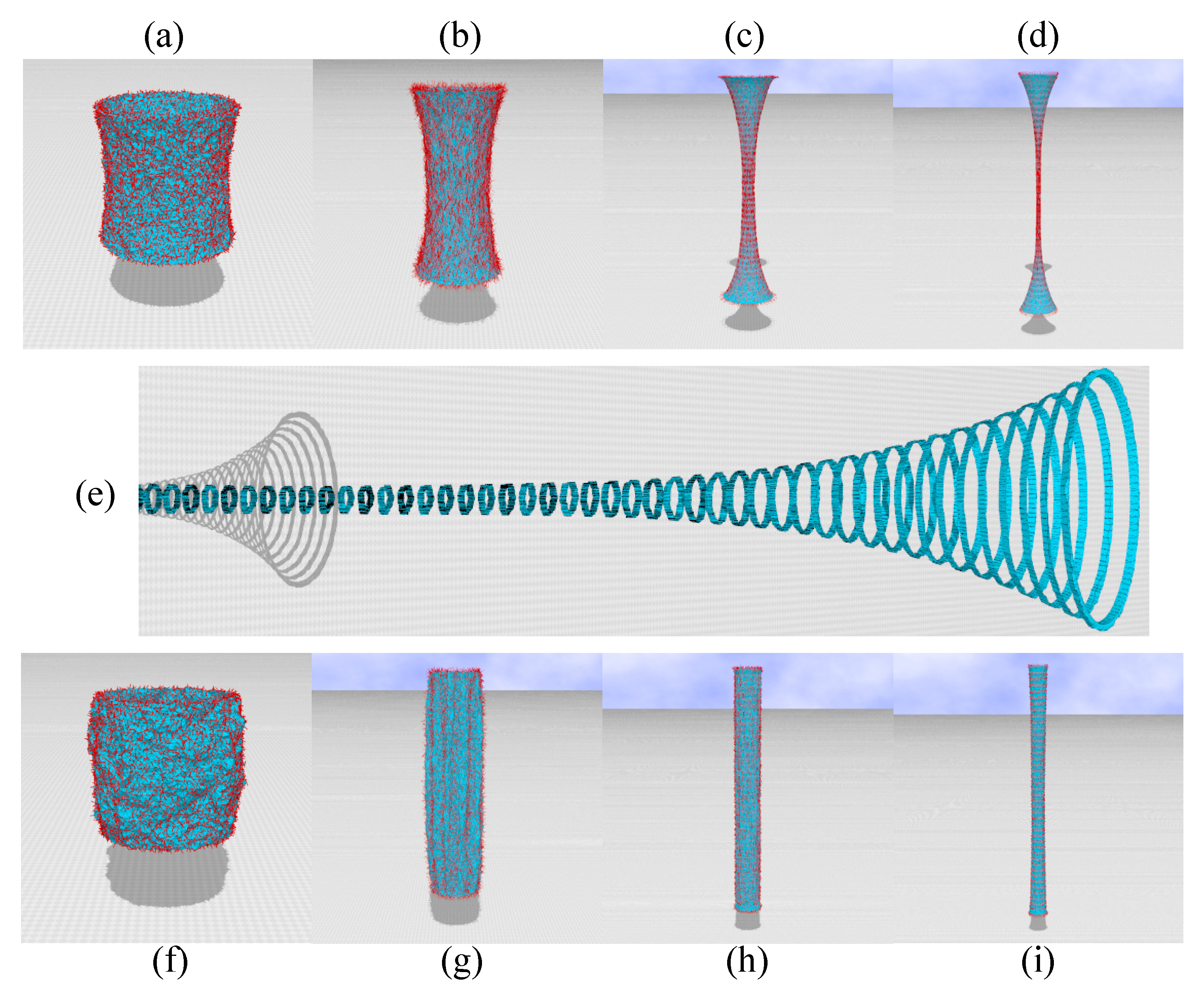
Next, in Figure 11a–e, we show snapshots of 3D cylinders corresponding to the data () in Figure 7a, where the assumed parameters are λ = 0.1 , b = 0.05 , c = 1.5 and κ = 0.5 . The strains ε for these snapshots are given by (a) ε = 0 , (b) ε = 1.16 , (c) ε = 3.36 and (d) ε = 5.40 . The small red lines on the surface of snapshots represent the variable σ . For small and intermediate ε such as in Figure 11a,b, the variable σ is almost random. We can also confirm that, for large ε such as in Figure 11c,d, the variable σ becomes almost parallel to the z direction.
We find from these snapshots in Figure 11a–c that the surfaces maintain the cylindrical shape, though the central part is slightly thin. However, in Figure 11d, which is the case for the largest strain, the central part appears almost string-like. Therefore, to check whether the surface collapses, we show the surface sections in Figure 11e, where almost 2/3 of the surface is shown and rotated by π / 2 from the vertical to the horizontal direction. From Figure 11e, we confirm that the central part of the surface still maintains its surface structure, and, therefore, the free energy formula in Equation (17) pertains; hence, the frame tension formula in Equation (18) can be used with those constricted surfaces.
Figure 11f–i are snapshots corresponding to the data () in Figure 8b, where the assumed parameters are λ = 0 , b = κ = 1 and c = 0.045 . The strains ε for these snapshots are given by (f) ε = 0 , (g) ε = 3.58 , (h) ε = 8 and (i) ε = 12.9 . We find from the snapshots that the surface shape remains almost unchanged even at ε = 12.9 , though the diameter of the central region is slightly thin compared to that of the boundary circle. The reason why the surface in (i) does not shrink similar to that in (d), even though the maximum strain in (i) is almost two times larger than that in (d), is understood from the fact that the combination of the parameters b and c assumed for the data in Figure 7a is different from that for the data in Figure 8a. Indeed, as described in Section 3.1, the combination of the parameters b ( = 0.05 ) c ( = 1.5 ) assumed for τ sim in Figure 7a is different from those ( 1 = ) b c ( = 0.045 ) for τ sim in Figure 8b. This result indicates that the quadratic term S 2 has a nontrivial role in causing such a strong constriction to the surfaces.
Finally, we should like to comment on the other variants of the Finsler geometry model. The role of σ in the Finsler geometry model is assumed to represent the direction of the polymer chains and to have a nonpolar interaction. However, it is also possible to consider σ to be an electric dipole moment or polarization vector p in the polymers and to have polar interactions, as in the Heisenberg spin model for ferromagnetic phase transitions. In this case, σ represents the polarization p , and we have two possibilities for the direction of p —parallel or vertical to the polymer axis. For the parallel case, the Finsler length v i j is defined by Equation (4), while, for the vertical case, it is defined by v i j = | t i j · σ i | + v 0 . We have checked in both cases that the results are relatively close to those presented in this paper and therefore can also be compared to the experimental data.

4. Summary and Conclusions

In this paper, we report the simulation data of the Finsler geometry model for the stress–strain curve of rubbers. The Finsler geometry model for rubber is an extension of the surface model of Helfrich and Polyakov for membranes. We find that several sets of reported experimental data of stress–strain curves up to 1200% can be successfully reproduced by the 3D and 2D Finsler geometry models. Moreover, the results of the 3D Finsler geometry model are consistent with the experimental data as influenced by strain-induced crystallization and the presence of fillers.
We emphasize that the stress τ is calculated without the assumption of affine deformation in the Finsler geometry model. This approach is in sharp contrast to the conventional modeling of the stress–strain curve of rubbers. Indeed, we assume only that the free energy of the macroscopic planar rubber is proportional to τ , which is the macroscopic surface tension. This assumption for τ is physically reasonable because rubbers accumulate elastic energy if their area is increased by an external tensile force. The entropy elasticity, which states that the stress is proportional to the temperature, is also implemented in τ sim .

Author Contributions

H.K. designed the study, performed the modeling and the simulations and wrote the paper. C.B., J.-M.C., G.D., G.S., J.-Y.C., T.T. and L.C. designed and directed the study, evaluated the simulation results and data analyses and critically reviewed the manuscript.

Funding

This work is supported in part by JSPS KAKENHI Grant No. JP17K05149 and the Collaborative Research Project of the Institute of Fluid Science, Tohoku University.

Acknowledgments

The authors acknowledge Eiji Toyoda, Mitsutaka Anzai, and Daisuke Sawahata for the computer simulations and data analyses.

Conflicts of Interest

The authors declare no conflict of interest.

Abbreviations

The following abbreviations are used in this manuscript:
2Dtwo-dimensional
3Dthree-dimensional

Appendix A. Discretization of the Tensile Energy for the 3D Model
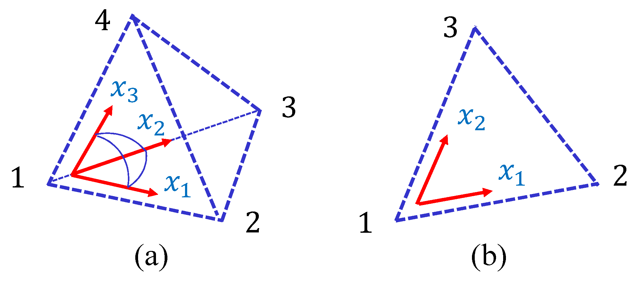
The discretization of these continuous functions on 3D lattices, which are composed of tetrahedrons such as the one in Figure A1a, is straightforward. Though the discrete form of S 1 is exactly the same as that in Ref. [23], we show the discretization technique in this paper in a self-contained way. We assume that a local coordinate origin in a tetrahedron in Figure A1a is at vertex 1, and the corresponding possible coordinate axes x 1 , x 2 , x 3 are fixed as in Figure 4b. Using this local coordinate, we replace the differentials 1 r , 2 r , and 3 r by the differences r 2 r 1 , r 3 r 1 , and r 4 r 1 , respectively. The integral g d 3 x can be replaced by the sum of the tetrahedrons such that tet ( v 12 v 13 v 14 ) 1 . Thus, we have the following discrete Hamiltonians:
S 1 = tet v 12 v 13 v 14 12 2 + v 13 v 12 v 14 13 2 + v 14 v 12 v 13 14 2 , S 2 = tet v 12 3 v 13 v 14 12 4 + v 13 3 v 12 v 14 13 4 + v 14 3 v 12 v 13 14 4 + 2 v 12 v 13 v 14 12 2 13 2 + 2 v 13 v 14 v 12 13 2 14 2 + 2 v 12 v 14 v 13 12 2 14 2 .
It is also possible to assume that the local coordinate origin is at the one of the other three vertices 2, 3, or 4. The corresponding discrete expressions for S 1 and S 2 are simply obtained by replacing the indexes 1 2 , 2 3 , 3 4 , and 4 1 repeatedly. Summing over all possible terms with the factor 1 / 4 and replacing the sum of tetrahedrons tet by the sum of bonds i j with the factor 1 / N ¯ , we have the discrete Hamiltonian
S 1 = i j Γ i j i j 2 , Γ i j = 1 N ¯ tet γ i j ( tet ) , S 2 = i j Γ i j ( 1 ) i j 4 + i j , k l Γ i j , k l ( 2 ) i j 2 k l 2 , Γ i j ( 1 ) = 1 N ¯ tet γ i j ( 1 ) ( tet ) , Γ i j , k l ( 2 ) = 1 N ¯ tet γ i j , k l ( 2 ) ( tet ) .
The symbols γ i j in Γ i j of S 1 in Equation (A2) are given by
γ 12 = 1 4 v 12 v 13 v 14 + v 21 v 23 v 24 , γ 13 = 1 4 v 13 v 12 v 14 + v 31 v 32 v 34 , γ 14 = 1 4 v 14 v 12 v 13 + v 41 v 42 v 43 , γ 23 = 1 4 v 23 v 21 v 24 + v 32 v 31 v 34 , γ 24 = 1 4 v 24 v 21 v 23 + v 42 v 41 v 43 , γ 34 = 1 4 v 34 v 31 v 32 + v 43 v 41 v 42 .
In S 2 , the symbols γ i j ( 1 ) and γ i j , k l ( 2 ) in Γ i j ( 1 ) and Γ i j , k l ( 2 ) are defined by
γ 12 ( 1 ) = 1 6 v 12 3 v 13 v 14 + v 21 3 v 23 v 24 , γ 13 ( 1 ) = 1 6 v 13 3 v 12 v 14 + v 31 3 v 32 v 34 , γ 14 ( 1 ) = 1 6 v 14 3 v 12 v 13 + v 41 3 v 42 v 43 , γ 23 ( 1 ) = 1 6 v 23 3 v 21 v 24 + v 32 3 v 31 v 34 , γ 24 ( 1 ) = 1 6 v 24 3 v 21 v 23 + v 42 3 v 41 v 43 , γ 34 ( 1 ) = 1 6 v 34 3 v 31 v 32 + v 43 3 v 41 v 42 ,
and
γ 12 , 13 ( 2 ) = 1 3 v 12 v 13 v 14 , γ 12 , 14 ( 2 ) = 1 3 v 12 v 14 v 13 , γ 13 , 14 ( 2 ) = 1 3 v 13 v 14 v 12 , γ 21 , 23 ( 2 ) = 1 3 v 21 v 23 v 24 , γ 23 , 24 ( 2 ) = 1 3 v 23 v 24 v 21 , γ 21 , 24 ( 2 ) = 1 3 v 21 v 24 v 23 , γ 31 , 32 ( 2 ) = 1 3 v 31 v 32 v 34 , γ 31 , 34 ( 2 ) = 1 3 v 31 v 34 v 32 , γ 32 , 34 ( 2 ) = 1 3 v 32 v 34 v 31 , γ 41 , 42 ( 2 ) = 1 3 v 41 v 42 v 43 , γ 41 , 43 ( 2 ) = 1 3 v 41 v 43 v 42 , γ 42 , 43 ( 2 ) = 1 3 v 42 v 43 v 41 .
Figure A1. (a) a tetrahedron and a local coordinate origin at vertex 1, where the arrows denote the local coordinate axes; (b) a triangle and a local coordinate origin at vertex 1.
Symmetry 11 01124 g0a1

Appendix B. Discretization of the Tensile and Bending Energies for the 2D Model

The discretization techniques of S 1 and S 2 in the 2D model are exactly the same as those in the 3D model except that triangles instead of tetrahedrons are used for the replacements of the derivations i r ( i = 1 , 2 ) and integration g d 2 x . We have three possible local coordinate origins in a triangle (Figure A1b), and summing over all possible terms with the factor 1 / 3 , we obtain discrete expressions for S 1 , S 2 and S 3 :
S 1 = i j Γ i j i j 2 , Γ i j = 1 N ¯ tet γ i j ( tet ) , S 2 ( σ ) = i j Γ i j ( 1 ) i j 4 + i j , k l Γ i j , k l ( 2 ) i j 2 k l 2 , Γ i j ( 1 ) = 1 N ¯ tet γ i j ( 1 ) ( tet ) , Γ i j , k l ( 2 ) = 1 N ¯ tet γ i j , k l ( 2 ) ( tet ) , S 3 = i j κ i j 1 n i · n j .
For the 2D model, we use the same symbols γ i j , γ i j ( 1 ) and γ i j , k l ( 2 ) for S 1 and S 2 as those in the 3D model; however, no confusion is expected, and these are given by
γ 12 = 1 6 v 12 v 13 + v 21 v 23 , γ 23 = 1 6 v 23 v 21 + v 32 v 31 , γ 31 = 1 6 v 31 v 32 + v 13 v 12 , γ 12 ( 1 ) = 1 6 v 12 3 v 13 + v 21 3 v 23 , γ 23 ( 1 ) = 1 6 v 23 3 v 21 + v 32 3 v 31 , γ 31 ( 1 ) = 1 6 v 31 3 v 32 + v 13 3 v 12 , γ 12 , 13 ( 2 ) = 1 3 v 12 v 13 , γ 21 , 23 ( 2 ) = 1 3 v 21 v 23 , γ 31 , 32 ( 2 ) = 1 3 v 31 v 32 .
We should note that the definition of v i j in the 2D model is exactly the same as that in Equation (4) for the 3D model.
The discretization of the bending energy S 3 is also easy to perform (see Ref. [24], for example). Note that the sum i j in S 3 is performed over the triangles i j , which share the same bond, and n i is defined not at the vertex i but on the triangle i. The symbols κ i j in S 3 are given by
κ 12 = 1 6 v 13 v 12 + v 23 v 21 , κ 23 = 1 6 v 21 v 23 + v 31 v 32 , κ 31 = 1 6 v 32 v 31 + v 12 v 13 .
We should comment on the difference of the coefficients γ i j and Γ i j ( 1 ) , Γ i j , i k ( 2 ) between the 2D and 3D models. First, γ i j in Equation (A7) and κ i j in Equation (A8) of the 2D model are of “degree” 0 with respect to v i j because both of these are rational functions of v i j , and the degree of v i j in the denominator is identical to that in the numerator. In contrast, the coefficients Γ i j ( 1 ) and Γ i j , i k ( 2 ) in Equation (A7) are of degree 2 with respect to v i j as a result of the fact that S 2 in Equation (A6) is not conformally invariant (as mentioned in Section 2.3). In the case of the 3D model, not only S 2 but also S 1 in Equation (A2) is not conformally invariant, and therefore γ i j in Equation (A3) and Γ i j ( 1 ) , Γ i j , i k ( 2 ) in Equations (A4) and (A5) are of degrees 1 and 1, respectively. Both of these degrees in the coefficients of the 3D model are different from those in the 2D model.

References and Notes

  1. Albouy, P.-A. The conformation of poly (dimethylsiloxane) in the crystalline state. Polymer 2000, 41, 3083–3086. [Google Scholar] [CrossRef]
  2. Imbernon, L.; Puachet, R.; Pire, M.; Albouy, P.-A.; Tencé-Giraut, S.; Norves, S. Strain-induced crystallization in sustainably crosslinked epoxidizednatural rubber. Polymer 2016, 93, 189–197. [Google Scholar] [CrossRef]
  3. Candau, N.; Chazeau, L.; Chenal, J.-M.; Gauthier, C.; Ferreira, J.; Munch, E.; Rochas, C. Characteristic time of strain induced crystallization of crosslinked natural rubber. Polymer 2012, 53, 2540–2543. [Google Scholar] [CrossRef] [Green Version]
  4. Toki, S.; Sics, I.; Hsiao, B.S.; Murakami, S.; Tosaka, M.; Poompradub, S.; Kohjiya, S.; Ikeda, Y. Structural developments in synthetic rubbers during uniaxial deformation by in situ synchrotron X-ray diffraction. J. Polym. Sci. B 2004, 42, 956–964. [Google Scholar] [CrossRef]
  5. Treloar, L.R.G. The Physics of Rubber Elasticity, 3rd ed.; Claredon Press: Oxford, UK, 1975. [Google Scholar]
  6. Treloar, L.R.G. Rubber elasticity. Contemp. Phys. 1971, 12, 33–56. [Google Scholar] [CrossRef]
  7. Kuhn, W. Dependence of the average transversal on the longitudinal dimensions of statistical coils formed by chain molecules. J. Polym. Sci. 1946, 1, 380–388. [Google Scholar] [CrossRef]
  8. Kuhn, W. Beziehungen zwischen Molekülgröse, statistischer Molekülgestalt und elastischen Eigenschaften hochpolymerer Stoffe. Kolloid Z. 1936, 76, 258–271. [Google Scholar] [CrossRef]
  9. Flory, P.J. Network topology and the theory of rubber elasticity. Polym. Int. 1985, 17, 96–102. [Google Scholar] [CrossRef]
  10. Tanaka, F. Polymer Physics: Applications to Molecular Association and Thermoreversible Gelation; Cambridge Univ. Press Ithaca: Cambridge, UK, 2011. [Google Scholar]
  11. James, H.M.; Guth, E. Statistical Thermodynamics of Rubber Elasticity. J. Chem. Phys. 1953, 21, 1039–1048. [Google Scholar] [CrossRef]
  12. Wall, F.T. Statistical Thermodynamics of Rubber. III. J. Chem. Phys. 1943, 11, 527–530. [Google Scholar] [CrossRef]
  13. Flory, P.J. Statistical thermodynamics of random networks. Proc. Roy. Soc. Lond. A 1976, 351, 351–380. [Google Scholar] [CrossRef]
  14. Flory, P.J. Principles of Polymer Chemistry; Cornell Univ. Press: Ithaca, NY, USA, 1953. [Google Scholar]
  15. Wall, F.T.; Flory, P.J. Statistical Thermodynamics of Rubber Elasticity. J. Chem. Phys. 1951, 19, 1435–1439. [Google Scholar] [CrossRef]
  16. Flory, P.J. Statistical Mechanics of Swelling of Network Structures. J. Chem. Phys. 1950, 18, 108–111. [Google Scholar] [CrossRef]
  17. Mooney, M. A Theory of Large Elastic Deformation. J. Appl. Phys. 1940, 11, 582–592. [Google Scholar] [CrossRef]
  18. Rivlin, R.S. Large elastic deformations of isotropic materials I. Fundamental concepts. Phil. Trans. R. Soc. Lond. Soc. A 1948, 240, 459–490. [Google Scholar] [CrossRef]
  19. Rivlin, R.S. Large elastic deformations of isotropic materials IV. Further depelopements of the general theory. Phil. Trans. R. Soc. Lond. Soc. A 1948, 241, 379–397. [Google Scholar] [CrossRef]
  20. Deam, R.T.; Edwards, F.R.S. The theory of rubber elasticity. Phil. Trans. Roy. Soc. Lond. 1976, 280, 317–353. [Google Scholar] [CrossRef]
  21. Urayama, K. An experimentalist’s view of the physics of rubber elasticity. J. Polym. Sci. B 2006, 44, 3440–3444. [Google Scholar] [CrossRef]
  22. Koibuchi, H.; Sekino, H. Monte Carlo studies of a Finsler geometric surface model. Phys. A 2014, 393, 37–50. [Google Scholar] [CrossRef] [Green Version]
  23. Osari, K.; Koibuchi, H. Finsler geometry modeling and Monte Carlo study of 3D liquid crystal elastomer. Polymer 2017, 114, 355–369. [Google Scholar] [CrossRef]
  24. Takano, Y.; Koibuchi, H. J-shaped stress–strain diagram of collagen fibers: Frame tension of triangulated surfaces with fixed boundaries. Phys. Rev. E 2017, 95, 042411. [Google Scholar] [CrossRef]
  25. Mitsuhashi, K.; Ghosh, S.; Koibuchi, H. Mathematical modeling and simulations for large-strain J-shaped diagrams of soft biological tissues. Polymers 2018, 10, 715. [Google Scholar] [CrossRef] [PubMed]
  26. Koibuchi, H.; Bernard, C.; Chenal, J.M.; Diguet, G.; Sebald, G.; Cavaille, J.Y.; Takagi, T.; Chazeau, L. Mathematical Modeling of Rubber Elasticity. J. Phys. Conf. Ser. 2018, 1142, 012081. [Google Scholar] [CrossRef]
  27. Lebwohl, P.A.; Lasher, G. Nematic-Liquid-Crystal Order?A Monte Carlo Calculation. Phys. Rev. A 1972, 6, 426–429. [Google Scholar] [CrossRef]
  28. Wheater, J.F. Random surfaces: From polymer membranes to strings. J. Phys. A Math. Gen. 1994, 27, 3323–3354. [Google Scholar] [CrossRef]
  29. Fournier, J.-B.; Barbetta, C. Direct Calculation from the Stress Tensor of the Lateral Surface Tension of Fluctuating Fluid Membranes. Phys. Rev. Lett. 2008, 100, 078103. [Google Scholar] [CrossRef] [PubMed]
  30. Foty, R.A.; Forgacs, G.; Pfleger, C.M.; Steinberg, M.S. Liquid properties of embryonic tissues: Measurement of interfacial tensions. Phys. Rev. Lett. 1994, 72, 2298–2301. [Google Scholar] [CrossRef] [PubMed]
  31. Creutz, M. Quarks, Gluons and Lattices; Cambridge University Press: Cambridge, UK, 1983. [Google Scholar]
  32. Schoeberl, J. Netgen Mesh Generator, a Free Software for 3D Meshing. Available online: https://ngsolve.org/ (accessed on 1 January 2016).
  33. Chern, S.-S. Finsler Geometry Is Just Riemannian Geometry without the Quadratic Restriction. In Notices of the AMS; American Mathematical Society: Providence, RI, USA, 1996; pp. 959–963. [Google Scholar]
  34. Matsumoto, M. Foundations of Finsler Geometry and Special Finsler Spaces; Kaiseisya: Tokyo, Japan, 1986. [Google Scholar]
  35. Matsumoto, M. Keiryou Bibun Kikagaku; Shokabo: Tokyo, Japan, 1975. (In Japanese) [Google Scholar]
  36. Bao, D.; Chern, S.-S.; Shen, Z. An Introduction to Riemann-Finsler Geometry, GTM 200; Springer: New York, NY, USA, 2000. [Google Scholar]
  37. The variable σ represents the “mean value” of the direction of the polymer chains at a given point in the material, and this mean direction is identical to that expressed by σ . For this reason, the directions are represented by the left-right arrows in Figure 4c.
  38. Helfrich, W. Elastic Properties of Lipid Bilayers: Theory and Possible Experiments. Z. Naturforsch C 1973, 28, 693–703. [Google Scholar] [CrossRef]
  39. Polyakov, A.M. Fine structure of strings. Nucl. Phys. B 1986, 268, 406–412. [Google Scholar] [CrossRef]
  40. Kantor, Y.; Karder, M.; Nelson, D.R. Tethered surfaces: Statics and dynamics. Phys. Rev. A 1987, 35, 3056–3071. [Google Scholar] [CrossRef] [PubMed]
  41. Kantor, Y.; Nelson, D.R. Phase Transitions in Flexible Polymeric Surfaces. Phys. Rev. A 1987, 36, 4020–4032. [Google Scholar] [CrossRef] [PubMed]
  42. Bowick, M.; Travesset, A. The statistical mechanics of membranes. Phys. Rep. 2001, 344, 255–308. [Google Scholar] [CrossRef] [Green Version]
  43. Wiese, K.J. Polymerized Membranes, a Review. In Phase Transitions and Critical Phenomena 19; Domb, C., Lebowitz, J.L., Eds.; Academic Press: London, UK, 2000; pp. 253–498. [Google Scholar]
  44. Nelson, D. The Statistical Mechanics of Membranes and Interfaces. In Statistical Mechanics of Membranes and Surfaces, 2nd ed.; Nelson, D., Piran, T., Weinberg, S., Eds.; World Scientific: Singapore, 2004; pp. 1–17. [Google Scholar]
  45. Gompper, G.; Kroll, D.M. Triangulated-surface Models of Fluctuating Membranes. In Statistical Mechanics of Membranes and Surfaces, 2nd ed.; Nelson, D., Piran, T., Weinberg, S., Eds.; World Scientific: Singapore, 2004; pp. 359–426. [Google Scholar]
  46. Doi, M.; Edwards, S.F. The Theory of Polymer Dynamics; Oxford University Press: Oxford, UK, 1986. [Google Scholar]
  47. David, F. Geometry and Field Theory of Random Surfaces and Membranes. In Statistical Mechanics of Membranes and Surfaces, 2nd ed.; Nelson, D., Piran, T., Weinberg, S., Eds.; World Scientific: Singapore, 2004; pp. 149–209. [Google Scholar]
  48. Stress is normally expressed by the symbol σ, however, this symbol σ is already used for the directional degree of freedom of polymers. For this reason, the symbol τ is used instead of σ for stress in this paper.
  49. Metropolis, N.; Rosenbluth, A.W.; Rosenbluth, M.N.; Teller, A.H. Equation of State Calculations by Fast Computing Machines. J. Chem. Phys. 1953, 21, 1087–1092. [Google Scholar] [CrossRef] [Green Version]
  50. Landau, D.P. Finite-size behavior of the Ising square lattice. Phys. Rev. B 1976, 13, 2997–3011. [Google Scholar] [CrossRef]
  51. Pradhan, S.; Costa, F.R.; Wagenknecht, U.; Jehnichen, D.; Bhowmick, A.K.; Heinrich, G. Elastomer/LDH nanocomposites: Synthesis and studies on nanoparticle dispersion, mechanical properties and interfacial adhesion. Eur. Polym. J. 2008, 44, 3122–3132. [Google Scholar] [CrossRef]
  52. The high-precision number assumed for c does not always imply that the results are very sensitive to c. In the simulation program, the parameter c′(=(2/3)c) was used instead of c. As a result, the simple input numbers c′ = 0.7 and c′ = 0.03 turn to be c = 1.05 and c = 0.045, respectively.
  53. Shahedifar, V.; Rezadoust, A.M. Thermal and mechanical behavior of cotton/vinyl ester composites: Effects of some flame retardants and fiber treatment. J. Reinf. Plast. Compos. 2013, 32, 681–688. [Google Scholar] [CrossRef]
  54. Kawano, Y.; Wang, Y.; Palmer, R.A.; Aubuchon, S.R. Stress-Strain Curves of Nafion Membranes in Acid and Salt Forms. Polim. Cienc. Tecnol. 2002, 12, 96–101. [Google Scholar] [CrossRef] [Green Version]
  55. In the hysteresis simulation for the variation of the strain ϵ, the final configuration of the previous simulation is used as an input of the following simulation, where the total number of Monte Carlo sweep is always kept small so that the configuration may not be convergent.
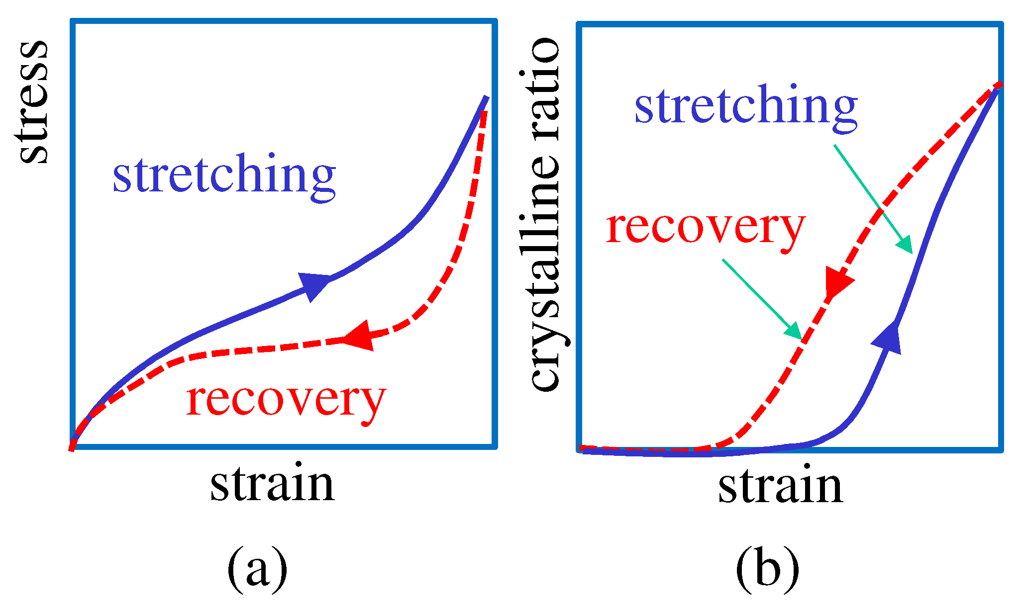
Figure 1. (a) scheme of the stress–strain curves usually obtained with a natural rubber from its tensile loading and unloading; (b) scheme of the concomitant evolution of the strain-induced crystallization.
Symmetry 11 01124 g001
Figure 2. (a) illustrations of affine deformation in a continuum material, in which the microscopic strains / are exactly the same as the macroscopic strain L / L ; (b) illustrations of the microscopic internal structure of rubbers without strain (upper) and with strain (lower). In the dashed circle (upper), the polymer directions are almost random or isotropic, while in the dashed ellipse (lower), the polymers align along the strain direction and partly crystallize (strain-induced crystallization). The ”polymer directions” are used in a coarse-grained manner representing the directions of the polymer segments.
Symmetry 11 01124 g002
Figure 3. (a) a thick cylinder discretized by tetrahedrons for the 3D model; (b) a cylindrical surface discretized by triangles for the 2D model; (c) illustration for the construction of a cylindrical surface from a rectangular surface by removing a pair of boundaries. The cylinder is stretched in the height (or H) direction, whereas the surfaces in Figure 2a,b are stretched in the horizontal direction.
Symmetry 11 01124 g003
Figure 4. (a) a part of the 3D material with the position vector r in R 3 ; (b) a tetrahedron of vertices 1, 2, 3 and 4, where the three thin arrows denote the local coordinate axes, and (c) directions of the polymer represented by the variables ± σ . The term ± σ represents a mean value of directions of several polymer segments at the vertex (or crosslinker) position. The material, a part of which is shown in (a), is discretized by tetrahedrons in (b) to define the discrete Hamiltonian, and these tetrahedrons form a 3D thick cylinder in Figure 3b. The dashed line connecting two vertices in (c) corresponds to an edge of a tetrahedron in (b). The Finsler length v 12 in Equation (4) along the edge 12 is defined by using the variable σ 1 and the unit tangential vector t 12 in (b).
Symmetry 11 01124 g004
Figure 5. (a) an illustration of the 2D cylindrical surface of fixed height H and diameter D 0 of the boundaries, where the vertices are allowed to fluctuate along the boundary circles; (b) the boundary vertices are also allowed to fluctuate into the height direction within the distance ± δ B from the position fixed by H.
Symmetry 11 01124 g005
Figure 6. (a) a part of the smooth 2D cylindrical surface in R 3 ; this smooth surface is discretized by triangles; (b) a tangential plane at the vertex i, which is defined by the unit normal vector N i . The parallel component σ i of σ i is used to define the energy S 0 of the 2D model.
Symmetry 11 01124 g006
Figure 7. The simulation results of the stress–strain curves by the Finsler geometry model and the corresponding simulated order parameters M are plotted in (ad). The plotted data with the symbol (×) in (a,c) are the experimental data τ exp of EL10 in Ref. [51]. The parameter λ is varied in (a,b), while in (c,d), κ is varied. The symbol τ on the vertical axes in (a,c) represents τ exp or τ sim .
Symmetry 11 01124 g007
Figure 8. The simulation results of the stress–strain curves and order parameter M by the Finsler geometry model are plotted in (ad), and the plotted data with the symbol (×) are the experimental data τ exp of (a) XL10 and (c) XL5 in Ref. [51]. The parameter c is varied in both (a,b) and (c,d).
Symmetry 11 01124 g008
Figure 9. 2D model simulation results of the stress–strain data τ exp and order parameters M are plotted in (a), (b) and (c), (d). The experimental data τ exp in Ref. [53] are plotted in (a) and (c) with the symbol (×). The parameter λ varies in (a), (b), and κ varies in (c), (d).
Symmetry 11 01124 g009
Figure 10. (a) the parameters τ sim vs. ε obtained with b = 1 , c = 1.5 , κ = 4 and two different λ of λ = 0 and λ = 2 ; (b) the corresponding M vs. ε ; (c) τ sim vs. ε obtained with λ = 0 , b = 1 , κ = 4 and two different c of c = 0.3 and c = 1.5 ; (d) the corresponding M vs. ε .
Symmetry 11 01124 g010
Figure 11. The snapshots of cylindrical surfaces corresponding to the data () in Figure 7a with strains (a) ε = 0 ; (b) ε = 1.16 ; (c) ε = 3.36 ; (d) ε = 5.40 ; and (e) the rotated surface sections of a part (more than half) of the snapshot in (d). The snapshot in (e) is rotated by π / 2 . The snapshots in (fi) correspond to the data () in Figure 8b with strains (f) ε = 0 , (g) ε = 3.58 , (h) ε = 8 , and (i) ε = 12.9 . The small red lines represent the variable σ .
Symmetry 11 01124 g011
Table 1. The lattice spacing a assumed to obtain τ sim (in Equation (20)) plotted in Figure 7, Figure 8 and Figure 9.
FigureModelData ()Data ()Data ()
Figure 7a3D 9.434 × 10 10 1.034 × 10 9 1.109 × 10 9
Figure 7c3D 9.366 × 10 10 9.819 × 10 10 8.952 × 10 10
Figure 8a3D 1.029 × 10 9 9.094 × 10 10 1.024 × 10 9
Figure 8c3D 8.562 × 10 10 9.240 × 10 10 8.149 × 10 10
Figure 9a2D 5.675 × 10 9 6.132 × 10 9 5.152 × 10 9
Figure 9c2D 5.187 × 10 9 5.390 × 10 9 4.963 × 10 9