Research on an Electromagnetic Interference Test Method Based on Fast Fourier Transform and Dot Frequency Scanning for New Energy Vehicles under Dynamic Conditions

Abstract

In recent years, electromagnetic interference (EMI) of new energy vehicles, including difference mode symmetric interference and common mode asymmetry interference, has attracted the attention of many scholars. So far, EMI tests for new energy vehicles under steady conditions cannot reflect the actual EMI of the running vehicle. The results of EMI test methods based on fast Fourier transform (FFT) under dynamic conditions have worse frequency resolutions, and frequency/amplitude accuracy has low precision. Therefore, this paper proposes an EMI test method based on FFT and dot frequency scanning (DFS) for new energy vehicles under dynamic conditions. The identification method for accelerating, sliding, and braking conditions is studied. A comprehensive EMI key evaluation index system for new energy vehicles is built, including characteristic points with maximum amplitude, area, ratio, and density coefficients for high-amplitude characteristic points. Among them, the maximum amplitude is an index to evaluate extreme values. The ratio of high-amplitude characteristic points is a comprehensive index to evaluate the overall region. The density coefficient is an index to evaluate the local region. Finally, this method is applied to three vehicles. With the same instruments, by reducing the FFT frequency span, the frequency resolution and frequency accuracy increase. The results indicate that the EMI of new energy vehicles can be tested under dynamic conditions with high accuracy according to the operable evaluation indexes.

1. Introduction

Nowadays, new energy vehicles are rapidly developed and have become an important means of transportation [1,2]. However, compared to other types of vehicles, new energy vehicles have more electronic components, which are also more complex. In charging and discharging states, serious electromagnetic interference (EMI) occurs, including difference mode symmetric interference and common mode asymmetry interference [3]. EMI testing is one of the most important tests for new energy vehicles. The current EMI test standards for new energy vehicles (e.g., CISPR 12:2009 [4], ECE 10.05 [5], SAE J551-5-2012 [6], GB/T 18387-2017 [7], etc.) only stipulate that the vehicle is tested under steady conditions [8] (e.g., SAE J551-5-2012: when under BRAKE APPLIED, CREEP, and CRUISE steady conditions, the vehicle conditions are constant). Under steady conditions, the EMI test cannot truly reflect the EMI of the running vehicle. SAE J551-5-2012 noticed this problem and indicated that the EMI test standard for dynamic conditions (where the driving conditions change) is still under study [9,10,11]. Therefore, it is very urgent to study EMI testing technology for new energy vehicles under dynamic conditions.

The EMI peak test for vehicles under steady conditions usually uses frequency sweeping. SAE J551-5-2012 specifies a minimum dwell time of 10 ms for a single frequency. It takes tens of seconds to complete a spectrogram, and the amplitude accuracy is ±0.36 dB, which cannot satisfy dynamic conditions. The previous study [12] used dot frequency scanning (DFS) to study the relationship between engine conditions and EMI at a single frequency. EMI testing under dynamic conditions in the full frequency range was not able to be covered. Another study [13] used frequency sweeping to study conducted interference in start-up mode, idling mode, electric mode, and charging mode of a hybrid electric vehicle. But it did not study the changing EMI in the time domain with these conditions. Authors in [14] showed spectrograms measured in the vehicle with the vertical time axis under different driving conditions (low and high speed, acceleration, and deceleration). However, it did not show the speed/acceleration curves that matched the spectrograms. Considering that a fast Fourier transform (FFT) spectrum analysis can capture transient interference, it only takes 24 ms to complete a spectrogram at the same time. Therefore, FFT spectrum analyses are more in line with the requirements of EMI testing under dynamic conditions. The literature [15] developed an EMI test method based on FFT for new energy vehicles under dynamic conditions. The EMI test subsystem and the roller subsystem worked together under computer control to form an integrated measurement system. The amplitude accuracy was ±1.31 dB, which is far larger than ±0. 36 dB of frequency sweeping. Based on the FFT spectrum analysis results of the literature [15], this paper proposes a method to determine the characteristic points to carry out a precise sweep, consisting of both FFT spectrum analysis and DFS (the amplitude accuracy was also ±0.36 dB). Speed and EMI of a narrower frequency span with the time axis under different driving conditions can also be measured.

The remainder of this paper is structured as follows. In Section 2, the framework of the EMI test, based on FFT and DFS for new energy vehicles under dynamic conditions, is introduced and analyzed. The problem that needs to be solved is put forward. In Section 3, the dynamic conditions of accelerating, sliding, and braking conditions are studied, and an identification method is proposed after the speed and acceleration features of the dynamic conditions are analyzed. In Section 4, research on the method to determine characteristic points is carried out. EMI evaluation indexes for new energy vehicles under dynamic condition are proposed to determine the characteristic points. In Section 5, the implementation, experimental research, and analysis of results are explained. Implementation of the EMI test and experimental system are introduced, showing that the proposed EMI test method, based on FFT and DFS for new energy vehicles under dynamic conditions, is correct and effective. In Section 6, conclusions are provided, and the direction of future work is elaborated.

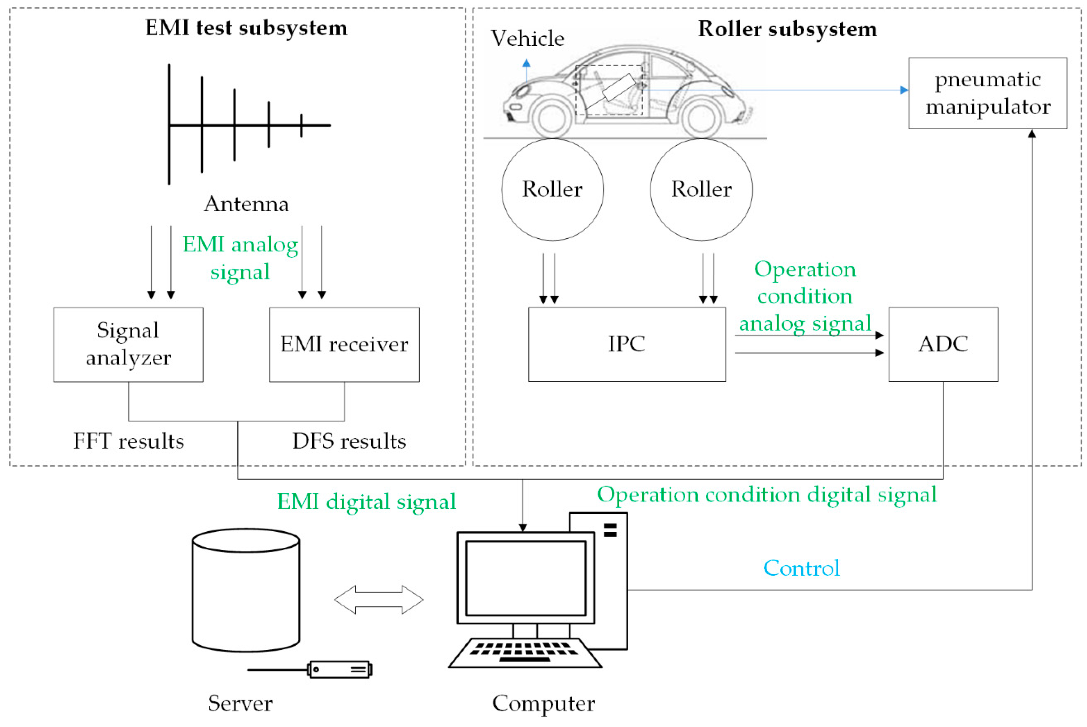
2. Framework of the Electromagnetic Interference (EMI) Test Based on Fast Fourier Transform (FFT) and Dot Frequency Scanning (DFS) for New Energy Vehicles under Dynamic Conditions

The framework of EMI testing, based on FFT and DFS for new energy vehicles under dynamic conditions, is illustrated in Figure 1, which comprises an EMI test subsystem, a roller subsystem, and a computer. The EMI test subsystem and roller subsystem work together under computer control, forming an integrated measurement system. The EMI test subsystem includes an antenna, a signal analyzer, and an EMI receiver. After receiving the radio-frequency (RF) signal, the cable transmits analog voltage to the signal analyzer and EMI receiver. Then, the signal analyzer and EMI receiver send the EMI data to the computer through a network port. The roller subsystem includes a chassis dynamometer, an industrial personal computer (IPC), an analog to digital converter (ADC), and a pneumatic manipulator. The chassis dynamometer contains a variety of sensors to acquire speed, torque, and other physical quantities, whose analog voltages are transmitted to the IPC, then output to the ADC by bayonet nut connectors (BNCs). The ADC connects the IPC and computer to convert the analog signal into a digital signal, and the computer obtains the condition parameters, such as real-time speed of the vehicle, through the ADC. A pneumatic manipulator is placed in the driving position of the vehicle, and two pneumatic arms, respectively, press on the accelerator pedal and brake pedal. The vehicle is controlled by the computer according to speed and acceleration feedback. Through the LabVIEW driver provided by the signal analyzer, EMI receiver, ADC, and pneumatic manipulator, the computer uses LabVIEW to integrate them all with the ethernet port to form an integrated EMI test system based on FFT and DFS for new energy vehicles under dynamic conditions.

Figure 2 is the schematic of the EMI test based on FFT and DFS for new energy vehicles under dynamic conditions. Figure 2a shows an analysis of the rough sweep with the FFT spectrum, and Figure 2b shows the precise sweep process with FFT and DFS. The test includes the rough sweep and precise sweep. The rough sweep analyzes various dynamic conditions of vehicle, including accelerating, sliding, and braking conditions, which can be seen in the upper part of Figure 2a. The abscissa is time, and the ordinate is speed. An analysis of the FFT spectrum of the magnetic field’s radiation emission intensity is carried out to obtain the EMI intensity graph, which can be seen in the lower part of Figure 2a. The abscissa is time, and the ordinate is frequency. Different colors are used to distinguish the amplitude. The precise sweep also completes the same dynamic conditions of the vehicle as the rough sweep, which can be seen in the upper part of Figure 2b. The abscissa is time, and the ordinate is speed. Results of the DFS magnetic field’s radiation emission is carried out to obtain the EMI amplitude graph, which can be seen in the lower part of Figure 2b. The abscissa is time, and the ordinate is amplitude.

The rough sweep and precise sweep are two separate processes. Only when the driving conditions of rough sweep and precise sweep are completely consistent will the precise process be meaningful. In the current study, the pneumatic manipulator is controlled only by the air pressure. Control precision is not enough. Driving conditions during rough sweep and precise sweep are difficult to equally maintain. However, condition parameters such as speed and acceleration during the precise sweep process can be used to identify various conditions. This can make sure the precise sweep conditions correspond to those of the rough sweep. Then, DFS is performed on the corresponding conditions. At the same time, speed and acceleration constantly change when the vehicle accelerates, slides, and brakes. Every frame of the FFT spectrum corresponds to different speeds and accelerations. The EMI is much more complicated than the steady conditions. The point with the maximum subtraction value between the measured value and relevant standard limit in a single spectrogram is called the characteristic point. Ideally, each characteristic point needs DFS. In fact, both identification conditions and changing sweep frequency on the EMI receiver take some time. It is difficult to perform DFS on every characteristic point under dynamic conditions. Choosing the characteristic points for further sweeping from so many points is important. Therefore, in order to achieve an EMI test based on FFT and DFS for new energy vehicles under dynamic conditions, it is necessary to study the methods to identify dynamic conditions and determine characteristic points.

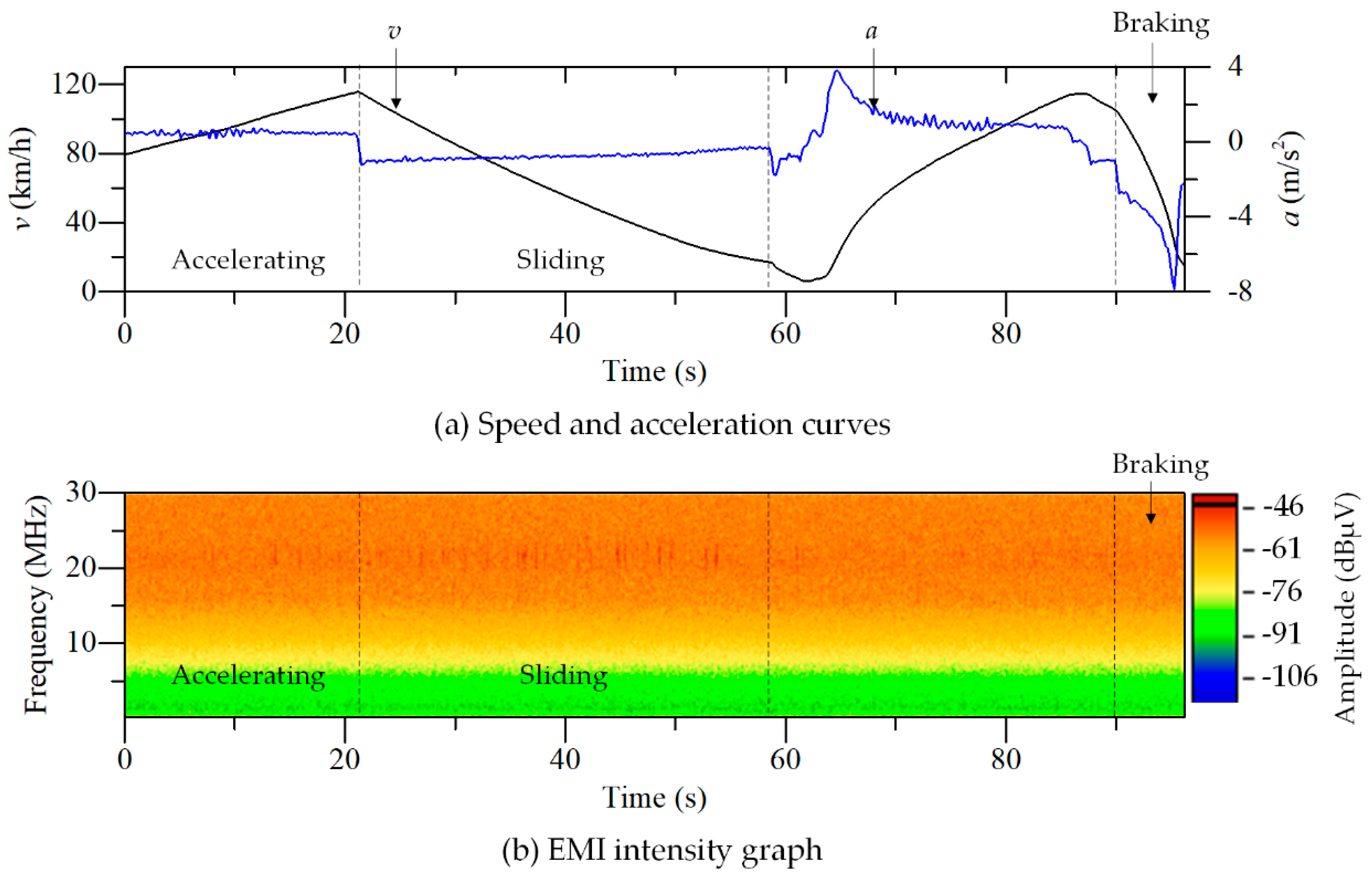
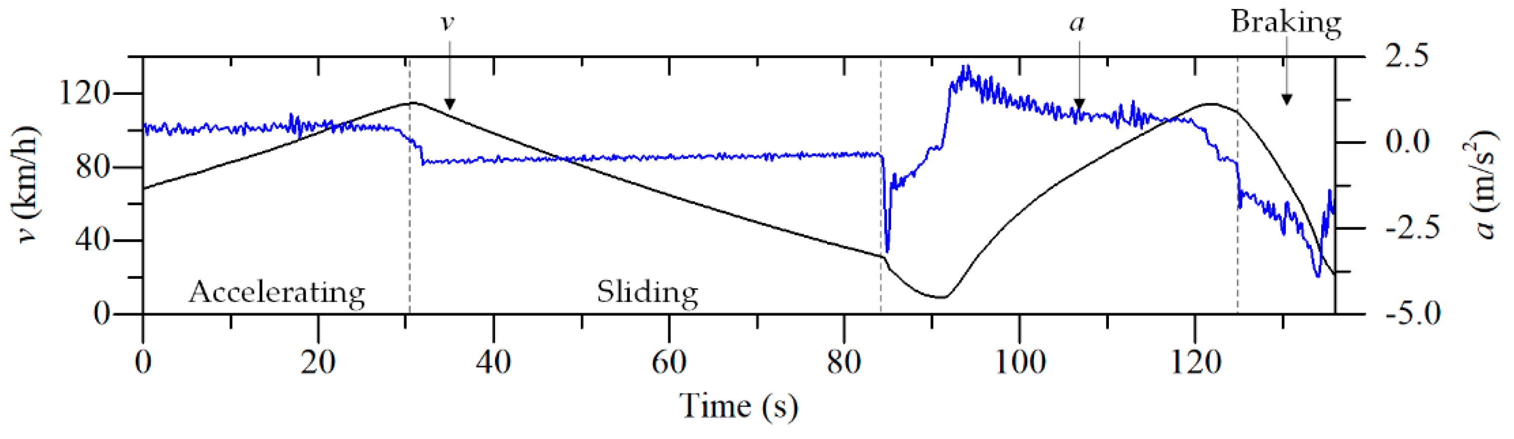
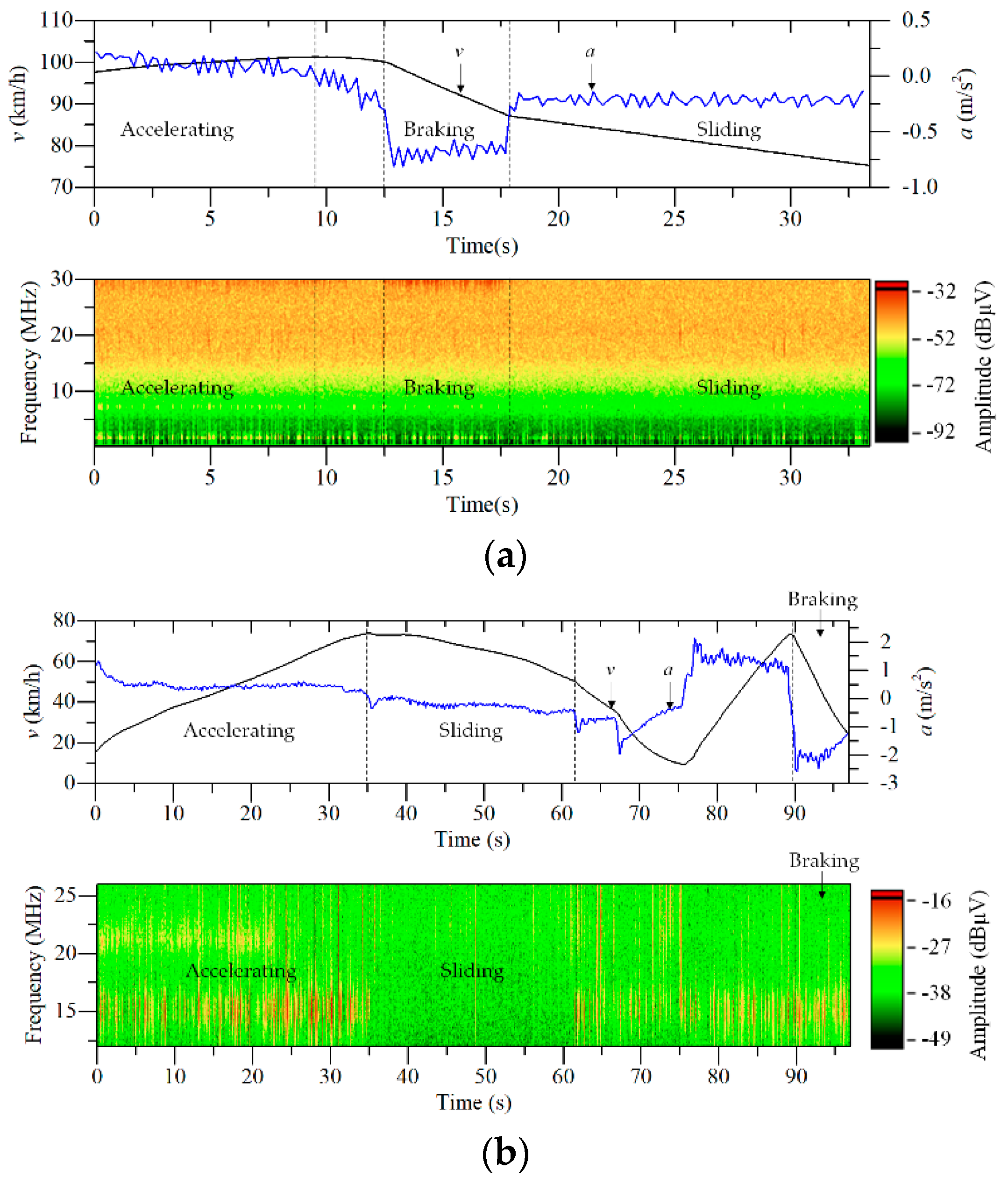
3. Identification Method for Accelerating, Sliding, and Braking Conditions

The method to identify accelerating, sliding, and braking conditions is mainly based on different features of different dynamic conditions. Suppose there are n measured values of speed in a very short time, t_observe. Then, we have the measured values of speed, $V_{\mathrm{measured}}=\left[v_1,v_2,\dots ,v_i,\dots ,v_n\right]$, and the calculated values of acceleration, $A_{\mathrm{calculated}}=$$\left[a_1,a_2,\dots ,a_i,\dots \right]$. The minimum speed in $t_{\mathrm{observe}}$ is $v_{\min }$, $v_{\min }=\min \left\{V_{\mathrm{measured}}\right\}$. The minimum acceleration is $a_{\min }$, $a_{\min }=\min \left\{A_{\mathrm{calculated}}\right\}$. The maximum acceleration is $a_{\max }$, $a_{\max }=\max \left\{A_{\mathrm{calculated}}\right\}$. Features of different dynamic conditions of new energy vehicles are shown in

Table 1. Features of different dynamic condition of new energy vehicles.

	Acceleration	Sliding	Braking
Features of speed and acceleration	$a_i\ge a_{\min }>a_{\mathrm{T}\_\mathrm{acc}}>0$	$v_{\mathrm{idling}}<v_{\min }\le v_i$, $a_{\max }<-a_{\mathrm{T}\_\mathrm{slide}}$	$a_i\le a_{\max }<a_{\mathrm{slide}}-a_{\mathrm{T}\_\mathrm{brake}}<0$

. The physical significance is as follows:

(1)

When the new energy vehicle is accelerating, $a_i>0$, and then $a_{\min }>0$. To avoid misjudgments, a small, positive threshold, $a_{\mathrm{T}\_\mathrm{acc}}$, is introduced. Therefore, $a_i\ge a_{\min }>a_{\mathrm{T}\_\mathrm{acc}}>0$. On the other hand, if the situation when $a_{\min }>a_{\mathrm{T}\_\mathrm{acc}}$ is detected, it indicates that the new energy vehicle is accelerating.

(2)

When the new energy vehicle is sliding, $v_{\mathrm{idling}}<v_i$ and $a_i<0$, then $v_{\mathrm{idling}}<v_{\min }\le v_i$ and $a_{\max }<0$. To avoid misjudgments, a small, negative threshold, $-a_{\mathrm{T}\_\mathrm{slide}}$, is introduced. Therefore, $v_{\mathrm{idling}}<v_{\min }\le v_i$ and $a_{\max }<-a_{\mathrm{T}\_\mathrm{slide}}$. On the other hand, if the situation when $v_i\ge v_{\min }>v_{\mathrm{idling}}$ and $a_{\max }<-a_{\mathrm{T}\_\mathrm{slide}}$ is detected, it indicates that the new energy vehicle is sliding.

(3)

When the new energy vehicle is braking, $a_i<a_{\mathrm{slide}}<0$, then $a_i\le a_{\max }<a_{\mathrm{slide}}<0$. To avoid misjudgments, a small, negative threshold, $-a_{\mathrm{T}\_\mathrm{brake}}$, is introduced. Therefore, $a_i\le a_{\max }<a_{\mathrm{slide}}-a_{\mathrm{T}\_\mathrm{brake}}<0$. On the other hand, if the situation when $a_i\le a_{\max }<a_{\mathrm{slide}}-a_{\mathrm{T}\_\mathrm{brake}}$ is detected, it indicates that the new energy vehicle is braking.

Figure 3 shows the identification of results from dynamic conditions. The abscissa is time (s). The ordinate is speed (km/h) and acceleration (m/s²). According to the features of speed and acceleration, the dynamic conditions of the vehicle during the period from 0 to 43.5 s can be identified, which consist of 0~5.6 s (accelerating), 5.6~8.0 s (sliding), 8.0~9.2 s (braking), 9.2~12.3 s (sliding), 12.3~20.8 s (accelerating), 20.8~25.3 s (sliding), 25.3~27.0 s (braking), 27.3~30.5 s (sliding), 30.5~40.2 s (accelerating), and 40.2~43.5 s (sliding). Based on the features of speed and acceleration, different dynamic conditions can be identified from any group of speed and acceleration curves. In steady conditions, there is no dynamic accelerating, sliding, and braking conditions but only idling, cruising, and steady braking conditions. EMI is more in line with actual driving conditions under dynamic conditions for changing speed.

4. Method to Determine Characteristic Points

Under steady conditions, $v=\mathrm{const}$ and $a=0$. According to a spectrogram of the frequency sweep with lower sweeping speed, a characteristic point corresponding to the maximum amplitude can be obtained. As multiple spectrograms with faster speeds were obtained from FFT spectrum analyses, each spectrogram is a repeated test. Every spectrogram has a characteristic point. Among all characteristic points, the characteristic point corresponding to the maximum amplitude is the final characteristic point.

A schematic of EMI test results based on FFT for new energy vehicles under dynamic conditions is shown in Figure 4. The upper graph shows the speed and acceleration curves, whose x coordinate is time and y coordinate is speed/acceleration. The lower graph shows the 3D diagram of the FFT spectrum analysis, whose x coordinate is time, y coordinate is amplitude, and z coordinate is frequency. It can be seen that the speed and acceleration under dynamic conditions change all the time. The speeds/accelerations of multiple spectrograms from FFT spectrum analyses, as well as the characteristic points, are different, which should be paid attention to under dynamic conditions. Therefore, the method to determine characteristic points under dynamic conditions is more complicated than the method under steady conditions with constant speed. Moreover, in applying FFT spectrum analyses to EMI, the frequency resolution accuracy is low, and the exact characteristic points under dynamic conditions need further research.

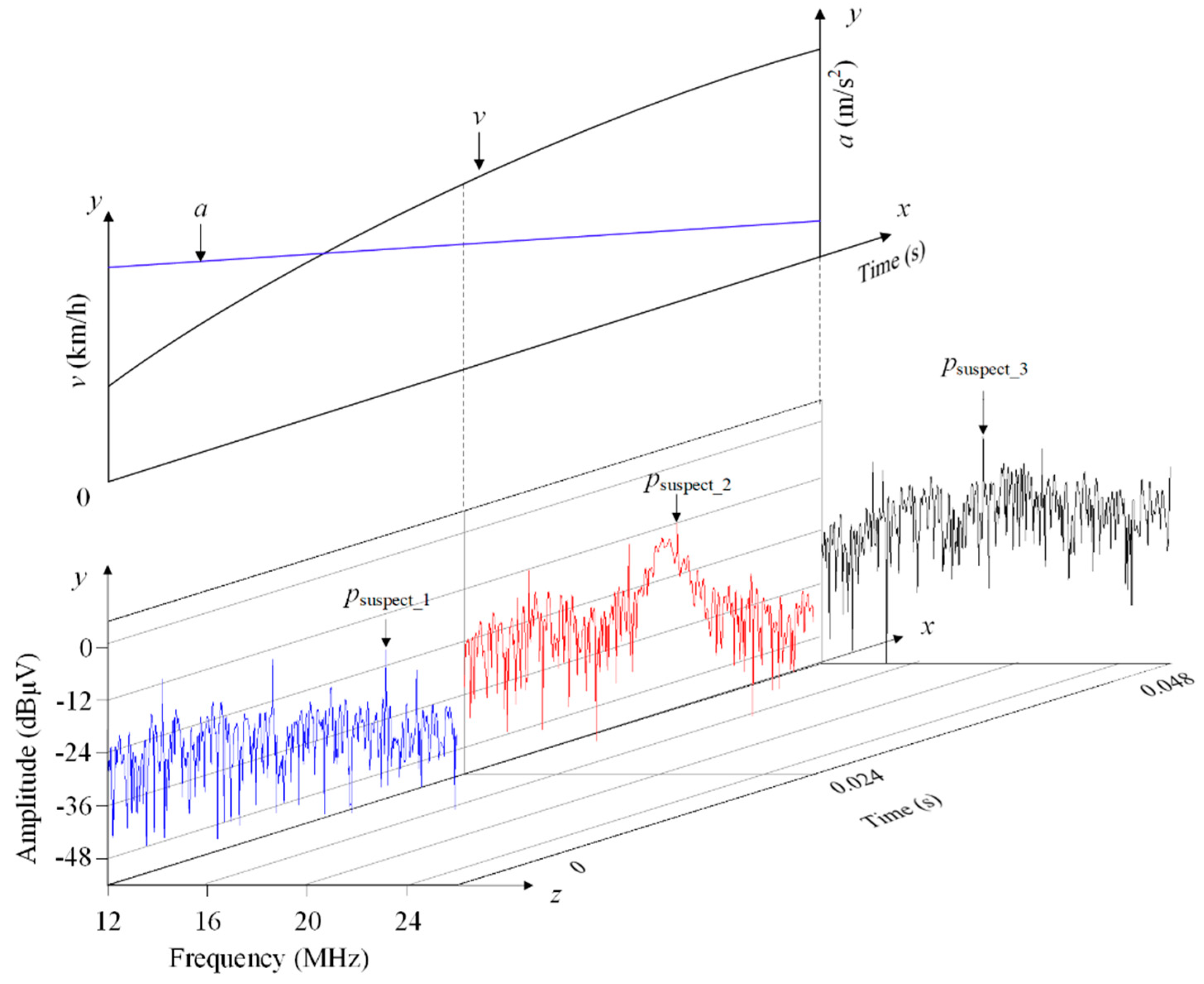
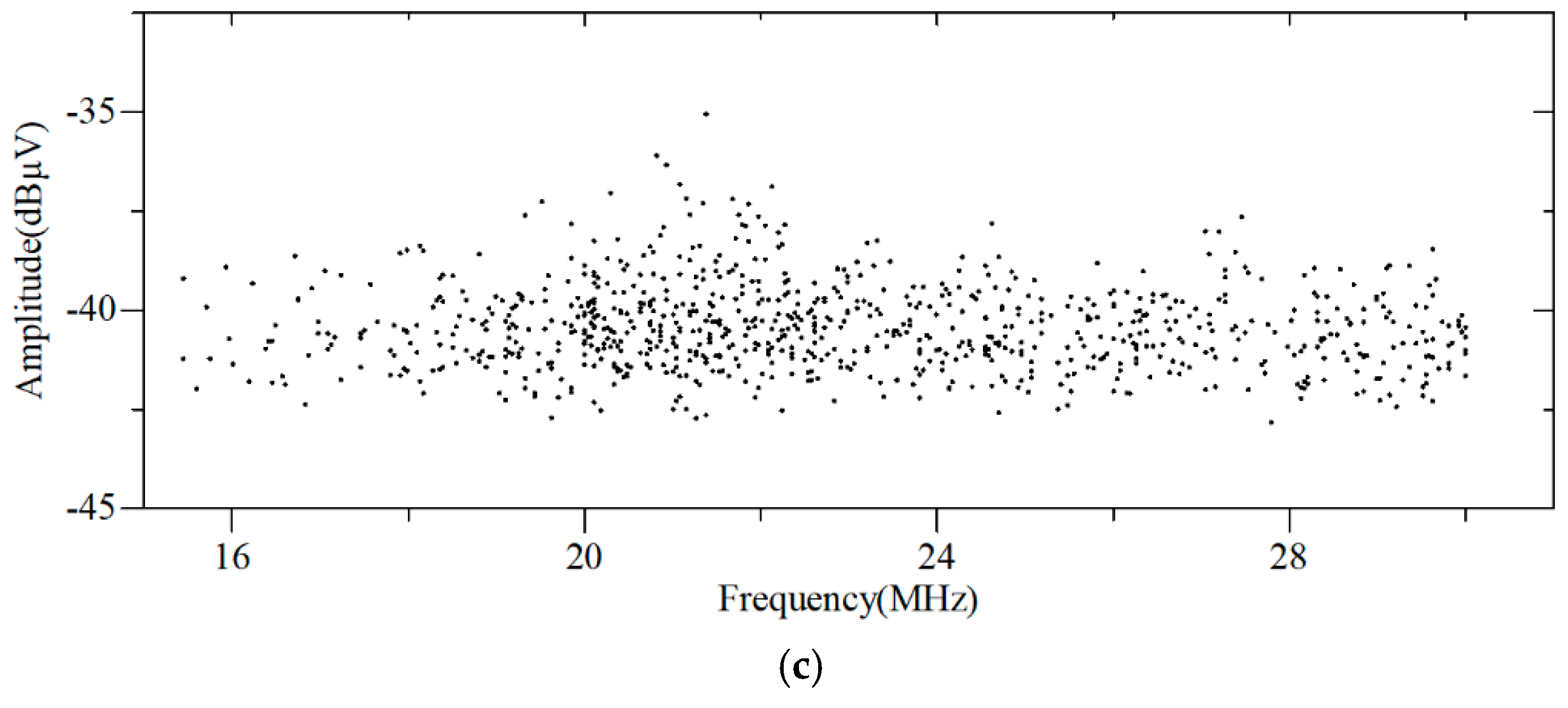
4.1. Distribution Diagram of Characteristic Points

$p_{\mathrm{suspect}\_j}\left(U_j,f_{\mathrm{suspect}\_j}\right)$ is the j-th characteristic point, where $U_j$ is the amplitude and $f_{\mathrm{suspect}\_j}$ is the frequency of $p_{\mathrm{suspect}\_j}\left(U_j,f_{\mathrm{suspect}\_j}\right)$. Suppose that there are z spectrograms in a group of FFT spectrum analysis results. The set of characteristic points is:

$$\left[p_{\mathrm{suspect}\_1}\left(U_1,f_{\mathrm{suspect}\_1}\right),\dots ,p_{\mathrm{suspect}\_j}\left(U_j,f_{\mathrm{suspect}\_j}\right),\dots ,p_{\mathrm{suspect}\_z}\left(U_z,f_{\mathrm{suspect}\_z}\right)\right]\left(1\le j\le z\right),$$

where ${\mathbf{U}}_{\mathrm{suspect}}$ is the set of amplitudes and ${\mathbf{U}}_{\mathrm{suspect}}=\left[U_1,\dots ,U_j,\dots ,U_z\right]$. ${\mathbf{F}}_{\mathrm{suspect}}$ is the frequency set and ${\mathbf{F}}_{\mathrm{suspect}}=\left[f_{\mathrm{suspect}\_1},\dots ,f_{\mathrm{suspect}\_j},\dots ,f_{\mathrm{suspect}\_z}\right]$.

Suppose that $p_{\max }\left(U_{\max },f_{\mathrm{U}\_\max }\right)$ is the characteristic point with maximum amplitude and $U_{\max }=\max \left\{{\mathbf{U}}_{\mathrm{suspect}}\right\}$. $p_{\min }\left(U_{\min },f_{U\_\min }\right)$ is the characteristic point with minimum amplitude and $U_{min}=\min \left\{{\mathbf{U}}_{\mathrm{suspect}}\right\}$.

A distribution diagram of characteristic points is shown in Figure 5 with the set of characteristic points. The abscissa is frequency, and the ordinate is amplitude.

4.2. EMI Evaluation Indexes for New Energy Vehicles under Dynamic Conditions

According to Figure 5, $p_{\max }\left(U_{\max },f_{\mathrm{U}\_\max }\right)$, area Π, point ratio η, and density coefficient ρ of high-amplitude characteristic points can be obtained. The physical significance is as follows:

(1) The characteristic point has a maximum amplitude $p_{\max }\left(U_{\max },f_{\mathrm{suspect}\_\max }\right)$ and a set of characteristic points, $U_{\max }=\max \left\{{\mathbf{U}}_{\mathrm{suspect}}\right\}$, then $f_{\mathrm{U}\_\max }$ can be found. $U_{\max }$ is an index to evaluate extreme values, indicating the maximum EMI value under these dynamic conditions. The larger $U_{\max }$ is, the larger the EMI value is, and the larger EMI that is generated by new energy vehicles.

(2) Area Π and point ratio η of high-amplitude characteristic points.

Area Π of high-amplitude characteristic points is the area with the amplitude higher than the threshold, $U_{\mathrm{T}}$. The amplitude range of the characteristic points in area Π is $\left[U_{\mathrm{T}},U_{\max }\right]$. Suppose that there are $N_{\Pi }$ characteristic points in area Π. Then, the ratio between $N_{\Pi }$ and the total number of characteristic points, z, is named point ratio η of high-amplitude characteristic points. η is calculated as:

$$\eta =N_{\Pi }/z.$$

(1)

When $U_{\mathrm{T}}$ is constant, the larger the η is, the larger the EMI that is generated at multiple frequencies by new energy vehicles. Π and η are comprehensive indexes to evaluate the overall region.

(3) Density coefficient ρ of high-amplitude characteristic points.

Set a rectangular shape area as a local observation area, ${\Pi }_f$, with left frequency boundary $f_{\mathrm{left}}$, frequency width w, lower amplitude boundary $U_{\mathrm{down}}$, and amplitude length l ($l=U_{\max }-U_{\mathrm{down}}$). The amplitude range of the characteristic points in area ${\Pi }_f$ is $\left[U_{\mathrm{down}},U_{\max }\right]$. The frequency range of the characteristic points in area ${\Pi }_f$ is $\left[f_{\mathrm{left}},f_{\mathrm{left}}+w\right]$. When $U_{\mathrm{down}}=U_{\mathrm{T}}$, suppose that there are N characteristic points in area ${\Pi }_f$. Then, the ratio between N and wl is named the density coefficient ρ of high-amplitude characteristic points. ρ is calculated as:

$$\rho =N/wl.$$

(2)

The total number of characteristic points z increases with time, resulting in N of the same condition and the same region also increases with time. ρ will be affected as different dynamic conditions have different durations. In order to compare the ρ among different dynamic conditions, condition duration t is introduced. The density per unit time ${\rho }_t$ is calculated as:

$${\rho }_t=\rho /t.$$

(3)

When $U_{\mathrm{down}}$ and w are constant ($U_{\mathrm{down}}=U_{\mathrm{T}}$), the larger the ρ is, the more EMI that is generated by new energy vehicles, indicating a greater EMI in this area. ρ is an index to evaluate local regions.

According to the definitions of $p_{\max }\left(U_{\max },f_{\mathrm{U}\_\max }\right)$, Π, η. and ρ, EMI evaluation indexes for new energy vehicle under dynamic conditions are shown in Figure 6.

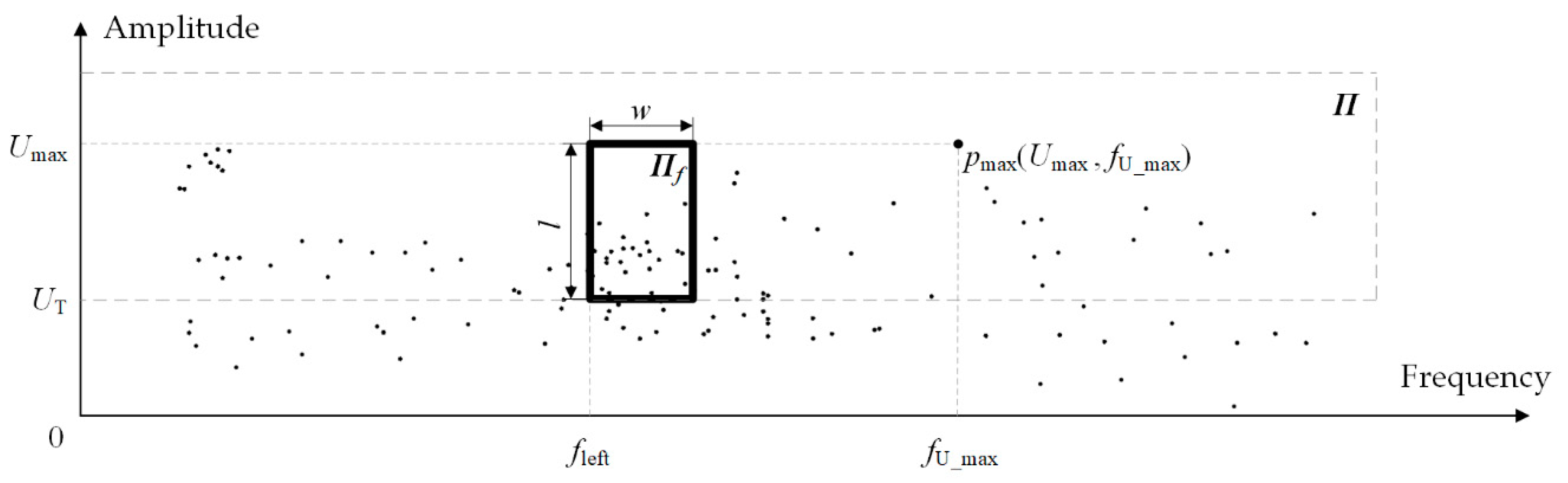
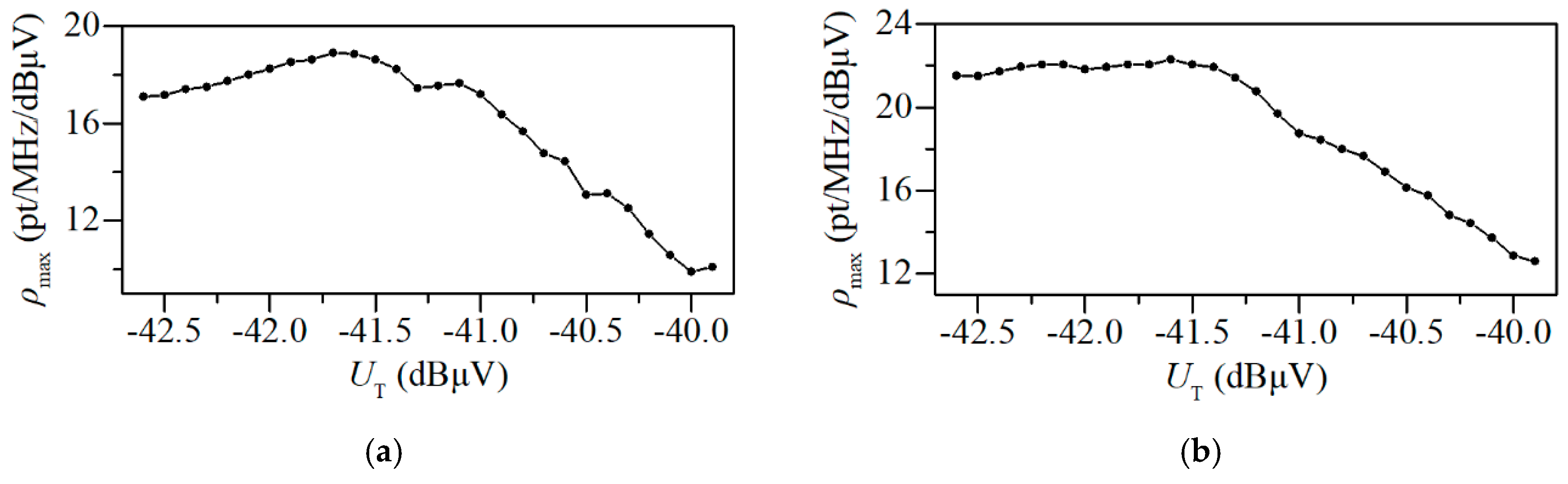
4.3. Method to Determine Characteristic Points Based on EMI Evaluation Indexes

A distribution diagram of characteristic points and EMI evaluation indexes is illustrated above. Now, the problem is that the frequency resolution’s accuracy from the FFT spectrum analysis is low. Searching all the characteristic points that effect EMI evaluation indexes the most in carrying out small frequency range FFT and DFS helps to improve accuracy of the frequency resolution.

$U_{\max }$ is an index to evaluate extreme values. Π and η are comprehensive indexes to evaluate the overall region. ρ is an index to evaluate the local region. $p_{\max }\left(U_{\max },f_{\mathrm{U}\_\max }\right)$ and ρ are EMI evaluation indexes that the characteristic points affect the most. Therefore, the method to determine characteristic points based on EMI evaluation indexes under dynamic conditions is as follows:

(1)

$p_{\max }\left(U_{\max },f_{\mathrm{U}\_\max }\right)$, where $U_{\max }=\max \left\{{\mathbf{U}}_{\mathrm{suspect}}\right\}$. $f_{\mathrm{U}\_\max }$ is a frequency concerned by the EMI test for new energy vehicles under dynamic conditions.

(2)

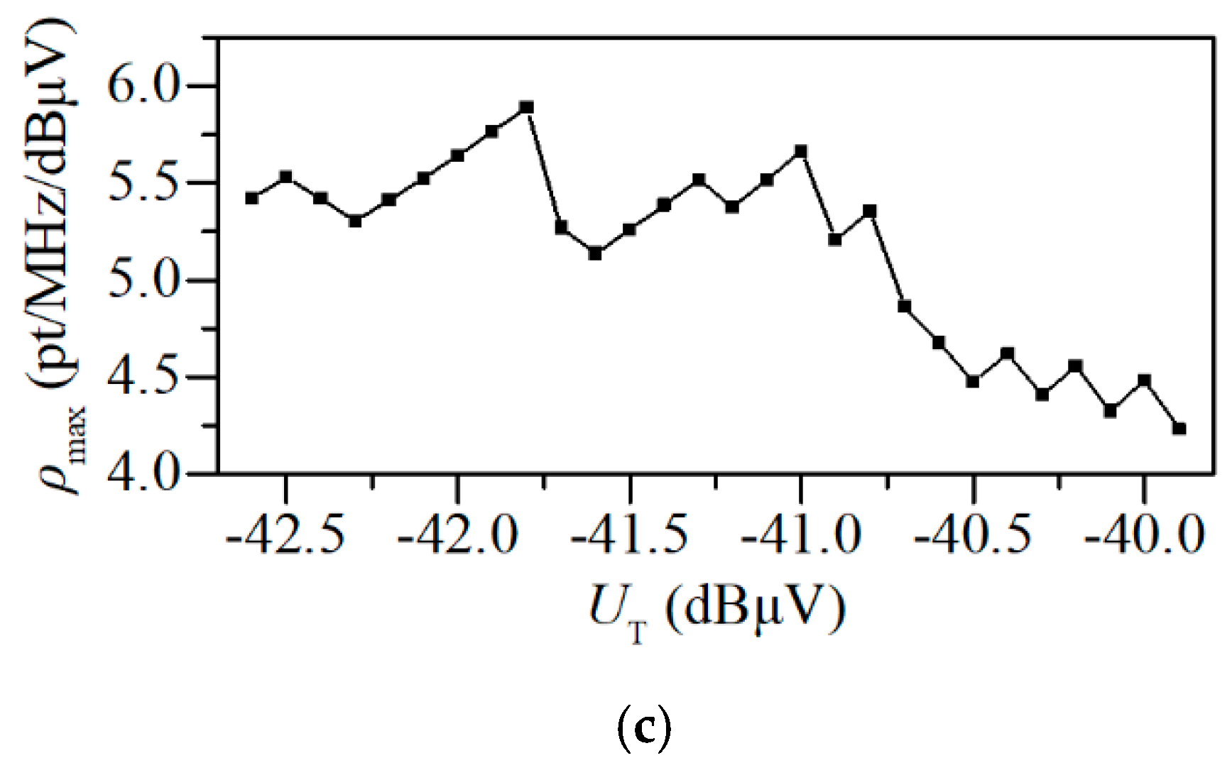
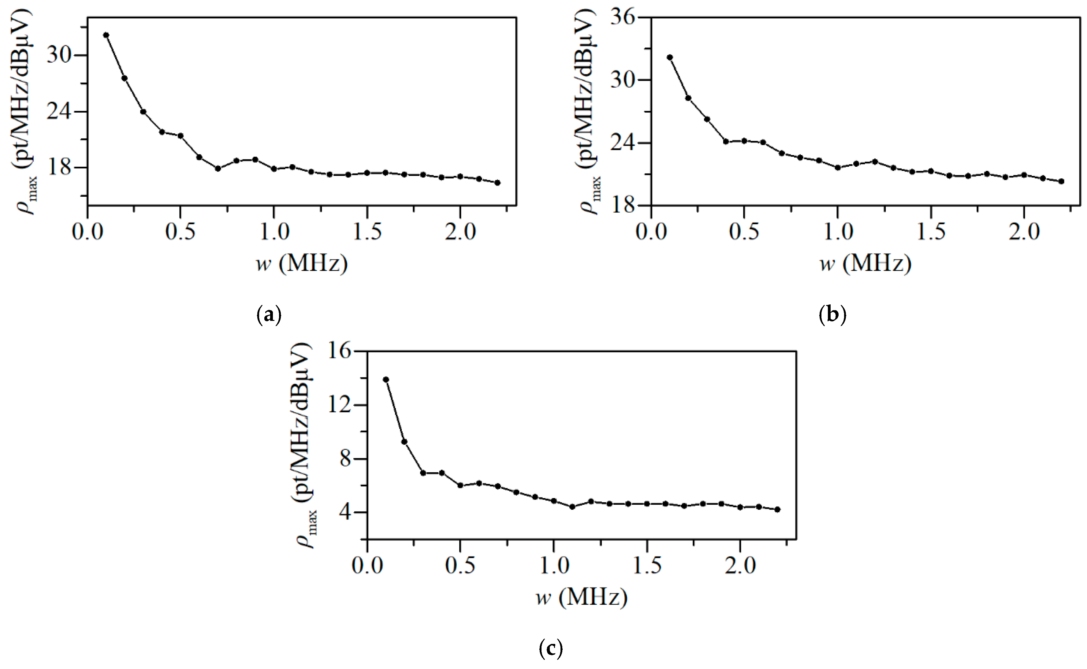
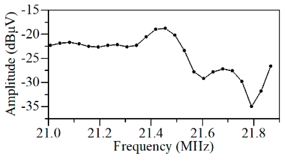
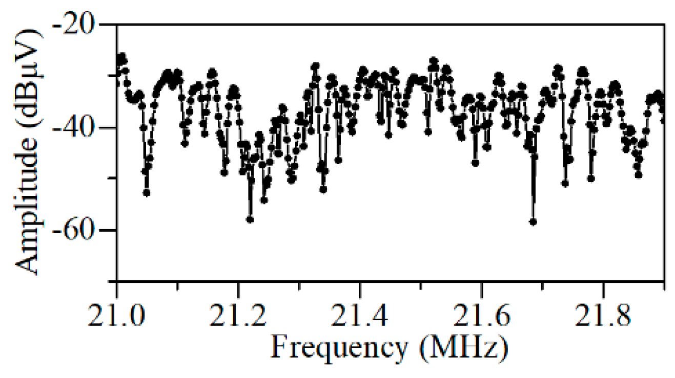
When $U_{\mathrm{down}}$ ($U_{\mathrm{down}}=U_{\mathrm{T}}$) and w are constant, the larger ρ is, the more EMI that is generated by new energy vehicles. Therefore, the frequencies in the area whose ρ is larger than the threshold (especially the area whose ρ is maximum) should be included in the EMI test for new energy vehicles under dynamic conditions.

5. Implementations and Experiments

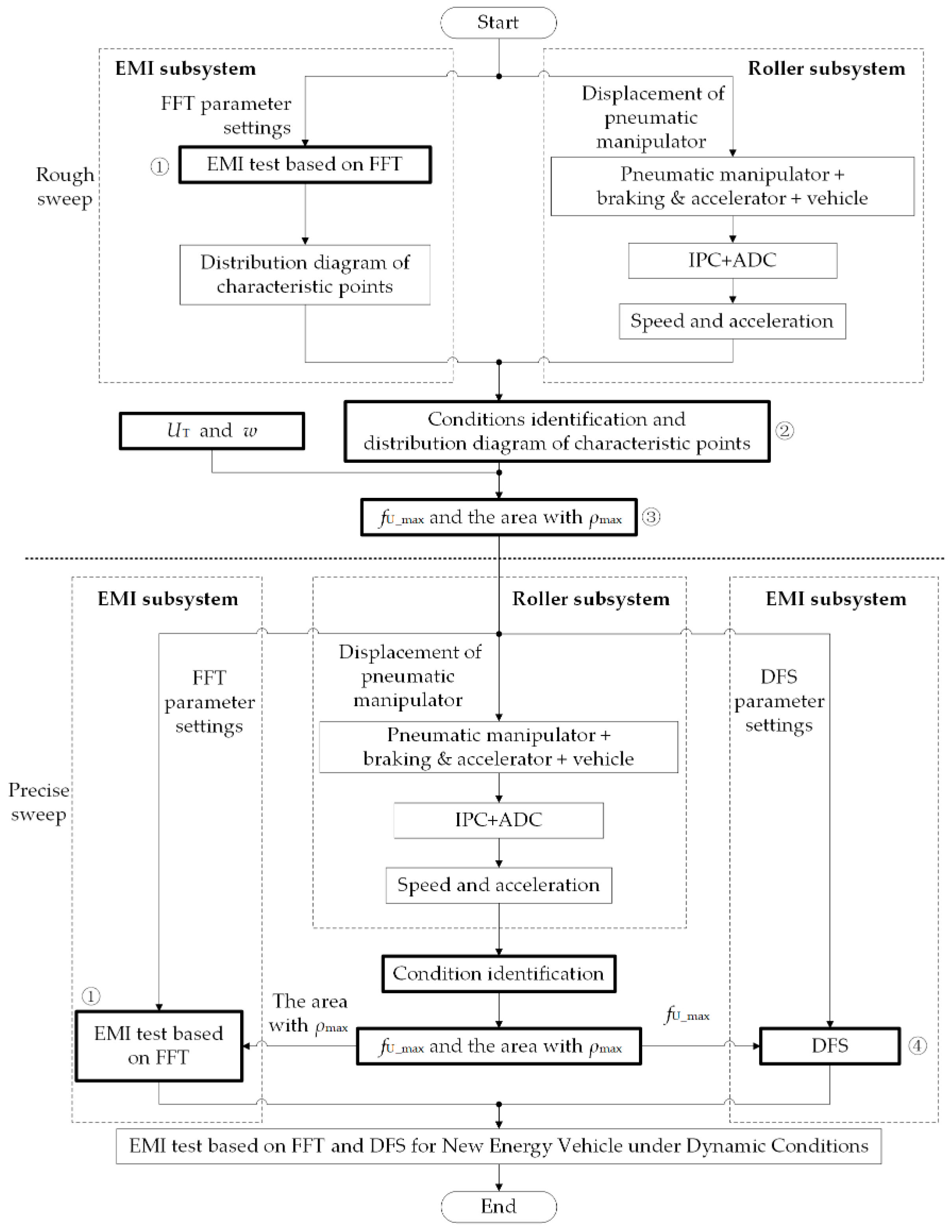
5.1. Implementation Flow

Based on the method to identify dynamic accelerating, sliding, and braking conditions, and to determine the characteristic points, EMI tests for new energy vehicles under dynamic conditions can be implemented. A flow chart of an EMI test based on FFT and DFS for new energy vehicles under dynamic conditions is shown in Figure 7, which mainly includes rough sweep based on FFT and precise sweep based on FFT and DFS. Firstly, rough sweep obtains a distribution diagram of the characteristic points under different dynamic conditions. Secondly, $p_{\max }\left(U_{\max },f_{\mathrm{U}\_\max }\right)$ and the area whose ρ is maximized are calculated. Finally, precise sweep takes place. In the second step, it is very important to select $U_{\mathrm{T}}$ and w reasonably.

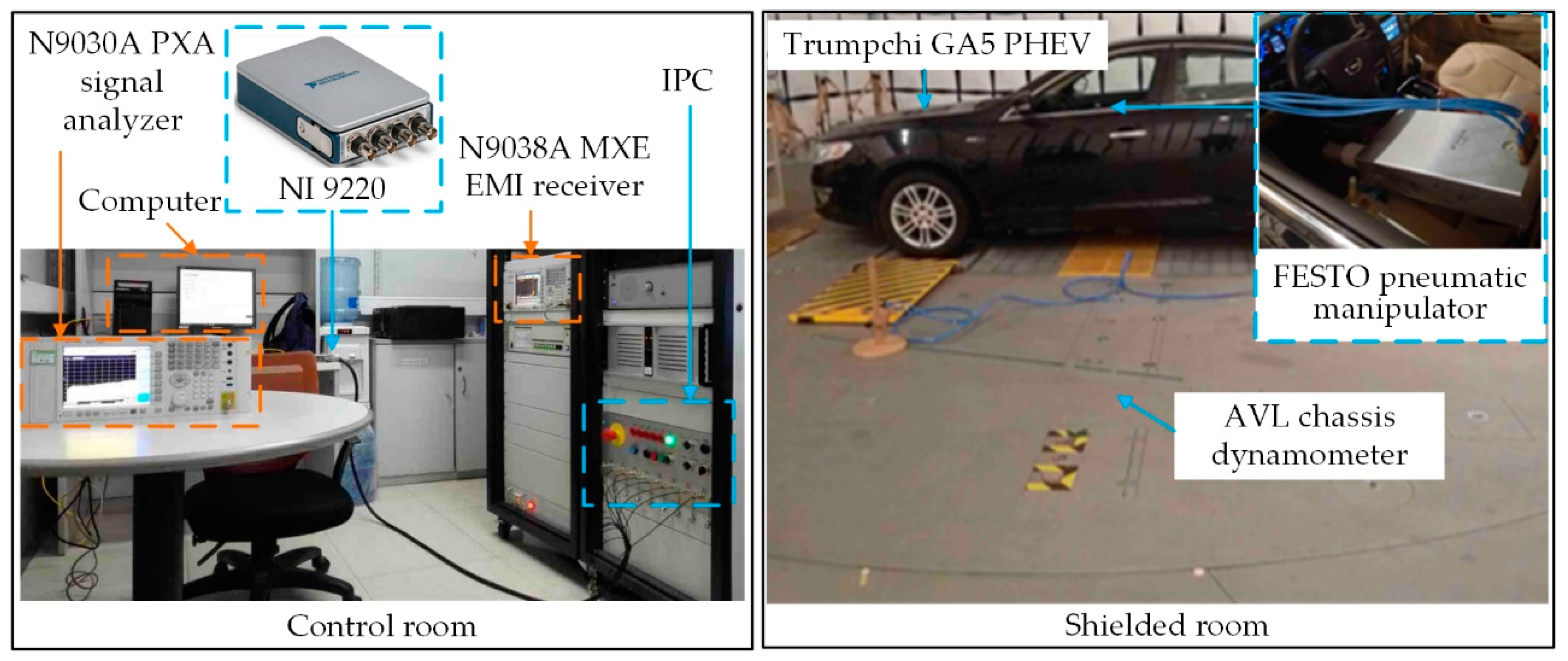
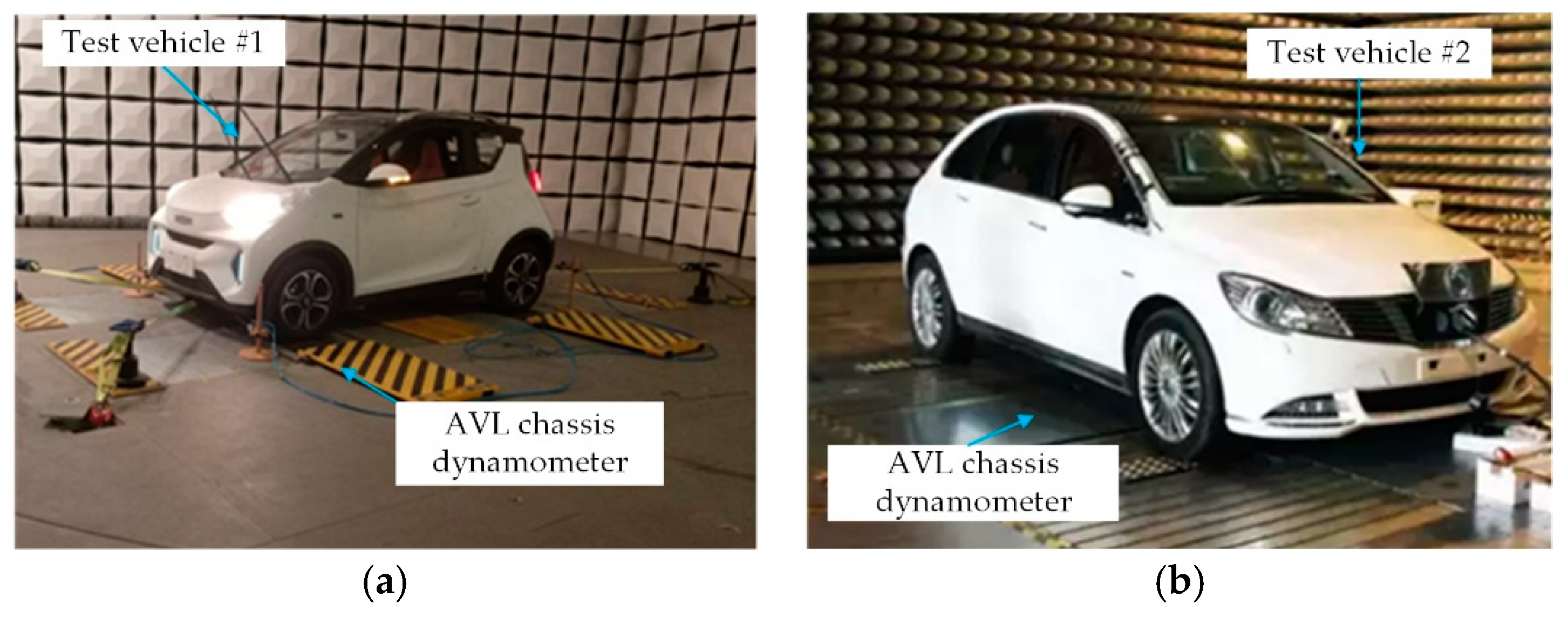
5.2. Construction of the Experimental System

According to Figure 1, the experimental system of the EMI test based on FFT and DFS for new energy vehicles under dynamic conditions was constructed, as shown in Figure 8. The whole system was arranged in a control room and a shielded room. The control room contained a signal analyzer, an EMI receiver, a computer from an EMI test subsystem, an IPC, and an ADC from a roller subsystem. The signal analyzer was N9030A PXA from Agilent. The EMI receiver was N9038A MXE from Agilent. The computer contained a B85-HD3-A board, an i7-4790K CPU, 16 GB RAM, and Windows 10 operating system. The velocity was transformed into voltage in the range from −10 to 10 V, which was outputted with a BNC on an IPC. The ADC was NI 9220 from National Instrument. The shielded room contained an antenna from the EMI test subsystem and a pneumatic manipulator, a test vehicle, and a chassis dynamometer from roller subsystem. The pneumatic manipulator was customized by Festo AG & Co. KG. GA5 PHEV produced by Guangzhou Automobile Group Co., Ltd., and the electric test vehicles of Zotye Auto Co., Ltd. and BYD Co., Ltd. were chosen. The chassis dynamometer was made by AVL List GmbH. Under the condition that the wheel and the roller do not slip relative to each other, the vehicle speed was equal to the linear speed of the roller. The roller could handle a range of velocity (0~200 km/h) in both front and reverse directions. Its velocity sensor had a range of accuracy of 0.05–0.1 km/h.

5.3. Experimental Process and Results

According to Section 5.1, three experiments were carried out: (1) An experiment to identify dynamic conditions verified the method. (2) A calculation experiment of $f_{\mathrm{U}\_\max }$ and the area with ${\rho }_{\max }$ under different dynamic conditions discussed the results depending on different $U_{\mathrm{T}}$ and w. (3) An experiment of the EMI test based on FFT and DFS verified the entire EMI test method and evaluated the accuracy of the measurements. Finally, the EMI test method based on FFT and DFS for new energy vehicles under dynamic conditions was applied to the electric test vehicles of Zotye Auto Co., Ltd. (Yongkang, China) and BYD Co., Ltd. (Shenzhen, China) to verify its effectiveness and applicability.

5.3.1. Experiments of GA5 PHEV

(1) The experiment to identify dynamic conditions.

The experiment to identify dynamic conditions used an FFT spectrum analysis to calculate EMI data at multiple frequencies. Then, a distribution diagram of characteristic points was obtained. According to the identification results of different dynamic conditions from speed and acceleration, different condition distribution diagrams of characteristic points were distinguished.

The experiment processes were as follows: The test vehicle was driven on the chassis dynamometer where the wheel and the roller coincide. The computer controlled the pneumatic manipulator to handle the vehicle and controlled the signal analyzer to measure EMI.

A group of EMI test results, based on FFT for new energy vehicles under dynamic conditions, is shown in Figure 9, where Figure 9a is the speed and acceleration curves, and Figure 9b is the EMI intensity graph. According to Table 1, when the condition $a_i\ge a_{\min }>a_{\mathrm{T}\_\mathrm{acc}}>0$ is detected, it indicates that the test vehicle is accelerating. When the conditions $v_{\mathrm{idling}}<v_{\min }\le v_i$ and $a_{\max }<-a_{\mathrm{T}\_\mathrm{slide}}$ are detected, it indicates that the test vehicle is sliding. When the condition $a_i\le a_{\max }<a_{\mathrm{slide}}-a_{\mathrm{T}\_\mathrm{brake}}<0$ is detected, it indicates that the test vehicle is braking. Based on experience, $a_{\mathrm{T}\_\mathrm{acc}}=a_{\mathrm{T}\_\mathrm{slide}}=0.1{\mathrm{m}/\mathrm{s}}^2$, $a_{\mathrm{T}\_\mathrm{brake}}=0.5{\mathrm{m}/\mathrm{s}}^2$, and $v_{\mathrm{idling}}=10\mathrm{km}/\mathrm{h}$. Then, the vehicle was identified to accelerate during 0~21.3 s, slide during 21.3~58.5 s, and brake during 90.0~96.2 s. It can be seen that the values of $a_{\mathrm{T}\_\mathrm{acc}}$, $v_{\mathrm{idling}}$, $a_{\mathrm{T}\_\mathrm{slide}}$, $a_{\mathrm{T}\_\mathrm{brake}}$ would affect the identification results.

EMI data of different conditions were obtained by combining the identification results and the EMI test results, which is shown in Figure 9b. According to Section 4.1, distribution diagrams of the characteristic points in different dynamic conditions are shown in Figure 10. All abscissas are frequency (MHz), and all ordinates are amplitude (dBμV). Figure 10a–c depicts distribution diagrams of characteristic points during acceleration, sliding, and braking, respectively.

Using the identification results to fit the EMI data, any dynamic condition distribution diagram of characteristic points can be obtained. The method to identify acceleration, sliding, and braking was correct and effective.

(2) Experimental calculation of $f_{\mathrm{U}\_\max }$ and the area with ${\rho }_{\max }$ under different dynamic conditions.

According to Section 4.2 and Section 4.3, $f_{\mathrm{U}\_\max }$ and the area with ${\rho }_{\max }$ under different dynamic conditions can be obtained from the distribution diagrams of characteristic points. $f_{\mathrm{U}\_\max }$ attracts great attention as the frequency corresponding to $U_{\max }$. According to Figure 10, $f_{\mathrm{U}\_\max }$ = $21.38\mathrm{MHz}$ under accelerating conditions. $f_{\mathrm{U}\_\max }=22.05\mathrm{MHz}$ under sliding conditions. $f_{\mathrm{U}\_\max }=21.49\mathrm{MHz}$ under braking conditions.

The area with ${\rho }_{\max }$ relates to the values of $U_{\mathrm{T}}$ and w. The analyses are as follows:

(1) Constant w and changing $U_{\mathrm{T}}$. Based on Figure 10, let $w=0.9\mathrm{MHz}$. The relationship between $U_{\mathrm{T}}$ and ${\rho }_{\max }$ is shown in Figure 11. Figure 11a–c is the relationship between $U_{\mathrm{T}}$ and ${\rho }_{\max }$ under accelerating, sliding, and braking conditions, respectively, when $-42.6\mathrm{dB}\mathsf{\mu }\mathrm{V}\le U_{\mathrm{T}}\le -39.9\mathrm{dB}\mathsf{\mu }\mathrm{V}$. It can be seen that different $U_{\mathrm{T}}$ values correspond to different ${\rho }_{\max }$ values. Among the curves in Figure 11, the maximum of ${\rho }_{\max }$, ${\rho }_{\max |\max }$, was 22.3 pt/MHz/dBμV when $U_{\mathrm{T}}=-39.9\mathrm{dB}\mathsf{\mu }\mathrm{V}$ under sliding conditions, and the minimum of ${\rho }_{\max }$, ${\rho }_{\max |\min }$, was 4.2 pt/MHz/dBμV when $U_{\mathrm{T}}=-41.6\mathrm{dB}\mathsf{\mu }\mathrm{V}$ under braking conditions. ${\rho }_{\max |\max }$ and ${\rho }_{\max |\min }$ were largely different. If ${\rho }_{\max }$ was too small, which means that there were few points per MHz and per dBμV, this area had no practical guidance. Therefore, $U_{\mathrm{T}}$ should be selected carefully when w is constant.

(2) Constant $U_{\mathrm{T}}$ and changing w. Based on Figure 10, let $U_{\mathrm{T}}=-41.6\mathrm{dB}\mathsf{\mu }\mathrm{V}$. The relationship between w and ${\rho }_{\max }$ is shown in Figure 12. Figure 12a–c is the relationship between w and ${\rho }_{\max }$ under accelerating, sliding, and braking conditions, respectively, when $0.1\mathrm{MHz}\le w\le 2.2\mathrm{MHz}$.

It can be seen that different w values correspond to different ${\rho }_{\max }$ values. ρ is an index to evaluate local regions, reflecting the level of EMI generated by new energy vehicles. When $w\to 0$, ${\rho }_{\max }$ would be much larger but has little practical guidance.

Therefore, it is reasonable that $U_{\mathrm{T}}=-41.6\mathrm{dB}\mathsf{\mu }\mathrm{V}$ and $w=0.9\mathrm{MHz}$. The ${\rho }_{\max }$ and the frequency range when $U_{\mathrm{T}}=-41.6\mathrm{dB}\mathsf{\mu }\mathrm{V}$ and $w=0.9\mathrm{MHz}$ under different conditions are shown in

Table 2. The ${\rho }_{\max }$ and the frequency range when $U_{\mathrm{T}}=-41.6\mathrm{dB}\mathsf{\mu }\mathrm{V}$ and $w=0.9\mathrm{MHz}$.

Parameter	Acceleration	Sliding	Braking
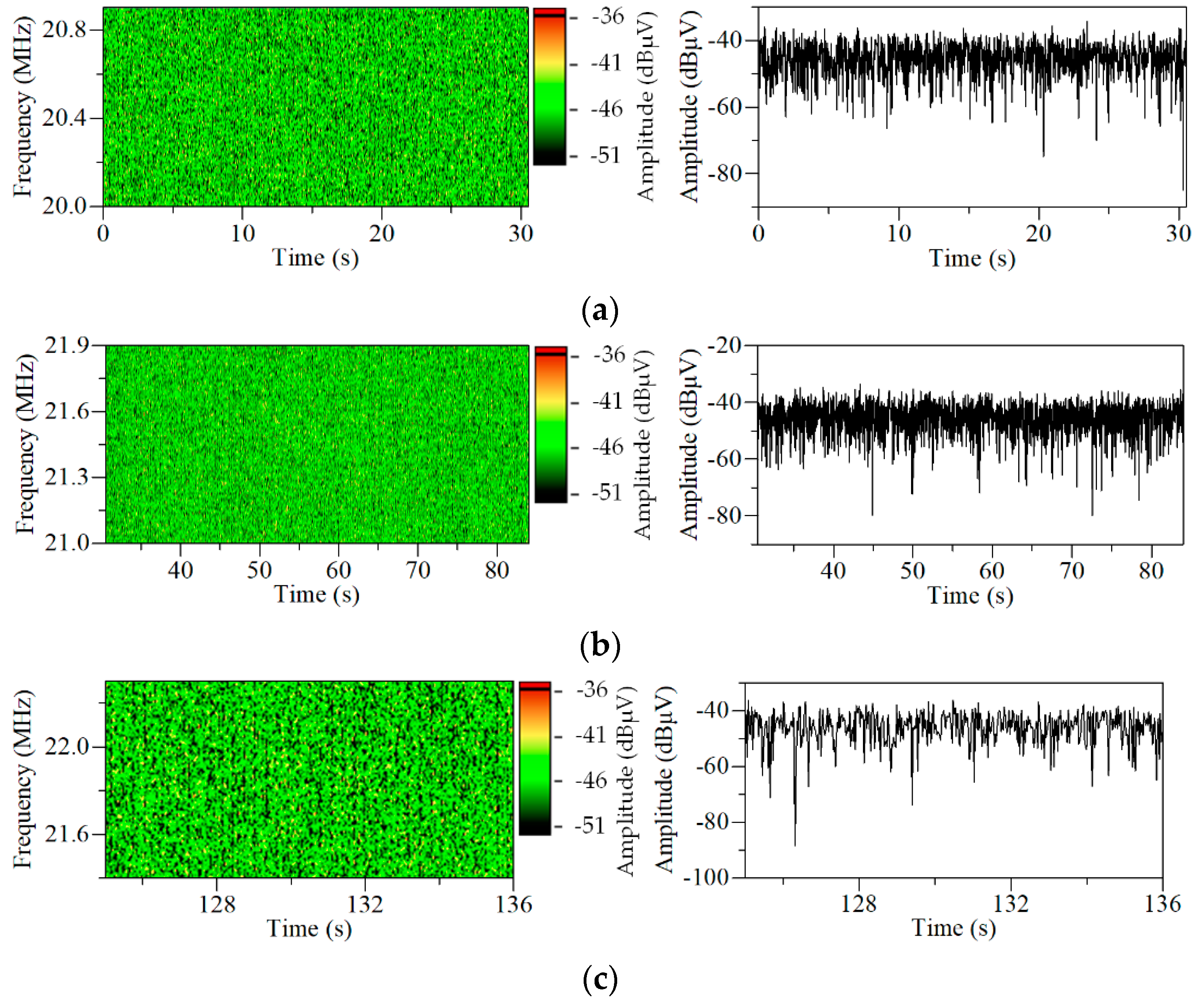
${\rho }_{\max }$ (pt/MHz/dBμV)	18.9	22.3	5.1
The frequency range of the area with ${\rho }_{\max }$ (MHz)	20.0~20.9	21.0~21.9	21.4~22.3

.

(3) EMI experimental test based on FFT and DFS.

The experimental EMI test based on FFT and DFS identifies accelerating, sliding, and braking conditions in real time from the speed and acceleration. Meanwhile, it uses DFS to measure the EMI of $f_{\mathrm{U}\_\max }$ and uses FFT spectrum analyses to measure the EMI of ${\rho }_{\max }$ area. The specific experimental ideas are analyzed as follows.

(1) In the experiment of the EMI test based on FFT and DFS, the FFT frequency span $f_{\mathrm{span}}=w=0.9\mathrm{MHz}$, the frequency resolution $f_{\mathrm{resolution}}=2.5\mathrm{kHz}$, and the frequency accuracy $f_{\mathrm{accuracy}}=\pm 3.7\mathrm{kHz}$. In the dynamic conditions identification experiment, the FFT frequency span $f_{\mathrm{span}}=29.85\mathrm{MHz}$, the frequency resolution $f_{\mathrm{resolution}}=37.3\mathrm{kHz}$, and the frequency accuracy $f_{\mathrm{accuracy}}$ = $\pm 57.5\mathrm{kHz}$. Therefore, by reducing $f_{\mathrm{span}}$, $f_{\mathrm{resolution}}$ and $f_{\mathrm{accuracy}}$ were greatly improved with the same instruments.

(2) When the vehicle was accelerating, the FFT spectrum analysis was applied from 20.0 to 20.9 MHz with ±1.31 dB amplitude accuracy, and DFS was applied to $f_{\mathrm{U}\_\max }=21.38\mathrm{MHz}$ with ±0.36 dB amplitude accuracy. When the vehicle was sliding, the FFT spectrum analysis was applied from 21.0 to ~21.9 MHz with ±1.31 dB amplitude accuracy, and DFS was applied to $f_{\mathrm{U}\_\max }=22.05\mathrm{MHz}$ with ±0.36 dB amplitude accuracy. When the vehicle was braking, the FFT spectrum analysis was applied to 21.4 to ~22.3 MHz with ±1.31 dB amplitude accuracy, and DFS was applied to $f_{\mathrm{U}\_\max }=21.49\mathrm{MHz}$ with ±0.36 dB amplitude accuracy.

The experiment of the EMI test based on FFT and DFS was similar to the dynamic conditions identification experiment, with the difference that an EMI receiver was added to measure EMI.

A group of condition identification results of the EMI test based on FFT and DFS is shown in Figure 13. According to Table 1 and experience, $a_{\mathrm{T}\_\mathrm{acc}}=a_{\mathrm{T}\_\mathrm{slide}}=0.1{\mathrm{m}/\mathrm{s}}^2$, $a_{\mathrm{T}\_\mathrm{brake}}=0.5{\mathrm{m}/\mathrm{s}}^2$, and $v_{\mathrm{idling}}=10\mathrm{km}/\mathrm{h}$. Then, the vehicle can be identified that it was accelerating from 0 to 30.5 s, sliding from 30.5 to 84.0 s, and braking from 125.0 to 136.0 s.

A group of EMI intensity graphs in ${\rho }_{\max }$ area and $f_{\mathrm{U}\_\max }$ amplitude are shown in Figure 14, where Figure 14a–c depicts the EMI intensity graph in ${\rho }_{\max }$ area and $f_{\mathrm{U}\_\max }$ amplitude under accelerating, sliding, and braking conditions.

A spectrogram of EMI test results based on FFT from 21.0 to 21.9 MHz with $f_{\mathrm{span}}=30\mathrm{MHz}$ is shown in Figure 15. A spectrogram of EMI test results based on FFT and DFS from 21.0 to 21.9 MHz with $f_{\mathrm{span}}=0.9\mathrm{MHz}$ is shown in Figure 16. It can be seen that there are 24 points in Figure 15 with 37.3 kHz frequency resolution and 361 points with 2.5 kHz frequency resolution in Figure 16. Therefore, $f_{\mathrm{resolution}}$ can be significantly improved by reducing $f_{\mathrm{span}}$.

5.3.2. Test Results of Other Test Vehicles

In order to prove the applicability and effectiveness of the method on different vehicles, the EMI test method, based on FFT and DFS for new energy vehicle under dynamic conditions, was applied to the electric test vehicles of Zotye Auto Co., Ltd. (hereinafter referred to as “test vehicle #1”) and BYD Co., Ltd. (hereinafter referred to as “test vehicle #2”). Figure 17 shows the test sites of the vehicles.

A group of EMI test results based on FFT for test vehicles under dynamic conditions is shown in Figure 18, where Figure 18a is the result of test vehicle #1, and Figure 18b is the result of test vehicle #2.

Table 3. EMI evaluation indexes for different conditions of the test vehicles (The numerical value in the boxes is emphasized).

Parameter	Test Vehicle #1			Test Vehicle #2
	Accelerating (0~9.3 s)	Sliding (17.7~33.7 s)	Braking (12.5~17.7 s)	Accelerating (0s~35 s)	Sliding (35~62 s)	Braking (90~97 s)
$f_{\mathrm{U}\_\max }$ (MHz)	29.59	20.10	29.51	16.66	16.85	16.78
$U_{\max }$ (dBμV)	−32.54	−32.94	−30.51	−2.72	−7.82	−6.86
η	0.78	0.67	0.90	0.94	0.87	0.87
The frequency range of the area with ${\rho }_{\max }$ (MHz)	29.0~30.0	20.1~21.1	29.0~30.0	19.8~20.8	20.0~21.0	16.5~17.5
${\rho }_{\max }$/t (pt/MHz/dBμV/min)	91.6	30.8	132.7	32.1	27.8	48.9

shows the EMI evaluation indexes for different conditions of the test vehicles. The numerical value in the boxes are emphasized. EMI tests based on FFT and DFS for test vehicles under dynamic conditions were carried out according to the EMI evaluation indexes. Figure 19 and Figure 20 are test results of test vehicle #1 and test vehicle #2.

The following can be seen from Table 3:

(1) The $f_{\mathrm{U}\_\max }$ values of test vehicle #1 under accelerating, sliding, and braking conditions were 29.59, 20.10, and 29.51 MHz. The $f_{\mathrm{U}\_\max }$ values of test vehicle #2 under accelerating, sliding, and braking conditions were 16.66, 16.85, and 16.78 MHz, which were lower than the $f_{\mathrm{U}\_\max }$ values of test vehicle #1. However, the $U_{\max }$ of test vehicle #1 under different conditions was smaller than the $U_{\max }$ of test vehicle #2. Therefore, as for the index to evaluate extreme values, $U_{\max }$, the EMI performance of test vehicle #1 was better than that of test vehicle #2.

(2) The point ratio η of test vehicle #1 under braking conditions was 0.90. The point ratio η of test vehicle #2 under accelerating conditions was 0.94. This indicates that there were many characteristic points exceeding the respective $U_{\mathrm{T}}$. As for the comprehensive index to evaluate the overall region, η, it was necessary to pay special attention to the characteristic points under braking conditions of test vehicle #1 and accelerating conditions of test vehicle #2.

(3) The maximum ${\rho }_t$ (29.0~30.0 MHz) of test vehicle #1 was 132.7 pt/MHz/dBμV/min under braking conditions. The maximum ${\rho }_t$ (16.5~17.5 MHz) of test vehicle #2 under braking conditions was 48.9 pt/MHz/dBμV/min. As for the index to evaluate the local region ${\rho }_t$, it was necessary to pay attention to the concentrated characteristic points between 29.0 and 30.0 MHz of test vehicle #1 and the characteristic points between 16.5 and 17.5 MHz of test vehicle #2 under braking conditions.

Through the EMI test based on FFT and DFS for test vehicles under dynamic conditions, the dynamic conditions can be identified. And the dynamic EMI can be measured with higher accuracy. The harshest cases can be judged from $U_{\max }$. The amplitude range of characteristic points can be judged from η. The regions with concentrated characteristic points can be judged from ${\rho }_t$. These help us to evaluate and improve the vehicle’s EMI performance.

5.4. Comparison Among Different EMI Test Methods

The results of different EMI test methods are shown in Figure 21. Figure 21a–d depicts the test results from previous studies [12,13,14] and this paper. We marked the elements with numbers as follows: (1) driving conditions (e.g., speed/torque); (2) frequency span; (3) amplitude; (4) time; and (5) characteristic points. Figure 21a includes driving conditions, amplitude and time, which constitute the result of DFS. Figure 21b includes frequency span and amplitude, which constitute the result of frequency sweeping. Figure 21c includes frequency span, amplitude, and time, which constitute the result of FFT. The test results of this paper shown in Figure 21d include elements (1)–(4). In addition, characteristic points were calculated out for more precise measurement.

6. Conclusions and Prospects

This paper proposes an EMI test method based on FFT and DFS for new energy vehicles under dynamic conditions, which makes full use of FFT’s rapidity and DFS’s accuracy to effectively expand their applications, making EMI testing under dynamic conditions possible.

Based on the features of accelerating, sliding, and braking conditions, a method to identify accelerating, sliding, and braking conditions was proposed. Different dynamic conditions can be identified from any group of speed and acceleration curves, realizing the automation of identifying dynamic conditions during vehicle the measurement process.

A comprehensive EMI key evaluation index system for new energy vehicles was built, including characteristic points of maximum amplitude $p_{\max }\left(U_{\max },f_{\mathrm{suspect}\_\max }\right)$, area Π, ratio η, and density coefficient ρ of high-amplitude characteristic points. $U_{\max }$ is an index to evaluate extreme values. η is a comprehensive index to evaluate the overall region. And ρ is an index to evaluate the local region. The calculation formula of each index is deduced, while the physical significance of each index is expounded.

The EMI test method, based on FFT and DFS for new energy vehicle under dynamic conditions, was applied to GA5 PHEV, produced by Guangzhou Automobile Group Co., Ltd., and the electric test vehicles of Zotye Auto Co., Ltd. and BYD Co., Ltd. The results indicate that the EMI of new energy vehicles can be tested under dynamic conditions with high accuracy, and the evaluation indexes are operable. With the same instruments, by reducing $f_{\mathrm{span}}$ from 29.85 to 0.9 MHz, $f_{\mathrm{resolution}}$ improves from 37.3 to 2.5 kHz, and $f_{\mathrm{accuracy}}$ improves from $\pm 57.5\mathrm{kHz}$ to $\pm 3.7\mathrm{kHz}$. DFS is used in the EMI test with a ±0.36 dB amplitude accuracy.

In the future, more experiments will be carried out to develop EMI test standards and specifications for new energy vehicles under dynamic conditions.

References

- Yan, L.; Zhang, Y.; He, Y.; Gao, S.; Zhu, D.; Ran, B.; Wu, Q. Hazardous traffic event detection using Markov Blanket and sequential minimal optimization (MB-SMO). Sensors 2016, 16, 1084. [Google Scholar] [CrossRef]
- Yuan, X.; Liu, X.; Zuo, J. The development of new energy vehicles for a sustainable future: A review. Renew. Sustain. Energy Rev. 2015, 42, 298–305. [Google Scholar] [CrossRef]
- Wang, Q.; Liu, Q. Estimation of parasitic parameters and EMI improvement of a full-bridge PWM converter system in the electric vehicle. Electron. World 2016, 122, 24–29. [Google Scholar]
- CISPR 12:2009. Vehicles, Boats and Internal Combustion Engines—Radio Disturbance Characteristics—Limits and Methods of Measurement for the Protection of off-Board Receivers; Council of Standards Australia: Sydney, Australia, 2009. [Google Scholar]
- ECE 10.05. Uniform Provisions Concerning the Approval of Vehicles with Regard to Electromagnetic Compatibility; The United Nations Economic Commission for Europe: Geneva, Switzerland, 2014. [Google Scholar]
- SAE J551-5-2012. Performance Levels and Methods of Measurement of Magnetic and Electric Field Strength from Electric Vehicles, 150 kHz to 30 MHz; Society of Automotive Engineers: New York, NY, USA, 2012. [Google Scholar]
- GB/T 18387-2017. Limits and Test Method of Magnetic and Electric Field Strength from Electric Vehicles; Standardization Administration of the People’s Republic of China: Beijing, China, 2017.
- Zeng, B.; Deng, J.; Lin, D.; Lin, Q.; Liu, G. Comparison of below 30 MHz electric vehicle EMI measurements method standard. China Meas. Test 2016, 42, 11–14. [Google Scholar] [CrossRef]
- Guo, Y.; Wang, L.; Liao, C. Modeling and Analysis of Conducted Electromagnetic Interference in Electric Vehicle Power Supply System. Prog. Electromagn. Res. 2013, 139, 193–209. [Google Scholar] [CrossRef]
- Tondato, F.; Bazzell, J.; Schwartz, L.; Mc Donald, B.W.; Fisher, R.; Anderson, S.S.; Galindo, A.; Dueck, A.C.; Scott, L.R. Safety and interaction of patients with implantable cardiac defibrillators driving a hybrid vehicle. Int. J. Cardiol. 2016, 227, 318–324. [Google Scholar] [CrossRef] [PubMed]
- Chun, Y.; Park, S.; Kim, J.; Kim, H.; Hwang, K.; Kim, J.; Ahn, S. Electromagnetic Compatibility of Resonance Coupling Wireless Power Transfer in On-Line Electric Vehicle System. IEICE Trans. Commun. 2014, 2, 416–423. [Google Scholar] [CrossRef]
- Jeschke, S.; Hirsch, H. Investigations on the EMI of an electric vehicle traction system in dynamic operation. In Proceedings of the 2014 International Symposium on Electromagnetic Compatibility (EMC Europe), Gothenburg, Sweden, 1–4 September 2014; pp. 420–425. [Google Scholar]
- Peng, H.; Hu, J.; Jiang, C.; Liu, Q.; Xu, H.; He, Z. Analysis for the EMI measurement and propagation path in Hybrid Electric Vehicle. In Proceedings of the 1st IEEE Information Technology, Networking, Electronic and Automation Control Conference (ITNEC), Chongqing, China, 20–22 May 2016; pp. 1087–1090. [Google Scholar]
- Vassilev, A.; Ferber, A.; Wehrmann, C.; Pinaud, O.; Schilling, M.; Ruddle, A.R. Magnetic Field Exposure Assessment in Electric Vehicles. IEEE Trans. Electromagn. Compat. 2015, 57, 35–43. [Google Scholar] [CrossRef]
- Zhong, S.; Huang, J.; Wu, J.; Jiang, C.; Liu, G. Frame design and key technical analysis of EMI test system for new energy vehicle dynamic condition. China Meas. Test 2017, 8, 76–79. [Google Scholar]