Magnetohydrodynamics Stagnation-Point Flow of a Nanofluid Past a Stretching/Shrinking Sheet with Induced Magnetic Field: A Revised Model

Abstract

The revised Buongiorno’s nanofluid model with the effect of induced magnetic field on steady magnetohydrodynamics (MHD) stagnation-point flow of nanofluid over a stretching or shrinking sheet is investigated. The effects of zero mass flux and suction are taken into account. A similarity transformation with symmetry variables are introduced in order to alter from the governing nonlinear partial differential equations into a nonlinear ordinary differential equations. These governing equations are numerically solved using the bvp4c function in Matlab solver, a very adequate finite difference method. The influences of considered parameters ($Pr$, M, $\chi$, $Le$, $Nb$, $Nt$, S, and $\lambda$) on velocity, induced magnetic, temperature, and concentration profiles together with the reduced skin friction and heat transfer rate are discussed. Results from these criterion exposed the existence of dual solutions when magnetic field and suction are applied for a specific range of $\lambda$. The stability of the solutions obtained is carried out by performing a stability analysis.

1. Introduction

In preceding decades, a very active topic of studies continues to be the study of fluid flow and heat transfer past a stretching/shrinking surface. Although a large sum of works have made remarkable contributions to the development of the theory, a proportionally good amount of efforts have also been dedicated to daily engineering applications that include electronic equipment, thermal energy storage systems, glass-fiber manufacturing, wire drawing, paper milling, and extraction of polymer sheets (see Fisher [1]). As a matter of fact, stretching confers a unidirectional orientation to the extrudate, thereby improving its mechanical properties as the features of the end product are substantially influenced by the rate of cooling. Correspondingly, it is crucial to meticulously control the fluid and heat transfer mechanism as the desired quality of the final product relies heavily on the cooling procedure. Following the famous works of Tsou et al. [2], Sakiadis [3], and that of Crane [4] in spearheading the stretching sheet problem with boundary layer approximation, several similar studies have arose, emphasizing on the shrinking sheets aspect (see Miklavčič and Wang [5] and Wang [6]). The general deduction in previously reported manuscripts suggested that the shrinking/stretching is linearly proportional to the axial distance. The solution approach somehow leaves behind uncertainties pertaining the uniqueness of the solution.

The concept of magnetohydrodynamics (MHD), which analyses the performance of magnetically induced nanofluids in various boundary-layer flow control systems can be integral in the theoretical and experimental studies of fluid flow and heat transfer. Several instances where MHD concept is fundamentally applicable encompass nuclear reactor engineering, plasma studies, geothermal energy harvesting, polymer development, metallurgy, and MHD heat/mass transfer systems of which the details can be found in the books by [7,8,9], and in the classical papers such as [10,11,12,13]. Gul et al. [14] has stressed that the polarization is very powerful and the process persists even when the magnetic flux was eliminated entirely. Stimulus in the research of MHD stems contribute to diverse profitable applications in oil and gas sectors, solving geophysical problems, and agricultural engineering. In addition, the effects of magnetic flux on electrically conducting liquid consequently influences the efficiency of industrial equipment like bearings, MHD generators, and pumps. The versatility of MHD concept also means that it can be implemented in medical sector such as in tumors ablation, wound treatment, gastric medications, and sanitization of apparatus [15,16,17]. Tashtoush and Magableh [18] studied the blood flow in multi-stenosis arteries and discovered that the introduction of magnetic flux could alter the flow patterns. Mukhopadhyay [19] investigated MHD boundary layer flow in the presence of thermal stratification and concluded that the higher magnetic parameter suppressed the velocity field and can enhance the skin friction coefficient over some period of time. A similar output was acquired by Tian et al. [20], who explored the effects of radiation optical properties and Lorentz force on MHD boundary layer flow over a stretching plate. They explained that the magnetic force repressed the fluid flow to a significant magnitude, hence, the convective heat transfer was eliminated effectively. An equally notable paper by Ali et al. [21] presented a study of dual solutions in MHD flow on a nonlinear porous shrinking sheet in a viscous fluid, while another distinct paper by Jusoh et al. [22] emphasized the MHD rotating flow and permeable stretching/shrinking sheet. On the other hand, it should be mentioned that in these papers, Ali et al. [23,24] has studied the effect of induced magnetic field on the MHD flow of an incompressible, viscous, and electrically conducting fluid over horizontal and vertical flat plates.

Nanotechnology has been broadly applied in varying industries since nanomaterials possess distinctive physicochemical properties. It is regarded by many as one of the prominent forces that catalyze the forth industrial revolution, especially in this century. It appears that Choi and Eastman [25] are probably the first authors to describe the term nanofluid, referring to the colloid-containing suspended nanoparticles with a length scale on the order of 1–100 nm which specializes at manipulating the structure of the matter at a molecular level. For applications in thermal engineering, heat conductivity can be powered up by mixing a minute quantity of nanoparticles to a fluid. Several experimental studies [26,27,28,29,30] have shown that the enhancement is greater than that computed from the conventional models for composites, such as the Maxwell-Garnett (MG) model. However, the mechanism that contributes to the improvement is not thoroughly perceived, henceforth, a large number of analytical and numerical investigations have been put into motion to better comprehend the phenomena. These next-generation nanofluids can be implemented in various heat transfer applications such as automotive cooling systems, solar collector panels, and heat exchangers. Titanium oxide, aluminum oxide, and copper are among the archetypal nanoparticles used in nanofluid-centered research. Additionally, ethylene glycol, water, and mineral oil are often used as a base fluid in nanofluids formulation. For example, Bondareva et al. [31] have considered alumina-water nanofluid in their study. A detailed review on the application of nanofluids can be found in Saidur et al. [32]. References on nanofluids can be found in the book by [33,34,35,36] and in the review papers by [37,38,39,40,41,42,43]. These reviews discuss in detail the development of nanofluids, theoretical and experimental investigations of rheological properties (thermal conductivity and viscosity) of nanofluids, and the work done on convective transport in nanofluids. It would also be interesting to mention the study of hybrid nanofluid, which is one of the new classifications of nanofluid by Sheikholeslami et al. [44].

Over the past few decades, an impressive number of studies have demonstrated the presence of dual solutions in the boundary layer flow problems. There are few considerations that contribute to dual solutions such as a moving, stretching, or shrinking plate, mixed convection, permeable surface, where suction is an existent and unsteady case. For those interested in engineering analysis, the idea of discovering dual solutions and defining stability is of practical significance, as it offers a way to determine if a steady state solution is physically relevant [45]. This kind of research is therefore very useful in determining the dual solutions of fluid flow problems. Here, the work of Hussaini and Lakin [46] is worth mentioning among the pioneering researchers who discovered the uniqueness of solutions in the boundary layer problems. Magyari et al. [47] has presented dual solutions in homogenous boundary layer flows caused by continuous surface stretching with rapidly decreasing power-law and exponential velocities. Subsequently, in unsteady cases, Merrill et al. [48] studied the mixed stagnation-point convection flow on a vertical surface in a fluid-saturated porous medium and discovered that there exist dual solutions for certain buoyancy parameter values. By conducting a stability analysis by Merkin [49], Merrill et al. [48] demonstrated that the solutions of the upper branch are stable and therefore asymptotically available solutions. Very recently, the effect of induced magnetic field on MHD stagnation-point flow of nanofluids towards stretching/shrinking sheet was analyzed by Junoh et al. [50]. Since the existence of dual solutions for a certain range of shrinking rate, a stability analysis has been performed and the result showed that only the upper branch solution is stable and physically acceptable.

The purpose of this present paper is to extend the work by Junoh et al. [50] by considering the presence of suction on MHD stagnation-point flow of heat and mass transfer over a permeable stretching/shrinking sheet in a nanofluid. The effect of induced magnetic field is also taken into account. In this study, the new boundary condition proposed by Kuznetsov and Nield [51] will be implemented. This work also highlights the stability of the solutions obtained. Therefore, we presume the findings are new and original, which all those interested in stretching/shrinking sheet problems in nanofluids can use with strong confidence.

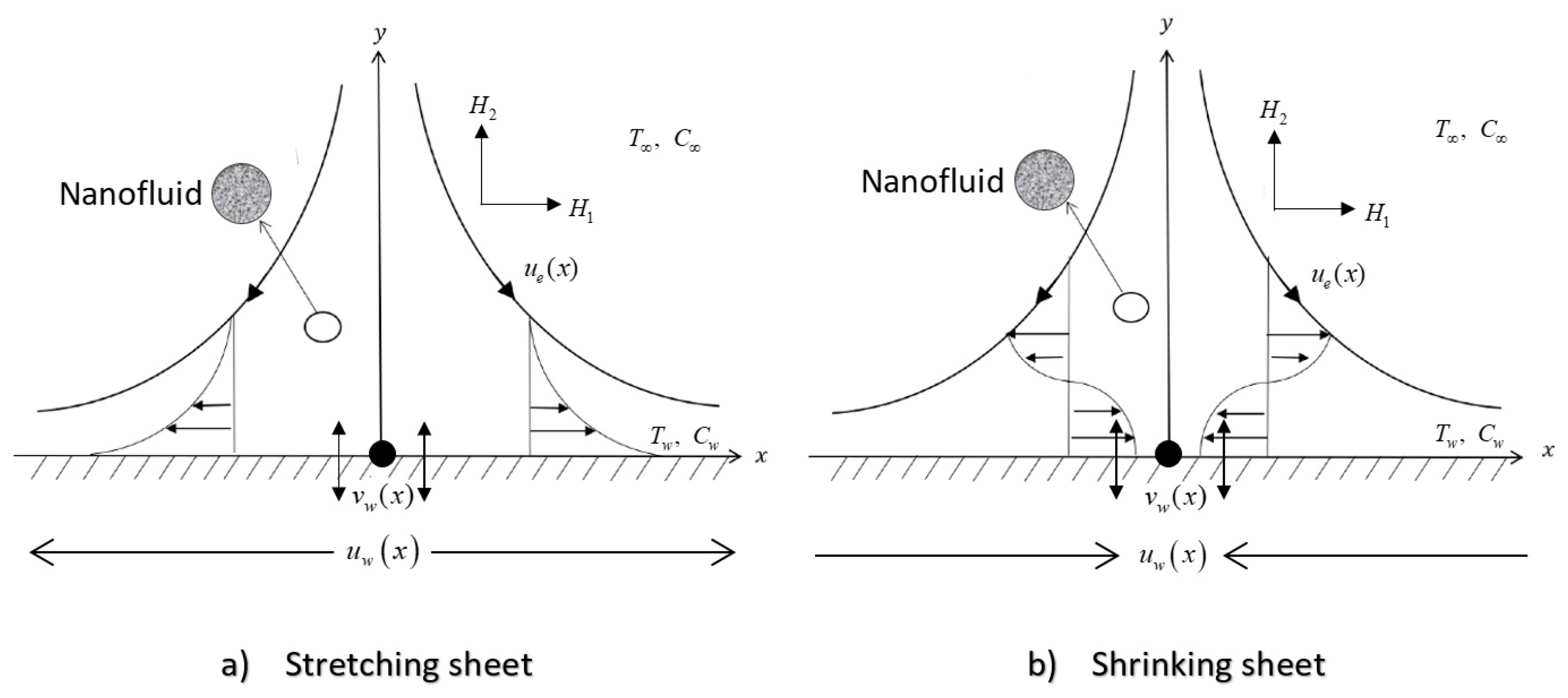
2. Problem Formulation

We consider a steady two-dimensional MHD stagnation-point flow of heat and mass transfer over a permeable stretching/shrinking sheet in a nanofluid with induced magnetic field. The coordinate system is selected, in which the x–axis is in horizontal direction and the y-axis is in vertical direction. u and v represents the velocity and $H_1$ and $H_2$ are the magnetic components along the x– and y–axes, respectively. $u_e$ is the velocity at the edge of the boundary layer while $u_w$ and $v_w$ are, respectively, the velocity and mass flux velocity at the surface. At the plate, $y=0$, and the temperature T and concentration C take constant values $T_w$ and $C_w$. The ambient values as $y\to \infty$, temperature and concentration, respectively, are $T_{\infty }$ and $C_{\infty }$. The physical flow model and coordinate system are shown in Figure 1.

Following the mathematical nanofluid model proposed by Davies [52] and Kuznetsov and Nield [53], the governing equations of this problem can be derived as follows:

$$\begin{array}{c}\hfill {\displaystyle \frac{\partial u}{\partial x}}+{\displaystyle \frac{\partial v}{\partial y}}=0,\end{array}$$

(1)

$$\begin{array}{c}\hfill {\displaystyle \frac{\partial H_1}{\partial x}}+{\displaystyle \frac{\partial H_2}{\partial y}}=0,\end{array}$$

(2)

$$\begin{array}{c}\hfill u{\displaystyle \frac{\partial u}{\partial x}}+v{\displaystyle \frac{\partial u}{\partial y}}=\nu {\displaystyle \frac{{\partial }^{2}u}{\partial y^2}}+u_e{\displaystyle \frac{d{u}_e}{dx}}+{\displaystyle \frac{\mu }{4\pi \rho }}\left(H_1{\displaystyle \frac{\partial H_1}{\partial x}}+H_2{\displaystyle \frac{\partial H_1}{\partial y}}\right)‒{\displaystyle \frac{\mu H_e}{4\pi \rho }}{\displaystyle \frac{d{H}_e}{dx}},\end{array}$$

(3)

$$u{\displaystyle \frac{\partial H_1}{\partial x}}+v{\displaystyle \frac{\partial H_1}{\partial y}}‒H_1{\displaystyle \frac{\partial u}{\partial x}}‒H_2{\displaystyle \frac{\partial u}{\partial y}}={\mu }_e{\displaystyle \frac{{\partial }^2{H}_1}{\partial y^2}},$$

(4)

$$\begin{array}{c}\hfill u{\displaystyle \frac{\partial T}{\partial x}}+v{\displaystyle \frac{\partial T}{\partial y}}=\alpha {\displaystyle \frac{{\partial }^{2}T}{\partial y^2}}+ϵ\left[D_B{\displaystyle \frac{\partial C}{\partial y}}{\displaystyle \frac{\partial T}{\partial y}}+{\displaystyle \frac{D_T}{T_{\infty }}}{\left({\displaystyle \frac{\partial T}{\partial y}}\right)}^2\right],\end{array}$$

(5)

$$\begin{array}{c}\hfill u{\displaystyle \frac{\partial C}{\partial x}}+v{\displaystyle \frac{\partial C}{\partial y}}=D_B{\displaystyle \frac{{\partial }^{2}C}{\partial y^2}}+{\displaystyle \frac{D_T}{T_{\infty }}}{\displaystyle \frac{{\partial }^{2}T}{\partial y^2}},\end{array}$$

(6)

along with their boundary conditions:

$$\begin{array}{c}\hfill u=\lambda u_w\left(x\right),v=v_w\left(x\right),{\displaystyle \frac{\partial H_1}{\partial y}}=0,H_2=0,T=T_w,D_B{\displaystyle \frac{\partial C}{\partial y}}+{\displaystyle \frac{D_T}{T_{\infty }}}{\displaystyle \frac{\partial T}{\partial y}}=0\mathrm{at}y=0,\\ \hfill u=u_e\to ax,H_1=H_e\left(x\right)\to H_0\left(x\right),T\to T_{\infty },C\to C_{\infty }\mathrm{as}y\to \infty ,\end{array}$$

(7)

where $ϵ={\displaystyle \frac{{\left(\rho C_p\right)}_p}{{\left(\rho C_p\right)}_f}}$ is defined as the ratio of nanoparticle heat capacity to the base fluid heat capacity. The boundary conditions $D_B{\displaystyle \frac{\partial C}{\partial y}}+{\displaystyle \frac{D_T}{T_{\infty }}}{\displaystyle \frac{\partial T}{\partial y}}=0$ at $y=0$ in Equation (7) states that the normal flux of nanoparticles is zero at the boundary when the thermophoresis is considered (Kuznetsov and Nield [51]).

Following Kuznetsov and Nield [53], we introduce symmetry variables

$$\begin{array}{c}\hfill \eta ={\left({\displaystyle \frac{a}{\alpha }}\right)}^{1/2}y,u=ax{f}^{{}^{\prime }}\left(\eta \right),v=‒{\left(a\alpha \right)}^{1/2}f\left(\eta \right),H_1=H_{0}x{h}^{\prime }\left(\eta \right),\\ \hfill H_2=‒{\left({\displaystyle \frac{\alpha }{a}}\right)}^{1/2}{H}_{0}h\left(\eta \right),\theta \left(\eta \right)={\displaystyle \frac{T‒T_{\infty }}{T_w‒T_{\infty }}},\varphi \left(\eta \right)={\displaystyle \frac{C‒C_{\infty }}{C_{\infty }}},\end{array}$$

(8)

where primes denote differentiation with respect to $\eta$.

After substitution Equation (8) into Equations (1)–(6), we get the following reduced form:

$$\begin{array}{c}\hfill Pr{f}^{{}^{‴}}+f{f}^{{}^{″}}‒f^{{}^{\prime 2}}+1+M(h^{{}^{\prime 2}}‒h{h}^{{}^{″}}‒1)=0,\end{array}$$

(9)

$$\chi h^{{}^{‴}}+f{h}^{{}^{″}}‒f^{{}^{″}}h=0,$$

(10)

$${\theta }^{{}^{″}}+f{\theta }^{{}^{\prime }}+Nb{\varphi }^{{}^{\prime }}{\theta }^{{}^{\prime }}+Nt{\theta }^{{}^{\prime 2}}=0,$$

(11)

$${\varphi }^{{}^{″}}+Lef{\varphi }^{{}^{\prime }}+{\displaystyle \frac{Nt}{Nb}}{\theta }^{{}^{″}}=0,$$

(12)

subjected to the new boundary conditions:

$$\begin{array}{c}\hfill f\left(0\right)=S,f^{{}^{\prime }}\left(0\right)=\lambda ,h\left(0\right)=0,h^{{}^{″}}\left(0\right)=0,\theta \left(0\right)=1,Nb{\varphi }^{{}^{\prime }}+Nt{\theta }^{{}^{\prime }}=0,\\ \hfill f^{{}^{\prime }}(\infty )\to 1,h^{{}^{\prime }}(\infty )\to 1,\theta (\infty )\to 0,\varphi (\infty )\to 0.\end{array}$$

(13)

In the above equations, $Pr$ is the Prandtl number, M is the magnetic parameter, $\chi$ is the reciprocal magnetic parameter, $Nb$ is the Brownian motion parameter, $Nt$ is the thermophoresis parameter, $Le$ is the Lewis number, S is the suction/injection parameter which is defined as

$$\begin{array}{c}\hfill Pr={\displaystyle \frac{\nu }{\alpha }},M={\displaystyle \frac{\mu H_0^2}{4\pi \rho a^2}},\chi ={\displaystyle \frac{{\mu }_e}{\nu }},Nb={\displaystyle \frac{ϵD_B{C}_w}{\alpha }},\\ \hfill Nt={\displaystyle \frac{ϵD_T(T‒T_{\infty })}{\alpha T_{\infty }}},Le={\displaystyle \frac{\alpha }{D_B}},S=‒{\displaystyle \frac{v_0}{{\left(a\alpha \right)}^{1/2}}},\end{array}$$

(14)

and $\lambda$ stands for stretching/shrinking parameter. Here, $\lambda >0$ indicates that the plate is stretched; while when $\lambda <0$ the plate is shrunk. It should be highlighted that the use of the variables (8) will change the position of the $Pr$ from the energy Equation (11) to the momentum Equation (9), which is a new fact for stretching/shrinking sheet problems.

The physical quantities of interest in this study are the skin friction or shear stress coefficient $C_f$ and the local Nusselt number $N{u}_x$ are

$$\begin{array}{c}\hfill C_f={\displaystyle \frac{{\tau }_w}{\rho u_e^2}},N{u}_x={\displaystyle \frac{x{q}_w}{k(T_w‒T_{\infty })}}.\end{array}$$

(15)

Here ${\tau }_w$ is the surface shear stress and $q_w$ is the surface heat flux given by

$$\begin{array}{c}\hfill {\tau }_w=\mu {\left({\displaystyle \frac{\partial u}{\partial y}}\right)}_{y=0},q_w=‒k{\left({\displaystyle \frac{\partial T}{\partial y}}\right)}_{y=0}.\end{array}$$

(16)

Then, applying the symmetry variables (8), we obtain

$$\begin{array}{c}\hfill C_{f}R{e}_x^{1/2}P{r}^{‒1/2}=f^{{}^{″}}\left(0\right),N{u}_{x}R{e}_x^{‒1/2}P{r}^{‒1/2}=‒{\theta }^{{}^{\prime }}\left(0\right),\end{array}$$

(17)

where $R{e}_x=u_{e}x/\nu$ is the local Reynolds number. However, the local Sherwood number $S{h}_x$ can be derived from the boundary conditions (13) as ${\varphi }^{{}^{\prime }}\left(0\right)=‒{\displaystyle \frac{Nt}{Nb}}{\theta }^{{}^{\prime }}\left(0\right)$.

3. Stability Analysis

To conduct the stability analysis of the solutions, we consider this problem in unsteady form. The continuity in Equations (1) and (2) hold, in the time Equations (3)–(6) are redressed by

$$\begin{array}{c}\hfill {\displaystyle \frac{\partial u}{\partial t}}+u{\displaystyle \frac{\partial u}{\partial x}}+v{\displaystyle \frac{\partial u}{\partial y}}=\nu {\displaystyle \frac{{\partial }^{2}u}{\partial y^2}}+u_e{\displaystyle \frac{d{u}_e}{dx}}+{\displaystyle \frac{\mu }{4\pi \rho }}\left(H_1{\displaystyle \frac{\partial H_1}{\partial x}}+H_1{\displaystyle \frac{\partial H_2}{\partial y}}\right)‒{\displaystyle \frac{\mu H_e}{4\pi \rho }}{\displaystyle \frac{d{H}_e}{dx}},\end{array}$$

(18)

$$\begin{array}{c}\hfill {\displaystyle \frac{\partial H_1}{\partial t}}+u{\displaystyle \frac{\partial H_1}{\partial x}}+v{\displaystyle \frac{\partial H_1}{\partial y}}‒H_1{\displaystyle \frac{\partial u}{\partial x}}‒H_2{\displaystyle \frac{\partial u}{\partial y}}={\mu }_e{\displaystyle \frac{{\partial }^2{H}_1}{\partial y^2}},\end{array}$$

(19)

$$\begin{array}{c}\hfill {\displaystyle \frac{\partial T}{\partial t}}+u{\displaystyle \frac{\partial T}{\partial x}}+v{\displaystyle \frac{\partial T}{\partial y}}=\alpha {\displaystyle \frac{{\partial }^{2}T}{\partial y^2}}+ϵ\left[D_B{\displaystyle \frac{\partial C}{\partial y}}{\displaystyle \frac{\partial T}{\partial y}}+{\displaystyle \frac{D_T}{T_{\infty }}}{\left({\displaystyle \frac{\partial T}{\partial y}}\right)}^2\right],\end{array}$$

(20)

$$\begin{array}{c}\hfill {\displaystyle \frac{\partial C}{\partial t}}+u{\displaystyle \frac{\partial C}{\partial x}}+v{\displaystyle \frac{\partial C}{\partial y}}=D_B{\displaystyle \frac{{\partial }^{2}C}{\partial y^2}}+{\displaystyle \frac{D_T}{T_{\infty }}}{\displaystyle \frac{{\partial }^{2}T}{\partial y^2}},\end{array}$$

(21)

where t denotes the time. The following new dimensionless variables are introduced:

$$\begin{array}{c}\hfill \eta ={\left({\displaystyle \frac{a}{\alpha }}\right)}^{1/2}y,\tau =at,u=ax{f}^{{}^{\prime }}(\eta ,\tau ),v=‒{\left(a\alpha \right)}^{1/2}f(\eta ,\tau ),H_1=H_{0}x{h}^{\prime }(\eta ,\tau ),\\ \hfill H_2=‒{\left({\displaystyle \frac{\alpha }{a}}\right)}^{1/2}{H}_{0}h(\eta ,\tau ),\theta (\eta ,\tau )={\displaystyle \frac{T‒T_{\infty }}{T_w‒T_{\infty }}},\varphi (\eta ,\tau )={\displaystyle \frac{C‒C_{\infty }}{C_{\infty }}},\end{array}$$

(22)

thus, Equations (18)–(21) can be composed as

$$\begin{array}{c}\hfill Pr{\displaystyle \frac{{\partial }^{3}f}{\partial {\eta }^3}}‒{\left({\displaystyle \frac{\partial f}{\partial \eta }}\right)}^2+f{\displaystyle \frac{{\partial }^{2}f}{\partial {\eta }^2}}+1+M\left[{\left({\displaystyle \frac{\partial h}{\partial \eta }}\right)}^2‒h\left({\displaystyle \frac{{\partial }^{2}h}{\partial {\eta }^2}}\right)‒1\right]‒{\displaystyle \frac{{\partial }^{2}f}{\partial \eta \partial \tau }}=0,\end{array}$$

(23)

$$\begin{array}{c}\hfill \chi {\displaystyle \frac{{\partial }^{3}h}{\partial {\eta }^3}}+f{\displaystyle \frac{{\partial }^{2}h}{\partial {\eta }^2}}‒h{\displaystyle \frac{{\partial }^{2}f}{\partial {\eta }^2}}‒{\displaystyle \frac{{\partial }^{2}h}{\partial \eta \partial \tau }}=0,\end{array}$$

(24)

$$\begin{array}{c}\hfill {\displaystyle \frac{{\partial }^2\theta }{\partial {\eta }^2}}+f{\displaystyle \frac{\partial \theta }{\partial \eta }}+Nb{\displaystyle \frac{\partial \varphi }{\partial \eta }}{\displaystyle \frac{\partial \theta }{\partial \eta }}+Nt{\left({\displaystyle \frac{\partial \theta }{\partial \eta }}\right)}^2‒{\displaystyle \frac{\partial \theta }{\partial \tau }}=0,\end{array}$$

(25)

$$\begin{array}{c}\hfill {\displaystyle \frac{{\partial }^2\varphi }{\partial {\eta }^2}}+Lef{\displaystyle \frac{\partial \theta }{\partial \eta }}+{\displaystyle \frac{Nt}{Nb}}{\displaystyle \frac{{\partial }^2\varphi }{\partial {\eta }^2}}‒{\displaystyle \frac{\partial \varphi }{\partial \tau }}=0,\end{array}$$

(26)

along with the boundary conditions:

$$\begin{array}{c}\hfill f(0,\tau )=S,{\displaystyle \frac{\partial f}{\partial \eta }}(0,\tau )=\lambda ,h(0,\tau )=0,{\displaystyle \frac{{\partial }^{2}h}{\partial {\eta }^2}}(0,\tau )=0,\theta (0,\tau )=1,\\ \hfill Nb{\displaystyle \frac{\partial \varphi }{\partial \eta }}(0,\tau )+Nt{\displaystyle \frac{\partial \theta }{\partial \eta }}(0,\tau )=0,\\ \hfill {\displaystyle \frac{\partial f}{\partial \eta }}(\eta ,\tau )\to 1,{\displaystyle \frac{\partial h}{\partial \eta }}(\eta ,\tau )\to 0,\theta (\eta ,\tau )\to 0,\varphi (\eta ,\tau )\to 0\mathrm{as}\eta \to \infty .\end{array}$$

(27)

To check the stability of the solution $f\left(\eta \right)=f_0\left(\eta \right)$, $h\left(\eta \right)=h_0\left(\eta \right)$, $\theta \left(\eta \right)={\theta }_0\left(\eta \right)$, and $\varphi \left(\eta \right)={\varphi }_0\left(\eta \right)$ attaining the boundary value problem (9)–(12), we write

$$\begin{array}{c}\hfill f(\eta ,\tau )=f_0\left(\eta \right)+e^{‒\gamma \tau }F(\eta ,\tau ),h(\eta ,\tau )=h_0\left(\eta \right)+e^{‒\gamma \tau }H(\eta ,\tau ),\\ \hfill \theta (\eta ,\tau )={\theta }_0\left(\eta \right)+e^{‒\gamma \tau }T(\eta ,\tau ),\varphi (\eta ,\tau )={\varphi }_0\left(\eta \right)+e^{‒\gamma \tau }P(\eta ,\tau ),\end{array}$$

(28)

where $F(\eta ,\tau )$, $H(\eta ,\tau )$, $T(\eta ,\tau )$, and $P(\eta ,\tau )$ are small relative to $f_0\left(\eta \right)$, $h_0\left(\eta \right)$, ${\theta }_0\left(\eta \right)$, ${\varphi }_0\left(\eta \right)$, respectively, and $\gamma$ is an unknown eigenvalue. Introducing (28) into Equations (23)–(27), we get the following linearized problem:

$$\begin{array}{c}\hfill Pr{\displaystyle \frac{{\partial }^{3}F}{\partial {\eta }^3}}+f_0{\displaystyle \frac{{\partial }^{2}F}{\partial {\eta }^2}}‒\left(2f_0^{{}^{\prime }}‒\gamma \right){\displaystyle \frac{\partial F}{\partial \eta }}+f_0^{{}^{″}}F+M\left[2h_0^{{}^{\prime }}{\displaystyle \frac{\partial H}{\partial \eta }}‒h_0{\displaystyle \frac{{\partial }^{2}H}{\partial {\eta }^2}}‒h_0^{{}^{″}}H\right]‒{\displaystyle \frac{{\partial }^{2}F}{\partial \eta \partial \tau }}=0,\end{array}$$

(29)

$$\begin{array}{c}\hfill \chi {\displaystyle \frac{{\partial }^{3}H}{\partial {\eta }^3}}+f_0{\displaystyle \frac{{\partial }^{2}H}{\partial {\eta }^2}}‒h_0{\displaystyle \frac{{\partial }^{2}F}{\partial {\eta }^2}}+h_0^{{}^{″}}F‒f_0^{{}^{″}}H+\gamma {\displaystyle \frac{\partial H}{\partial \eta }}‒{\displaystyle \frac{{\partial }^{2}H}{\partial \eta \partial \tau }}=0,\end{array}$$

(30)

$$\begin{array}{c}\hfill {\displaystyle \frac{{\partial }^{2}T}{\partial {\eta }^2}}+f_0{\displaystyle \frac{\partial T}{\partial \eta }}+{\theta }_0^{{}^{\prime }}F+Nt\left(2{\theta }_0^{{}^{\prime }}{\displaystyle \frac{\partial T}{\partial \eta }}\right)+Nb\left({\varphi }_0^{{}^{\prime }}{\displaystyle \frac{\partial T}{\partial \eta }}+{\theta }_0^{{}^{\prime }}{\displaystyle \frac{\partial P}{\partial \eta }}\right)+\gamma T‒{\displaystyle \frac{\partial T}{\partial \tau }}=0,\end{array}$$

(31)

$$\begin{array}{c}\hfill {\displaystyle \frac{{\partial }^{2}P}{\partial {\eta }^2}}+Le\left(f_0{\displaystyle \frac{\partial P}{\partial \eta }}+{\varphi }_0^{{}^{\prime }}F\right)+{\displaystyle \frac{Nt}{Nb}}{\displaystyle \frac{{\partial }^{2}T}{\partial {\eta }^2}}+\gamma P‒{\displaystyle \frac{\partial P}{\partial \tau }}=0,\end{array}$$

(32)

the boundary conditions in Equation (27) are now reduced to

$$\begin{array}{c}\hfill F(0,\tau )=0,{\displaystyle \frac{\partial F}{\partial \eta }}(0,\tau )=0,H(0,\tau )=0,{\displaystyle \frac{{\partial }^{2}H}{\partial {\eta }^2}}(0,\tau )=0,T(0,\tau )=0,\\ \hfill Nb{\displaystyle \frac{\partial P}{\partial \eta }}(0,\tau )+Nt{\displaystyle \frac{\partial T}{\partial \eta }}(0,\tau )=0,\\ \hfill {\displaystyle \frac{\partial F}{\partial \eta }}(\eta ,\tau )\to 0,H(\eta ,\tau )\to 0,T(\eta ,\tau )\to 0,P(\eta ,\tau )\to 0\mathrm{as}\eta \to \infty .\end{array}$$

(33)

The solutions $f\left(\eta \right)=f_0\left(\eta \right)$, $h\left(\eta \right)=h_0\left(\eta \right)$, and $\theta \left(\eta \right)={\theta }_0\left(\eta \right)$ of the steady flow Equations (9)–(13) are obtained by setting $\tau =0$. Accordingly, $F\left(\eta \right)=F_0\left(\eta \right)$, $H\left(\eta \right)=H_0\left(\eta \right)$, and $T\left(\eta \right)=T_0\left(\eta \right)$ in Equations (29)–(32) pinpoint the initial growth or decay of perturbation of the solution (28). In this regard, we need to work out the following linear eigenvalue problem:

$$\begin{array}{c}\hfill Pr{F}_0^{{}^{‴}}+f_0^{{}^{″}}{F}_0+f_0{F}_0^{{}^{″}}‒\left(2f_0^{{}^{\prime }}‒\gamma \right)F_0^{{}^{\prime }}+M\left(2h_0^{{}^{\prime }}{H}_0^{{}^{\prime }}‒h_0{H}_0^{{}^{″}}‒h_0^{{}^{″}}H\right)=0,\end{array}$$

(34)

$$\begin{array}{c}\hfill \chi H_0^{{}^{‴}}+f_0{H}_0^{{}^{″}}+h_0^{{}^{″}}{F}_0‒f_0^{{}^{″}}{H}_0‒h_0{F}_0^{{}^{″}}+\gamma H_0^{{}^{\prime }}=0,\end{array}$$

(35)

$$\begin{array}{c}\hfill T_0^{{}^{″}}+f_0{T}_0^{{}^{\prime }}+{\theta }_0^{{}^{\prime }}{F}_0+Nt\left(2{\theta }_0^{{}^{\prime }}{T}_0^{{}^{\prime }}\right)+Nb\left({\varphi }_0^{{}^{\prime }}{T}_0^{{}^{\prime }}+{\theta }_0^{{}^{\prime }}{P}_0^{{}^{\prime }}\right)+\gamma T_0=0,\end{array}$$

(36)

$$\begin{array}{c}\hfill P_0^{{}^{″}}+Le\left(f_0{T}_0^{{}^{\prime }}+{\varphi }_0^{{}^{\prime }}{F}_0\right)+{\displaystyle \frac{Nt}{Nb}}{T}_0^{{}^{″}}+\gamma P_0=0,\end{array}$$

(37)

along with the boundary conditions:

$$\begin{array}{c}\hfill F_0\left(0\right)=0,F_0^{{}^{\prime }}\left(0\right)=0,H_0\left(0\right)=0,H_0^{{}^{″}}\left(0\right)=0,T_0\left(0\right)=0,Nb{P}_0^{{}^{\prime }}\left(0\right)+Nt{T}_0^{{}^{\prime }}\left(0\right)=0,\\ \hfill F_0^{{}^{\prime }}\left(\eta \right)\to 0,H_0^{{}^{\prime }}\left(\eta \right)\to 0,T_0\left(\eta \right)\to 0,P_0\left(\eta \right)\to 0\mathrm{as}\eta \to \infty .\end{array}$$

(38)

The smallest eigenvalue ${\gamma }_1$ obtained delineates the stability of this dual solution of the steady-state flow. Consequently, as recommended by Harris et al. [54], the boundary condition $F_0^{{}^{\prime }}\left(\eta \right),H_0^{{}^{\prime }}\left(\eta \right),T_0\left(\eta \right)$, and $P_0\left(\eta \right)$ can be put at rest in order to demonstrate the range of possible eigenvalue. In this problem, the condition $F_0^{{}^{\prime }}\left(\eta \right)$ as $\eta \to \infty$ is chosen to be relaxed and, for a fixed value of $\gamma$, the following system of Equations (34)–(38) will be solved by introducing a new boundary condition which is $F_0^{{}^{″}}\left(0\right)=1$.

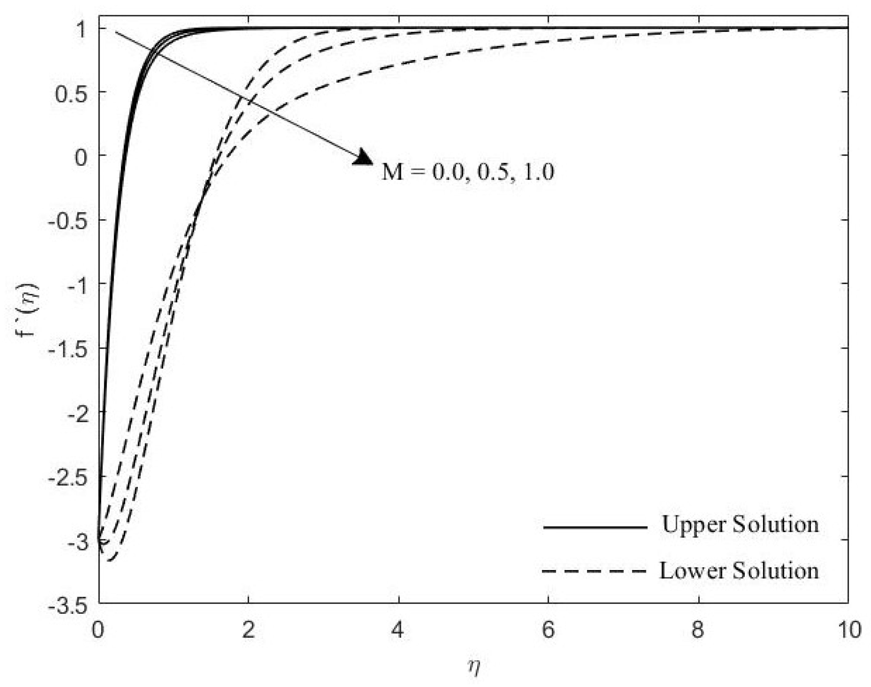
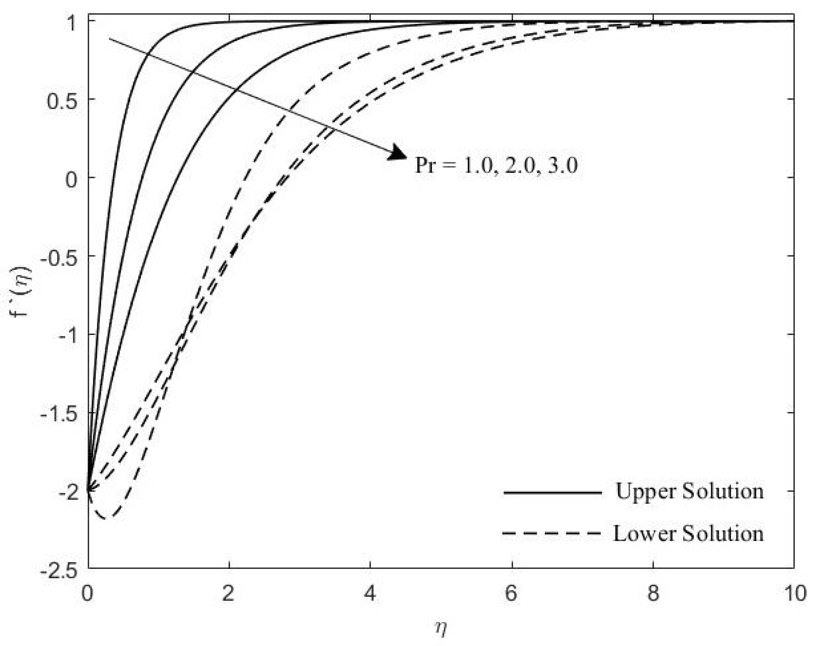
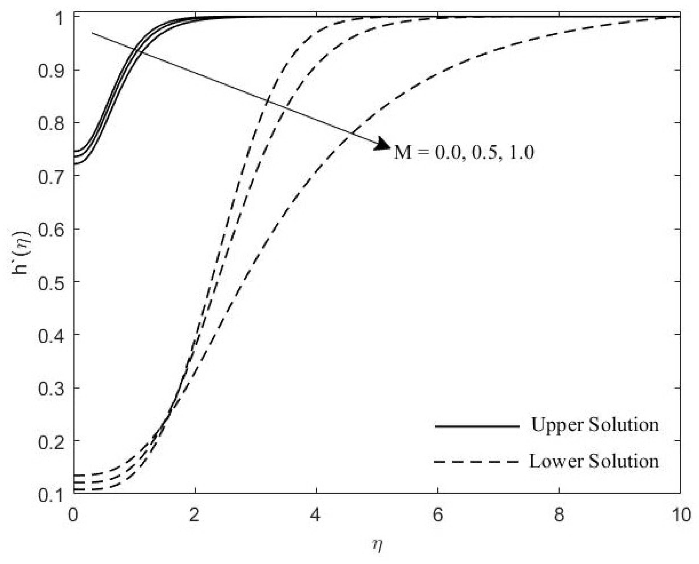
4. Results and Discussion

The governing Equations (9)–(12) together with the boundary conditions (13) have been numerically-solved adopting bvp4c function in Matlab solver. It should be emphasized that the parameters used in this study are the $Pr$(0.72–3), M(0.0–0.5), $\chi$(1–3), $Le$(1–5), $Nb$(0.01–0.05), $Nt$(0.01–0.05), S(0–3), and $\lambda (\le 2)$. We fix $Pr=0.72$, $M=0.5$, $\chi =1$, $Le=1$, $Nb=0.01$, $Nt=0.01$, and $S=3$ into our computation procedure, modifying one parameter at a time. We take ${\eta }_{\infty }=10$ as our far-field boundary condition. All the profiles presented in the form of figures (Figure 2, Figure 3, Figure 4, Figure 5, Figure 6, Figure 7, Figure 8, Figure 9 and Figure 10) satisfy the boundary condition (13) and produce asymptotic graph. A comparison of the results for some values of $f^{″}\left(0\right)$ has been carried out with the results in the existing literature [55,56] in order to validate this study. This comparison data is shown in

Table 1. Comparison values of the skin friction coefficient $f^{″}\left(0\right)$ for some values of $\lambda$ when $M=0$.

$\mathit{\lambda }$	Present Result		Aman et al. [55]		Bhattacharyya et al. [56]
	Upper Branch	Lower Branch	Upper Branch	Lower Branch	Upper Branch	Lower Branch
−0.25	1.40224		1.4022		1.40224051
−0.3	1.42758		1.4276
−0.4	1.46861		1.4686
−0.5	1.49567		1.4957		1.49566948
−0.615	1.50724		1.5072		1.50724089
−0.75	1.48929		1.4893		1.48929834
−1.0	1.32881	0	1.3288	0	1.32881689	0
−1.15	1.08223	0.11670	1.0822	0.1167	1.08223164	0.11667340
−1.18	1.00045	0.17836	1.0004	0.1784
−1.2465	0.55430	0.55430	0.5543	0.5543	0.55428565	0.55428565

and shows a positive agreement. Consequently, we are assured that the numerical values obtained in this study are veritable.

Figure 2 and Figure 3 show the velocity profiles with the effects of M and $Pr$, respectively. It is seen that as the value of M and $Pr$ increases, the boundary layer thickness of these profiles also increase. Figure 4, Figure 5 and Figure 6 portray the impact of M, $\chi$, and $Pr$ on the induced magnetic profiles. As the value of these parameters increase, the boundary layer thickness become thicker. Figure 7 illustrates the influence of the $Pr$ on temperature profile. It is noticed that the thermal boundary layer thickness increases as the $Pr$ increase.

Figure 8, Figure 9 and Figure 10 demonstrate the concentration profile with respect to the changes of $Le$, $Nt$, and $Nb$, respectively. Figure 8 exhibits the influence of $Le$ on concentration graph profile. The concentration boundary layer thickness decreases as Lewis number increases. This is likely due to the fact that mass transfer rate increases parallel to $Le$. Likewise divulges that the concentration gradient at the plate surface is also increasing. As can be seen in Figure 9, increasing values of $Nt$ leads to an increase in the thickness of concentration graph profile. A different behavior is shown in Figure 10, the concentration graph profile is decreasing when the value of $Nb$ increasing. Thus, the concentration boundary layer also decreases. From these figures it may very well be seen that the boundary layer thickness for the upper solution is slightly slimmer contrasted with that of the lower branch solution.

Figure 11, Figure 12, Figure 13 and Figure 14 illustrate the dual solutions for the skin friction coefficient $f^{″}\left(0\right)$ and the local Nusselt number $‒{\theta }^{\prime }\left(0\right)$. Based on the observation, dual solutions of Equations (9)–(12) can be obtained both for shrinking $(\lambda <0)$ and stretching $(\lambda >0)$ cases. Figure 11 exhibits the variation of the $f^{″}\left(0\right)$ increasing as the value of S increases. The presence of suction will escalate the skin friction at the surface of sheet. Thereupon, the flow speed will decrease and as a result increase the velocity gradient at the surface of the sheet. The variation of the $‒{\theta }^{\prime }\left(0\right)$, as shown in Figure 12, indicates that when S increases, the heat transfer rate at the surface also increases. The heat flux becomes larger when suction is applied in the flow. Hence, it will also increase the magnitude of the temperature gradient at the surface of the sheet. Based on the critical value ${\lambda }_c$ in these figures, the influence of suction S also causes a delaying of the boundary layer separation. From Figure 13 and Figure 14, we can observe that as the values of M increase, the $f^{″}\left(0\right)$ and $‒{\theta }^{\prime }\left(0\right)$ decrease. In magnetohydrodynamics problems, it is a fact that the presence of transverse magnetic field sets in Lorentz force, which exudes a retarding force on the velocity field. The existing of this force has the urgency to decelerate the fluid motion in the boundary layer. As a result, the boundary layer separation occurs faster when the magnetic field is adapted.

Based on all these figures, the existence of nonunique solutions (dual solutions) are clearly shown. The stability of these solutions are tested to analyze which solutions are stable and physically realizable in practice. It is also intended to find out which solutions are not suitable as well. Therefore, the eigenvalue problem (34)–(38) is solved for the smallest eigenvalues ${\gamma }_1$ regarding the upper and lower solution branches. These calculations are presented in

Table 2. Smallest eigenvalue ${\gamma }_1$ for some values of $\lambda$ with different S.

S	$\mathit{\lambda }$	First Solution	Second Solution
1	−1.8	0.40484	−0.39610
	−1.82	0.12550	−0.12458
	−1.822	0.03052	−0.03049
2	−2.8	0.73421	−0.71159
	−2.85	0.28333	−0.27970
	−2.858	0.08134	−0.08104
3	−4.3	0.42854	−0.42058
	−4.31	0.25712	−0.25423
	−4.315	0.08807	−0.08773

for some values of $\lambda$ when $S=1,2,3$. From the table, it can be noticed that the smallest eigenvalue ${\gamma }_1$ gives a positive value for the first solution and a negative value for the second solution. Hence, a conclusion is drawn that only the upper branch solutions are physically significant; whilst the lower branch solutions are not. Furthermore, as the value of $\lambda$ approaches the critical point ${\lambda }_c$, the smallest eigenvalue ${\gamma }_1$ converges to 0 for both upper and lower branches, as discovered by Merkin [49].

5. Conclusions

A numerical study is carried out for the revised model of the steady MHD stagnation-point flow of nanofluid over a stretching or shrinking sheet with induced magnetic field. The effect of all parameters are studied numerically and graphically. The suction detains the boundary layer separation, however, the magnetic parameter enhances the boundary layer separation. Non-unique (dual) solutions are found to exist for both stretching and shrinking cases. Therefore, a stability analysis is done via bvp4c function in MATLAB software, and their results found that the first solution (upper branch) is stable and valid physically; while the second solution (lower branch) is not stable.

References

1. Fisher, E.G. Extrusion of Plastics, 3rd ed.; Wiley: New York, NY, USA, 1976. [Google Scholar]
2. Tsou, F.K.; Sparrow, E.M.; Goldstein, R.J. Flow and heat transfer in the boundary layer on a continuous moving surface. Int. J. Heat Mass Transf. 1967, 10, 219–235. [Google Scholar] [CrossRef]
3. Sakiadis, B.C. Boundary-layer behavior on continuous solid surfaces: I. Boundary-layer equations for two-dimensional and axisymmetric flow. AIChE J. 1961, 7, 26–28. [Google Scholar] [CrossRef]
4. Crane, L.J. Flow past a stretching plate. J. Appl. Math. Phys. (ZAMP) 1970, 21, 645–647. [Google Scholar] [CrossRef]
5. Miklavčič, M.; Wang, C.Y. Viscous flow due to a shrinking sheet. Q. Appl. Math. 2006, 64, 283–290. [Google Scholar] [CrossRef] [Green Version]
6. Wang, C.Y. Stagnation flow towards a shrinking sheet. Int. J. Non-Linear Mech. 2008, 43, 377–382. [Google Scholar] [CrossRef]
7. Shercliff, J.A. A Textbook of Magnetohydrodynamics; Pergamon Press: Oxford, UK; New York, NY, USA, 1965. [Google Scholar]
8. Branover, G.G.; Tinober, A.B. Magnetohydrodynamics of Incompressible Media (in Russian); Nauka: Moscow, Russia, 1970. [Google Scholar]
9. Cramer, K.R.; Pai, S.I. Magneto Fluid Dynamics For Engineers and Applied Physicists; McGraw-Hill Book Company: Washington, DC, USA, 1973. [Google Scholar]
10. Apelblat, A. Application of the Laplace transform to the solution of the boundary layer equations. III: Magnetohydrodynamic Falkner-Skan problem. J. Phys. Soc. Jpn. 1969, 27, 235–239. [Google Scholar] [CrossRef]
11. Ingham, D.B. Impulsively started viscous flows past a finite flat plate with and without an applied magnetic field. Int. J. Numer. Methods Eng. 1973, 6, 521–527. [Google Scholar] [CrossRef]
12. Liron, N.; Wilhelm, H.E. Integration of the Magnetohydrodynamic boundary-layer equations by Meksyn’s method. J. Appl. Math. Mech. (ZAMM) 1974, 54, 27–37. [Google Scholar] [CrossRef]
13. Watanabe, T.; Pop, I. Magnetohydrodynamic free convection flow over a wedge in the presence of a transverse magnetic field. Int. Commun. Heat Mass Trans. 1993, 20, 871–881. [Google Scholar] [CrossRef]
14. Gul, A.; Khan, I.; Shafie, S.; Khalid, A.; Khan, A. Heat transfer in MHD mixed convection flow of a ferrofluid along a vertical channel. PLoS ONE 2015, 10, e0141213. [Google Scholar] [CrossRef]
15. Kishore, P.M.; Rajesh, V.; Verma, V. Effects of heat transfer and viscous dissipation on MHD free convection flow past an exponentially accelerated vertical plate with variable temperature. J. Nav. Archit. Mar. Eng. 2010, 7, 101–110. [Google Scholar] [CrossRef]
16. Shehzad, S.A.; Abdullah, Z.; Alsaedi, A.; Abbasi, F.M.; Hayat, T. Thermally radiative three-dimensional flow of Jeffrey nanofluid with internal heat generation and magnetic field. J. Magn. Magn. Mater. 2016, 397, 108–114. [Google Scholar] [CrossRef]
17. Hayat, T.; Waqas, M.; Khan, M.I.; Alsaedi, A. Impacts of constructive and destructive chemical reactions in magnetohydrodynamic (MHD) flow of Jeffrey liquid due to nonlinear radially stretched surface. J. Mol. Liq. 2017, 225, 302–310. [Google Scholar] [CrossRef]
18. Tashtoush, B.; Magableh, A. Magnetic field effect on heat transfer and fluid flow characteristics of blood flow in multi-stenosis arteries. Heat Mass Trans. 2008, 44, 297–304. [Google Scholar] [CrossRef]
19. Mukhopadhyay, S. MHD boundary layer flow and heat transfer over an exponentially stretching sheet embedded in a thermally stratified medium. Alexendria Eng. J. 2013, 52, 259–265. [Google Scholar] [CrossRef] [Green Version]
20. Tian, X.; Li, B.; Zhang, J. The effects of radiation optical properties on the unsteady 2D boundary layer MHD flow and heat transfer over a stretching plate. Int. J. Heat Mass Transf. 2017, 105, 109–112. [Google Scholar] [CrossRef]
21. Ali, F.M.; Nazar, R.; Arifin, N.M.; Pop, I. Dual solutions in MHD flow on a nonlinear porous shrinking sheet in a viscous fluid. Bound. Value Probl. 2013, 1, 32. [Google Scholar] [CrossRef]
22. Jusoh, R.; Nazar, R.; Pop, I. Magnetohydrodynamic rotating flow and heat transfer of ferrofluid due to an exponentially permeable stretching/shrinking sheet. J. Magn. Magn. Mater. 2018, 465, 365–374. [Google Scholar] [CrossRef]
23. Ali, F.M.; Nazar, R.; Arifin, N.M.; Pop, I. MHD mixed convection boundary layer flow toward a stagnation point on a vertical surface with induced magnetic field. ASME J. Heat Transf. 2011, 133, 022502. [Google Scholar] [CrossRef]
24. Ali, F.M.; Nazar, R.; Arifin, N.M.; Pop, I. MHD boundary layer flow and heat transfer over a stretching sheet with induced magnetic field. Heat Mass Trans. 2011, 47, 155–162. [Google Scholar] [CrossRef]
25. Choi, S.U.S.; Eastman, J.A. Enhancing thermal conductivity of fluids with nanoparticles. In Proceedings of the 1995 International Mechanical Engineering Congress and Exposition, San Francisco, CA, USA, 12–17 November 1995; Volume 66, pp. 99–105. [Google Scholar]
26. Xie, H.; Wang, J.; Xi, T.; Liu, Y.; Ai, F.; Wu, Q. Thermal conductivity enhancement of suspensions containing nanosized alumina particles. J. Appl. Phys. 2002, 91, 4568–4572. [Google Scholar] [CrossRef]
27. Das, S.; Putra, N.; Thiesen, P.; Roetzel, W. Temperature dependence of thermal conductive enhancement for nanofluids. J. Heat Transf. 2003, 125, 567–574. [Google Scholar] [CrossRef]
28. Lee, D.; Kim, J.; Kim, B. A new parameter to control heat transport in nanofluide: Surface charge state of the particle in suspension. J. Phys. Chem. B 2006, 110, 4323–4328. [Google Scholar] [CrossRef] [PubMed]
29. Lee, J.; Hwang, K.; Jang, S.; Lee, B.; Kim, J.; Choi, S.; Choi, C. Effective viscosities and thermal conductivities of aqueous nanofluids containing low volume concentrations of Al2O3 nanoparticles. Int. J. Heat Mass Transf. 2008, 51, 2651–2656. [Google Scholar] [CrossRef]
30. Minsta, H.; Roy, G.; Nguyen, C.; Doucet, D. New temperature dependent thermal conductivity data for water based nanofluids. Int. J. Heat Mass Transf. 2009, 48, 363–371. [Google Scholar]
31. Bondareva, N.S.; Sheremet, M.A.; Oztop, H.F.; Abu-Hamdeh, N. Heatline visualization of natural convection in a thick walled open cavity filled with a nanofluid. Int. J. Heat Mass Transf. 2017, 109, 175–186. [Google Scholar] [CrossRef]
32. Saidur, R.; Leong, K.Y.; Mohammad, H.A. A review on applications and challenges of nanofluids. Renew. Sustain. Energy Rev. 2011, 15, 1646–1668. [Google Scholar] [CrossRef]
33. Das, S.K.; Choi, S.U.S.; Yu, W.; Pradeep, Y. Nanofluids: Science and Technology; Wiley: Hoboken, NJ, USA, 2008. [Google Scholar]
34. Nield, D.A.; Bejan, A. Convection in Porous Media, 4th ed.; Springer: New York, NY, USA, 2013. [Google Scholar]
35. Minkowycz, W.J.; Sparrow, E.M.; Abraham, J.P. Nanoparticle Heat Transfer and Fluid Flow; CRC Press, Taylor and Francis Group: New York, NY, USA, 2013. [Google Scholar]
36. Shenoy, A.; Sheremet, M.; Pop, I. Convective Flow and Heat Transfer from Wavy Surfaces: Viscous Fluids, Porous Media and Nanofluids; CRC Press, Taylor and Francis Group: New York, NY, USA, 2016. [Google Scholar]
37. Buongiorno, J.; Venerus, D.C.; Prabhat, N.; McKrell, T.; Townsend, J.; Christianson, R.; Tolmachev, Y.V.; Keblinski, P.; Hu, L.; Alvarado, J.L.; et al. A benchmark study on the thermal conductivity of nanofluids. J. Appl. Phys. 2009, 106, 094312. [Google Scholar] [CrossRef] [Green Version]
38. Kakaç, S.; Pramuanjaroenkij, A. Review of convective heat transfer enhancement with nanofluids. Int. J. Heat Mass Transf. 2009, 52, 3187–3196. [Google Scholar] [CrossRef]
39. Manca, O.; Jaluria, Y.; Poulikakos, D. Heat transfer in nanofluids. Adv. Mech. Eng. 2010, 2, 380826. [Google Scholar] [CrossRef]
40. Fan, J.; Wang, L. Review of heat conduction in nanofluids. ASME J. Heat Transf. 2011, 133, 040801. [Google Scholar] [CrossRef]
41. Mahian, O.; Kianifar, A.; Kalogirou, S.A.; Pop, I.; Wongwises, S. A review of the applications of nanofluids in solar energy. Int. J. Heat Mass Transf. 2013, 57, 582–594. [Google Scholar] [CrossRef]
42. Sheikholeslami, M.; Ganji, D.D. Nanofluid convective heat transfer using semi analytical and numerical approaches: A review. J. Taiwan Inst. Chem. Eng. 2016, 65, 43–77. [Google Scholar] [CrossRef]
43. Myers, T.G.; Ribera, H.; Cregan, V. Does mathematics contribute to the nanofluid debate? Int. J. Heat Mass Transf. 2017, 111, 279–288. [Google Scholar] [CrossRef] [Green Version]
44. Sheikholeslami, M.; Mehryan, S.A.M.; Shafee, A.; Sheremet, M.A. Variable magnetic forces impact on magnetizable hybrid nanofluid heat transfer through a circular cavity. J. Mol. Liq. 2019, 277, 388–396. [Google Scholar] [CrossRef]
45. Mahapatra, T.R.; Nandy, S.K. Stability of dual solutions in stagnation-point flow and heat transfer over a porous shrinking sheet with thermal radiation. Meccanica 2013, 48, 23–32. [Google Scholar] [CrossRef]
46. Hussaini, M.Y.; Lakin, W.D. Existence and non-uniqueness of similarity solutions of a boundary-layer problem. Quart. J. Mech. Appl. Math. 1986, 39, 15–24. [Google Scholar] [CrossRef]
47. Magyari, E.; Ali, M.E.; Keller, B. Heat and mass transfer characteristics of the self-similar boundary-layer flows induced by continous surfaces stretched with rapidly decreasing velocities. Heat Mass Transf. 2001, 38, 65–75. [Google Scholar] [CrossRef]
48. Merrill, K.; Beauchesne, M.; Previte, J.; Paullet, J.; Weidman, P. Final steady flow near a stagnation-point on a vertical surface in a porous medium. Int. J. Heat Mass Transf. 2006, 49, 4681–4686. [Google Scholar] [CrossRef]
49. Merkin, J.H. On dual solutions occuring in mixed convection in a porous medium. J. Eng. Math. 1985, 20, 171–179. [Google Scholar] [CrossRef]
50. Junoh, M.M.; Ali, F.M.; Pop, I. MHD stagnation-point flow of a nanofluid past a stretching/shrinking sheet with induced magnetic field. J. Eng. Appl. Sci. 2018, 13, 10474–10481. [Google Scholar]
51. Kuznetsov, A.V.; Nield, D.A. The Cheng–Minkowycz problem for natural convective boundary layer flow in a porous medium saturated by a nanofluid: A revised model. Int. J. Heat Mass Transf. 2013, 65, 682–685. [Google Scholar] [CrossRef]
52. Davies, T.V. The magneto-hydrodynamic boundary layer in two-dimensional steady flow past a semi-infinite flat plate I. Uniform conditions at infinity. Proc. R. Soc. A 1962, 273, 496–508. [Google Scholar]
53. Kuznetsov, A.V.; Nield, D.A. Natural convective boundary-layer flow of a nanofluid past a vertical plate. Int. J. Therm. Sci. 2010, 49, 243–247. [Google Scholar] [CrossRef]
54. Harris, S.D.; Ingham, D.B.; Pop, I. Mixed convection boundary-layer flow near the stagnation point on a vertical surface in a porous medium: Brinkman model with slip. Transp. Porous Media 2009, 77, 267–285. [Google Scholar] [CrossRef]
55. Aman, F.; Ishak, A.; Pop, I. Magnetohydrodynamic stagnation-point flow towards a stretching/shrinking sheet with slip effects. Int. Commun. Heat Mass Transf. 2013, 47, 68–72. [Google Scholar] [CrossRef] [Green Version]
56. Bhattacharyya, K.; Mukhopadhyay, S.; Layek, G.C. Slip effects on boundary layer stagnation-point flow and heat transfer towards a shrinking sheet. Int. J. Heat Mass Transf. 2011, 54, 308–313. [Google Scholar] [CrossRef]
Figure 1. A sketch of physical model and coordinate system.
Symmetry 11 01078 g001
Figure 2. Velocity profile for various values of M.
Symmetry 11 01078 g002
Figure 3. Velocity profile for various values of P r .
Symmetry 11 01078 g003
Figure 4. Induced magnetic profile for various values of M.
Symmetry 11 01078 g004
Figure 5. Induced magnetic profile for various values of χ .
Symmetry 11 01078 g005
Figure 6. Induced magnetic profile for various values of P r .
Symmetry 11 01078 g006
Figure 7. Temperature profile for various values of P r .
Symmetry 11 01078 g007
Figure 8. Concentration profile for various values of L e .
Symmetry 11 01078 g008
Figure 9. Concentration profile for various values of N t .
Symmetry 11 01078 g009
Figure 10. Concentration profile for various values of N b .
Symmetry 11 01078 g010
Figure 11. Variation of skin friction for various values of S.
Symmetry 11 01078 g011
Figure 12. Variation of local Nusselt number for various values of S.
Symmetry 11 01078 g012
Figure 13. Variation of skin friction for various values of M.
Symmetry 11 01078 g013
Figure 14. Variation of local Nusselt number for various values of M.
Symmetry 11 01078 g014