1. Introduction
The skewness of a random variable
X satisfying
is often measured by its third standardized cumulant
where
and
are the mean and the standard deviation of
X. The squared third standardized cumulant
, known as Pearson’s skewness, is also used. The numerator of
, that is
is the third cumulant (i.e., the third central moment) of
X. Similarly, the third moment (cumulant) of a random vector is a matrix containing all moments (cumulants) of order three which can be obtained from the random vector itself.
Statistical applications of the third moment include, but are not limited to: factor analysis ([
1,
2]), density approximation ([
3,
4,
5]), independent component analysis ([
6]), financial econometrics ([
7,
8]), cluster analysis ([
4,
9,
10,
11,
12]), Edgeworth expansions ([
13], page 189), portfolio theory ([
14]), linear models ([
15,
16]), likelihood inference ([
17]), projection pursuit ([
18]), time series ([
7,
19]), spatial statistics ([
20,
21,
22]) and nonrandom sampling ([
23]).
A
d-dimensional random vector might have up to
distinct third-order moments (cumulants). It is therefore convenient to summarize its skewness with a scalar function of its third-order standardized moments. Default choices are Mardia’s skewness ([
24]), partial skewness ([
25,
26,
27]) and directional skewness ([
28]). These measures are similar in several ways (see, for example, [
29]). First, they are invariant with respect to one-to-one affine transformations. Second, they coincide with Pearson’s skewness for univariate distributions. Third, their properties have been mainly investigated within the framework of normality testing. Skewness might hamper the performance of several multivariate statistical methods, as for example the Hotelling’s one-sample test ([
24,
30,
31]).
The default approach to symmetrization relies on power transformations. Unfortunately, the transformed variables might not allow for meaningful interpretation and might not follow a multivariate normal distribution. On top of that, they are neither affinely invariant nor robust ([
32,
33]). Refs. [
4,
34] addressed these problems with symmetrizing linear transformations.
The
R packages
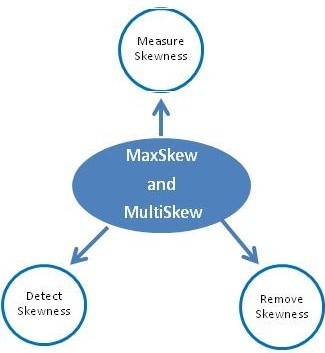
MaxSkew and
MultiSkew provide an unified treatment of multivariate skewness by detecting, measuring and alleviating skewness from multivariate data. Data visualization and significance levels are used to assess the hypothesis of symmetry. Default measures of multivariate skewness depend on third-order moments of the standardized distribution. Linear projections might remove or at least alleviate multivariate skewness. To the best of our knowledge, no statistical packages compute their bootstrap estimates, the third cumulant and linear projections alleviating skewness.
MaxSkew and
Multiskew were released in 2017. Since then, there has been a lot of research on flexible multivariate distributions purported to model nonnormal features such as skewness. Their third cumulants do not necessarily have simple analytical expressions and might need to be investigated by means of simulations studies based on MaxSkew and MultiSkew. The remainder of the paper is organized as follows.
Section 2 reviews the basic concepts of multivariate skewness within the frameworks of third moments and projection pursuit. It also describes some skewness-related features of the Iris dataset.
Section 3 illustrates the package
MaxSkew.
Section 4 describes the functions of
MultiSkew related to symmetrization, third moments and skewness measures.
Section 5 contains some concluding remarks and hints for improving the packages.
2. Third Moment
The third multivariate moment, that is the third moment of a random vector, naturally generalizes to the multivariate case the third moment
of a random variable
X whose third absolute moment is finite. It is defined as follows, for a
d-dimensional random vector
satisfying
, for
. The third moment of
is the
matrix
where “⊗” denotes the Kronecker product (see, for example, [
29,
35]). In the following, when referring to the third moment of a random vector, we shall implicitly assume that all appropriate moments exist.
The third moment
of
contains
elements of the form
, where
, ⋯,
d. Many elements are equal to each other, due to the identities
First, there are at most d distinct elements where the three indices are equal to each other: , for , ⋯, d. Second, there are at most distinct elements where only two indices are equal to each other: , for , ⋯, d and . Third, there are at most distinct elements where the three indices differ from each other: , for , ⋯, d and . Hence contains at most distinct elements.
Invariance of
with respect to indices permutations implies several symmetries in the structure of
. First,
might be regarded as
d matrices
, (
) stacked on top of each other. Hence
is the element in the
j-th row and in the
h-th column of the
i-th block
of
. Similarly,
might be regarded as
d vectorized, symmetric matrices lined side by side:
. Also, left singular vectors corresponding to positive singular values of the third multivariate moment are vectorized, symmetric matrices ([
29]). Finally,
might be decomposed into the sum of at most
d Kronecker products of symmetric matrices and vectors ([
29]).
Many useful properties of multivariate moments are related to the linear transformation
, where
is a
real matrix. The first moment (that is the mean) of
is evaluated via matrix multiplication only:
. The second moment of
is evaluated using both the matrix multiplication and transposition:
where
denotes the second moment of
. The third moment of
is evaluated using the matrix multiplication, transposition and the tensor product:
([
3]). In particular, the third moment of the linear projection
, where
is a
d-dimensional real vector, is
and is a third-order polynomial in the variables
, ...,
.
The third central moment of
, also known as its third cumulant, is the third moment of
, where
is the mean of
:
It is related to the third moment via the identity
The third cumulant allows for a better assessment of skewness by removing the effect of location on third-order moments. It becomes a null matrix under central symmetry, that is when and are identically distributed.
The third standardized moment (or cumulant) of the random vector
is the third moment of
, where
is the inverse of the positive definite square root
of
, which is assumed to be positive definite:
It is often denoted by
and is related to
via the identity
The third standardized cumulant is particularly useful for removing the effects of location, scale and correlations on third order moments. The mean and the variance of are invariant with respect to orthogonal transformations, but the same does not hold for third moments: and may differ, if and is a orthogonal matrix.
Projection pursuit is a multivariate statistical technique aimed at finding interesting low-dimensional data projections. It looks for the data projections which maximize the projection pursuit index, that is a measure of interestingness. [
18] reviews the merits of skewness (i.e., the third standardized cumulant) as a projection pursuit index. Skewness-based projection pursuit is based on the multivariate skewness measure in [
28]. They defined the directional skewness of a random vector
as the maximum value
attainable by
, where
is a nonnull,
d-dimensional real vector and
is the Pearson’s skewness of the random variable
Y:
with
being the set of
d-dimensional real vectors of unit length. The name directional skewness reminds that
is the maximum skewness attainable by a projection of the random vector
onto a direction. It admits a simple representation in terms of the third standardized cumulant:
Statistical applications of directional skewness include normality testing ([
28]), point estimation ([
36]), independent component analysis ([
6,
29]) and cluster analysis ([
4,
9,
10,
11,
12,
18]).
There is a general consensus that an interesting feature, once found, should be removed ([
37,
38]). In skewness-based projection pursuit, this means removing skewness from the data using appropriate linear transformations. A random vector whose third cumulant is a null matrix is said to be weakly symmetric. Weak symmetry might be achieved by linear transformations: any random vector with finite third-order moments and at least two components admits a projection which is weakly symmetric ([
34]).
The appropriateness of the linear transformation purported to remove or alleviate symmetry might be assessed with measures of multivariate skewness, which should be significantly smaller in the transformed data than in the original ones. Ref. [
24] summarized the multivariate skewness of the random vector
with the scalar measure
where
and
are two
d-dimensional, independent and identically distributed random vectors with mean
and covariance
. It might be represented as the squared norm of the third standardized cumulant:
It is invariant with respect to one-to-one affine transformations:
Mardia’s skewness is by far the most popular measure of multivariate skewness. Its statistical applications include multivariate normality testing ([
24]) and the robustness of MANOVA statistics ([
25]).
Another scalar measure of multivariate skewness is
where
and
are the same as above. It has been independently proposed by several authors ([
25,
26,
27]). Ref. [
29] named it partial skewness to remind that
does not depend on moments of the form
when
i,
j,
h differ from each other, as it becomes apparent when representing it as a function of the third standardized cumulant:
Partial skewness is by far less popular than Mardia’s skewness. Like the latter measure, however, it has been applied to multivariate normality testing ([
39,
40,
41]) and for assessing the robustness of MANOVA statistics ([
25]).
Ref. [
27] proposed to measure the skewness of the
d-dimensional random vector
with the vector
, where
is the standardized version of
. This vector-valued measure of skewness might be regarded as weighted average of the standardized vector
, with more weight placed on the outcomes furthest away from the sample mean. It is location invariant, admits the representation
and its squared norm is the partial skewness of
. It coincides with the third standardized cumulant of a random variable in the univariate case, and with the null
d-dimensional vector when the underlying distribution is centrally symmetric. [
11] applied it to model-based clustering.
We shall illustrate the role of skewness with the Iris dataset contained in the R package datasets: iris{datasets}. We shall first download the data: R> data(iris). Then use the help command R>help(iris) and the structure command R> str(iris) to obtain the following information about this dataset. It contains the measurements in centimeters of four variables on 150 iris flowers: sepal length, sepal width, petal length and petal width. There is also a factor variable (Species) with three levels: setosa, versicolor and virginica. There are 50 rows for each species. The output of the previous code shows that the dataset is a data frame object containing 150 units and five variables:
‘data.frame’: 150 obs. of 5 variables:
$ Sepal.Length: num 5.1 4.9 4.7 4.6 5 5.4 4.6 5 4.4 ...
$ Sepal.Width : num 3.5 3 3.2 3.1 3.6 3.9 3.4 3.4 2.9 ...
$ Petal.Length: num 1.4 1.4 1.3 1.5 1.4 1.7 1.4 1.5 1.4 ...
$ Petal.Width : num 0.2 0.2 0.2 0.2 0.2 0.4 0.3 0.2 0.2 ...
$ Species : Factor w/ 3 levels "setosa","versicolor",..: 1 1...
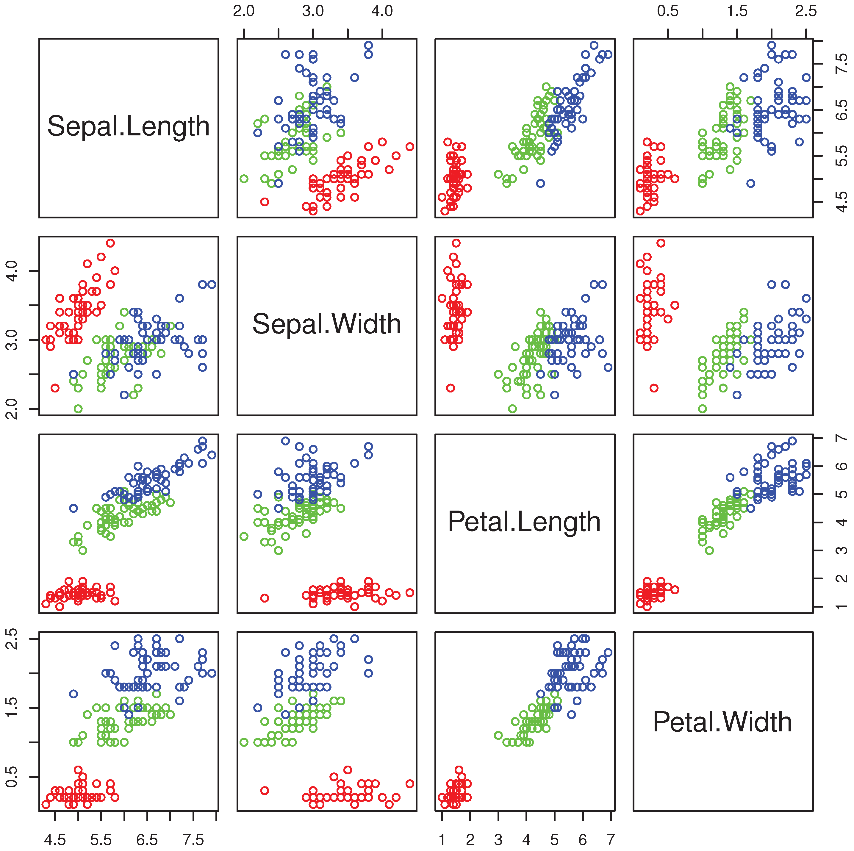
With the command
R> pairs(iris[,1:4],col=c("red","green","blue")[as.numeric(Species)]) we obtain the multiple scatterplot of the Iris dataset (
Figure 1).
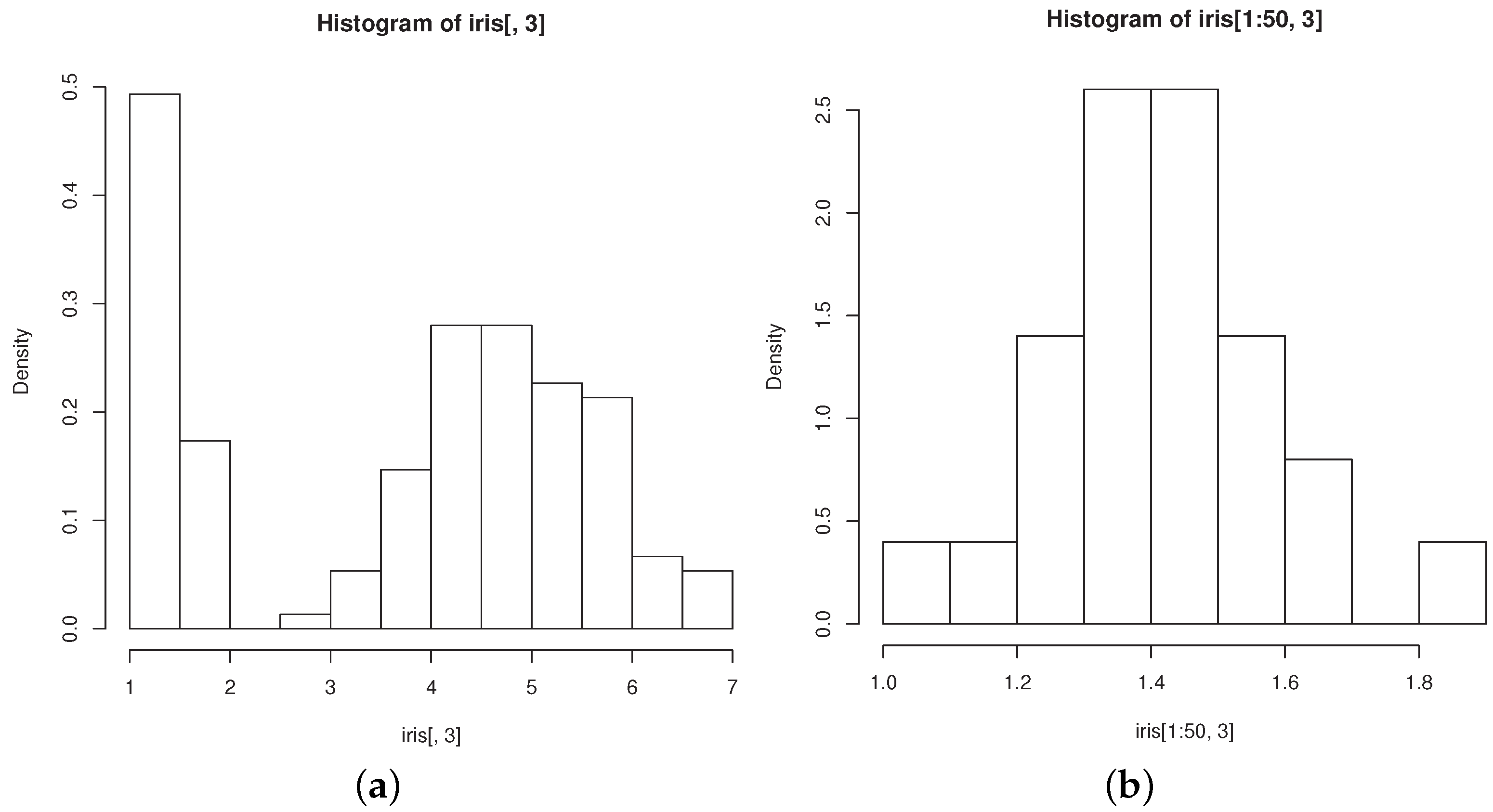
The groups “versicolor” and “virginica” are quite close to each other and well separated from “setosa”. The data are markedly skewed, but skewness reduces within each group, as exemplified by the histograms of petal length in all flowers (
Figure 2a) and in those belonging to the “setosa” group (
Figure 2b). Both facts motivated researchers to model the dataset with mixtures of three normal components (see, for example [
42], Section 6.4.3). However, [
43] showed that the normality hypothesis should be rejected at the
level in the “setosa” group, while nonnormality is undetected by Mardia’s skewness.
We shall use MaxSkew and MultiSkew to answer the following questions about the Iris dataset.
Is skewness really inept at detecting nonnormality of the variables in the “setosa” group?
Does skewness help in recovering the cluster structure?
Can skewness be removed via meaningful linear projections?
The above questions will be addressed within the frameworks of projection pursuit, normality testing, cluster analysis and data exploration.
3. MaxSkew
The package
MaxSkew uses several
R functions. The first one is
[
45]. It computes eigenvalues and eigenvectors of real or complex matrices. Its usage, as described by the command
help(eigen) is
R> eigen(x, symmetric, only.values = FALSE, EISPACK = FALSE).
The output of the function are
values (a vector containing the eigenvalues of
x, sorted in decreasing order according to their modulus) and
vectors (either a matrix whose columns contain the normalized eigenvectors of
x, or a null matrix if
only.values is set equal to TRUE). A second
R function used in
MaxSkew is
[
45] which finds the zeros of a real or complex polynomial. Its usage is
polyroot(z), where
z is the vector of polynomial coefficients arranged in increasing order. The
Value in output is a complex vector of length
, where
n is the position of the largest non-zero element of
z.
MaxSkew also uses the
R function
[
45] which computes the singular value decomposition of a matrix. Its usage is
R> svd(x, nu = min(n, p), nv = min(n, p), LINPACK = FALSE).
The last
R function used in
MaxSkew is
[
45] which computes the Kronecker product of two arrays,
X and
Y. The
Value in output is an array with dimensions
dim(X) * dim(Y).
The
MaxSkew package finds orthogonal data projections with maximal skewness. The first data projection in the output is the most skewed among all data projections. The second data projection in the output is the most skewed among all data projections orthogonal to the first one, and so on. Ref. [
4] motivates this method within the framework of model-based clustering. The package implements the algorithm described in [
18] and is downloaded with the command
R> install.packages(“MaxSkew”). The package is attached with the command
R > library(MaxSkew).
The packages MaxSkew and MultiSkew require the dataset to be a data matrix object, so we transform the iris data frame accordingly: R > iris.m<-data.matrix(iris). We check that we have a data matrix object with the command
R > str(iris.m)
num [1:150, 1:5] {5.1} {4.9} {4.7} {4.6 } {5} {5.4} {...}
- attr(*, "dimnames")=List of 2
..$ : NULL
..$ : chr [1:5] "Sepal.Length" "Sepal.Width" "Petal.Length"
"Petal.Width" ...
The help command shows the basic informations about the package and the functions it contains: R > help(MaxSkew).
The package MaxSkew has three functions, two of which are internal. The usage of the main function is
R> MaxSkew(data, iterations, components, plot),
where data is a data matrix object, iterations (the number of required iterations) is a positive integer, components (the number of orthogonal projections maximizing skewness) is a positive integer smaller than the number of variables, and plot is a dichotomous variable: TRUE/FALSE. If plot is set equal to TRUE (FALSE) the scatterplot of the projections maximizing skewness appears (does not appear) in the output. The output includes a matrix of projected data, whose i-th row represents the i-th unit, while the j-th column represents the j-th projection. The output also includes the multiple scatterplot of the projections maximizing skewness. As an example, we call the function
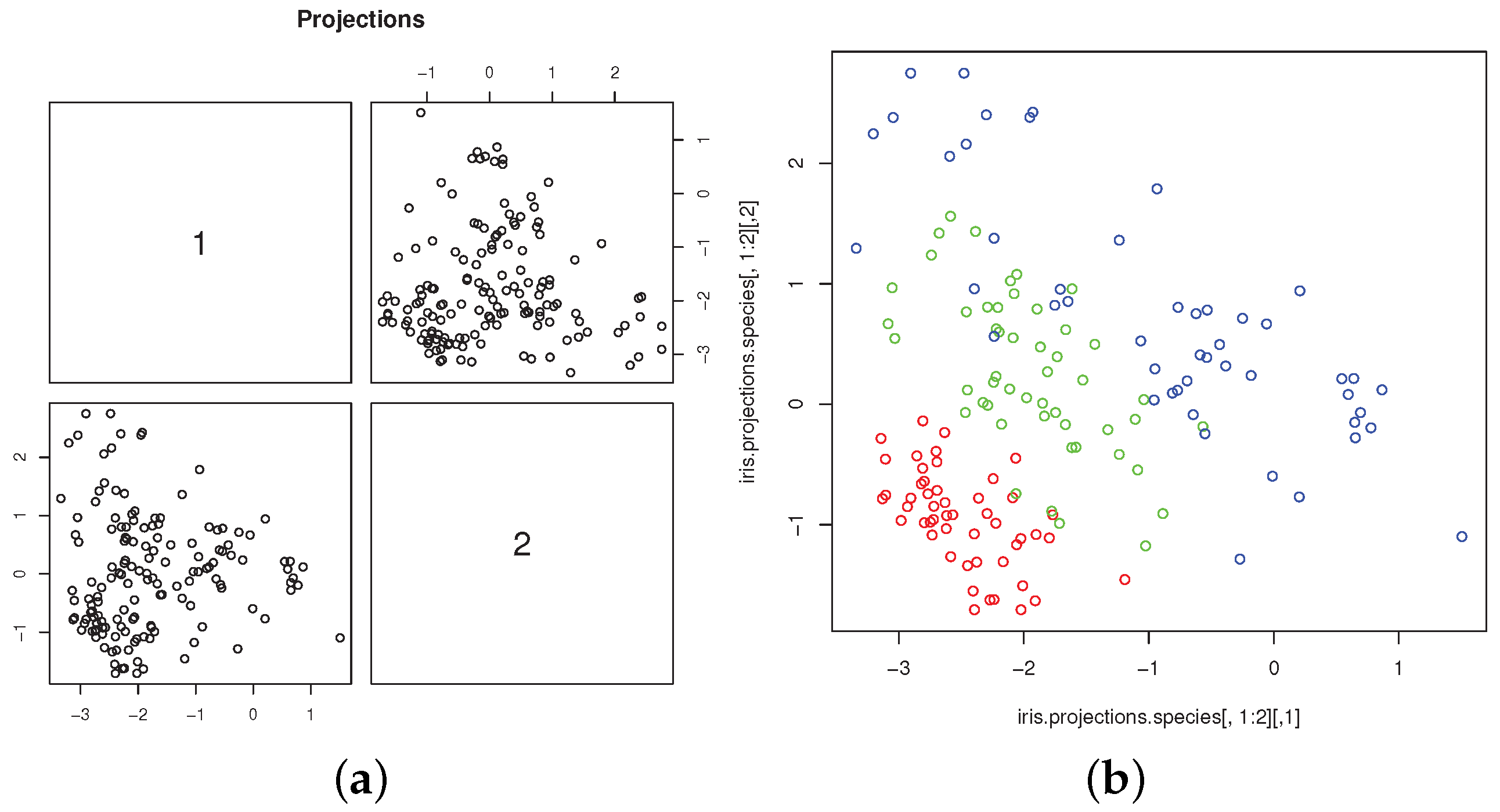
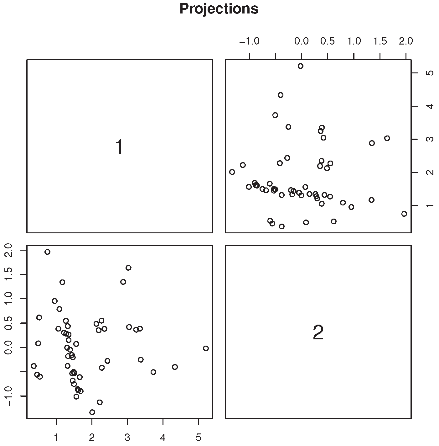
R > MaxSkew(iris.m[,1:4], 50, 2, TRUE).
We have used only the first four columns of the iris.m data matrix object, because the last column is a label. As a result, we obtain a matrix with 150 rows and 2 columns containing the projected data and a multiple scatterplot. The structure of the resulting matrix is
R> str(MaxSkew(iris.m[,1:4], 50, 2, TRUE))
num [1:150, 1:2] −2.63 −2.62 −2.38 −2.58 −2.57 ...
For the sake of brevity we show only the first three rows of the projected data matrix:
R > iris.projections<−MaxSkew(iris.m[,1:4], 50,2,TRUE)
R > iris.projections[1:3,]
[,1] [,2]
[1,] −2.631244186 −0.817635353
[2,] −2.620071890 −1.033692782
[3,] −2.376652037 −1.311616693
Figure 3a shows the scatterplot of the projected data. The connections between skewness-based projection pursuit and cluster analysis, as implemented in
MaxSkew, have been investigated by several authors ([
4,
9,
10,
11,
12,
18]). For the Iris dataset, it is well illustrated by the scatterplot of the two most skewed, mutually orthogonal projections, with different colors to denote the group memberships (
Figure 3b). The plot is obtained with the commands
R> attach(iris)
R> iris.projections<−MaxSkew(iris.m[,1:4], 50,2,TRUE)
R> iris.projections.species<−cbind(iris.projections,
iris$Species)
R> pairs(iris.projections.species[,1:2],
col=c("red","green","blue")[as.numeric(Species)])
R>detach(iris)
The scatterplot clearly shows the separation of “setosa” from “virginica” and “versicolor”, whose overlapping is much less marked than in the original variables. The scatterplot is very similar, up to rotation and scaling, to those obtained from the same data by [
46,
47].
Mardia’s skewness is unable to detect nonnormality in the “setosa” group, thus raising the question of whether any skewness measure is apt at detecting such nonnormality ([
43]). We address this question using skewness-based projection pursuit as a visualization tool.
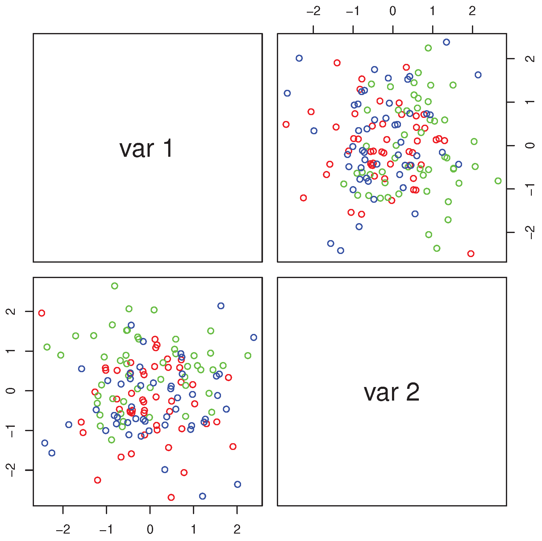
Figure 4 contains the scatterplot of the two most skewed, mutually orthogonal projections obtained from the four variables recorded from setosa flowers only. It clearly shows the presence of a dense, elongated cluster, which is inconsistent with the normality assumption. Formal testing for excess skewness in the “setosa” group will be discussed in the following sections.
4. MultiSkew
The package
MultiSkew ([
48]) is written in the
R programming language [
45] and depends on the recommended package
MaxSkew ([
44]). It is available for download on the Comprehensive
R Archive Network (CRAN) at
https://CRAN.R-project.org/package=MultiSkew. The
MultiSkew package computes the third multivariate cumulant of either the raw, centered or standardized data. It also computes the main measures of multivariate skewness, together with their bootstrap distributions. Finally, it computes the least skewed linear projections of the data. The
MultiSkew package contains six different functions. First install it with the command
R> install.packages(“MultiSkew”) and then use the command
R > library(MultiSkew) to attach the package. Since the package
MultiSkew depends on the package
MaxSkew, the latter is loaded together with the former.
4.1. MinSkew
The function
R > MinSkew(data, dimension) alleviates sample skewness by projecting the data onto appropriate linear subspaces and implements the method in [
34]. It requires two input arguments:
data (a data matrix object), and
dimension (the number of required projections), which must be an integer between 2 and the number of the variables in the data matrix. The output has two values:
Linear (the linear function of the variables) and
Projections (the projected data).
Linear is a matrix with the number of rows and columns equal to the number of variables and number of projections.
Projections is a matrix whose number of rows and columns equal the number of observations and the number of projections. We call the function using our data matrix object:
R > MinSkew(iris.m[,1:4],2). We obtain the matrix
Linear as a first output. With the commands
R> attach(iris)
R> projections.species<−cbind(Projections,iris$Species)
R> pairs(projections.species[,1:2],col=c("red","green",
"blue")[as.numeric(Species)])
R> detach(iris)
we obtain the multiple scatterplot of the two projections (
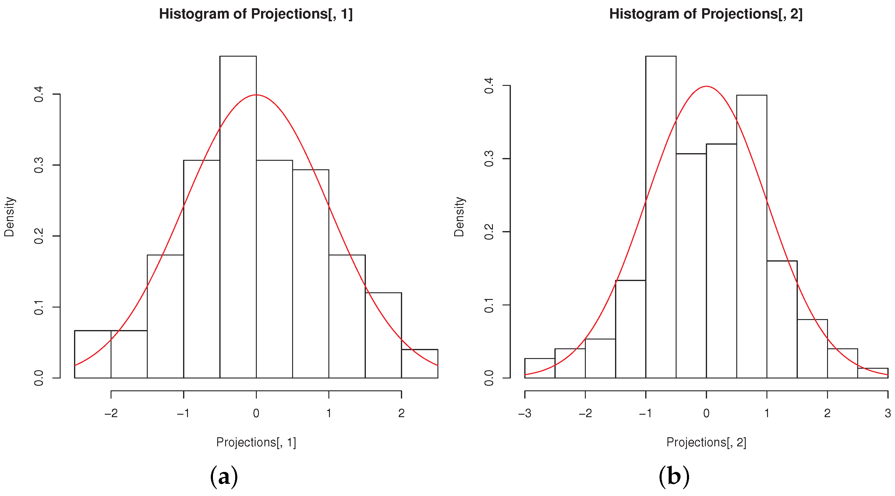
Figure 5). The points clearly remind of bivariate normality and the groups markedly overlap with each other. Hence the projection removes the group structure as well as skewness. This result might be useful for a researcher interested in the features which are common to the three species.
The histograms of the
MinSkew projections remind of univariate normality, as it can be seen from
Figure 6a,b, obtained with the code
R> hist(Projections[,1],freq=FALSE)
R> curve(dnorm, col = 2, add = TRUE)
R> hist(Projections[,2],freq=FALSE)
R> curve(dnorm, col = 2, add = TRUE)
4.2. Third
This section describes the function which computes the third multivariate moment of a data matrix. Some general information about the third multivariate moment of both theoretical and empirical distributions are reviewed in [
29]. The name of the function is
Third, and its usage is
R > Third(data,type).
As before, data is a data matrix object while type may be: “raw” (the third raw moment), “central” (the third central moment) and “standardized” (the third standardized moment). The output of the function, called ThirdMoment, is a matrix containing all moments of order three which can be obtained from the variables in data. We compute the third raw moments of the numerical variables in the iris dataset with the command R > Third(iris.m[,1:4], “raw”). The matrix ThirdMoment is:
[1] "Third Moment"
[,1] [,2] [,3] [,4]
[1,] 211.6333 106.0231 145.8113 47.7868
[2,] 106.0231 55.4270 69.1059 22.3144
[3,] 145.8113 69.1059 109.9328 37.1797
[4,] 47.7868 22.3144 37.1797 12.9610
[5,] 106.0231 55.4270 69.1059 22.3144
[6,] 55.4270 30.3345 33.7011 10.6390
[7,] 69.1059 33.7011 50.7745 17.1259
[8,] 22.3144 10.6390 17.1259 5.9822
[9,] 145.8113 69.1059 109.9328 37.1797
[10,] 69.1059 33.7011 50.7745 17.1259
[11,] 109.9328 50.7745 86.4892 29.6938
[12,] 37.1797 17.1259 29.6938 10.4469
[13,] 47.7868 22.3144 37.1797 12.9610
[14,] 22.3144 10.6390 17.1259 5.9822
[15,] 37.1797 17.1259 29.6938 10.4469
[16,] 12.9610 5.9822 10.4469 3.7570
Similarly, we use "central" instead of "raw" with the command R > Third(iris.m[,1:4], "central"). The output which appears in console is
[1] "Third Moment"
[,1] [,2] [,3] [,4]
[1,] 0.1752 0.0420 0.1432 0.0259
[2,] 0.0420 −0.0373 0.1710 0.0770
[3,] 0.1432 0.1710 −0.1920 −0.1223
[4,] 0.0259 0.0770 −0.1223 −0.0466
[5,] 0.0420 −0.0373 0.1710 0.0770
[6,] −0.0373 0.0259 −0.1329 −0.0591
[7,] 0.1710 −0.1329 0.5943 0.2583
[8,] 0.0770 −0.0591 0.2583 0.1099
[9,] 0.1432 0.1710 −0.1920 −0.1223
[10,] 0.1710 −0.1329 0.5943 0.2583
[11,] −0.1920 0.5943 −1.4821 −0.6292
[12,] −0.1223 0.2583 −0.6292 −0.2145
[13,] 0.0259 0.0770 −0.1223 −0.0466
[14,] 0.0770 −0.0591 0.2583 0.1099
[15,] −0.1223 0.2583 −0.6292 −0.2145
[16,] −0.0466 0.1099 −0.2145 −0.0447
and the structure of the object ThirdMoment is
Finally, we set type equal to standardized: R > Third(iris.m[,1:4], "standardized"). The output is
[1] "Third Moment"
[,1] [,2] [,3] [,4]
[1,] 0.2988 −0.0484 0.3257 0.0034
[2,] −0.0484 0.0927} −0.0358 −0.0444
[3,] 0.3257 −0.0358} 0.0788 −0.2221
[4,] 0.0034 −0.0444} −0.2221 0.0598
[5,] −0.0484 0.0927} −0.0358 −0.0444
[6,] 0.0927 −0.0331} −0.1166 −0.0844
[7,] −0.0358 −0.1166} 0.2894 0.1572
[8,] −0.0444 −0.0844} 0.1572 0.2276
[9,] 0.3257 −0.0358} 0.0788 −0.2221
[10,] −0.0358 −0.1166} 0.2894 0.1572
[11,] 0.0788 0.2894} −0.0995 −0.3317
[12,] −0.2221 0.1572} −0.3317 0.3009
[13,] 0.0034 −0.0444} −0.2221 0.0598
[14,] −0.0444 −0.0844} 0.1572 0.2276
[15,] −0.2221 0.1572} −0.3317 0.3009
[16,] 0.0598 0.2276} 0.3009 0.8259
We show the structure of the matrix ThirdMoment with
Third moments and cumulants might give some insights into the data structure. As a first example, use the command
R> Third(MaxSkew(iris.m[1:50,1:4],50,2,TRUE),"standardized")
to compute the third standardized cumulant of the two most skewed, mutually orthogonal projections obtained from the four variables recorded from setosa flowers only. The resulting matrix is
[1] "Third Moment"
[,1] [,2]
[1,] 1.2345 0.0918
[2,] 0.0918 −0.0746
[3,] 0.0918 −0.0746
[4,] −0.0746 0.5936
The largest entries in the matrix are the first element of the first row and the last element in the last row. This pattern is typical of outcomes from random vectors with skewed, independent components (see, for example, [
29]). Hence the two most skewed projections might be mutually independent. As a second example, use the commands
R> MinSkew(iris.m[,1:4],2) and R> Third(Projections,“standardized”),
where Projections is a value in output of the function MinSkew, to compute the third standardized cumulant of the two least skewed projections obtained from the four numerical variables of the Iris dataset. The resulting matrix is
[,1] [,2]
[1,] −0.0219 0.0334
[2,] 0.0334 −0.0151
[3,] 0.0334 −0.0151
[4,] −0.0151 −0.0963
All elements in the matrix are very close to zero, as it might be better appreciated by comparing them with those in the third standardized cumulant of the original variables. This pattern is typical of outcomes from weakly symmetric random vectors ([
34]).
4.3. Skewness Measures
The package MultiSkew has other four functions. All of them compute skewness measures. The first one is R > FisherSkew(data) and computes Fisher’s measure of skewness, that is the third standardized moment of each variable in the dataset. The usage of the function shows that there is only one input argument: data (a data matrix object). The output of the function is a dataframe, whose name is tab, containing Fisher’s measure of skewness of each variable of the dataset. To illustrate the function, we use the four numerical variables in the Iris dataset with the command R > FisherSkew(iris.m[,1:4]) and obtain the output
in which
X1 is the variable Sepal.Length,
X2 is the variable Sepal.Width,
X3 is the variable Petal.Length, and
X4 is the variable Petal.Width. Another function is
PartialSkew: R > PartialSkew(data). It computes the multivariate skewness measure as defined in [
27]. The input is still a data matrix, while the values in output are the objects
Vector, Scalar and
pvalue. The first is the skewness measure and it has a number of elements equal to the number of the variables in the dataset used as input. The second is the squared norm of
Vector. The last is the probability of observing a value of
Scalar greater than the observed one, when the data are normally distributed and the sample size is large enough. We apply this function to our dataset:
R > PartialSkew(iris.m[,1:4]) and obtain
R > Vector
[,1]
[1,] 0.5301
[2,] 0.4355
[3,] 0.4105
[4,] 0.4131
R > Scalar
[,1]
[1,] 0.8098
R > pvalue
[,1]
[1,] 0.0384
The function
R > SkewMardia(data) computes the multivariate skewness introduced in [
24], that is the sum of squared elements in the third standardized cumulant of the data matrix. The output of the function is the squared norm of the third cumulant of the standardized data (
MardiaSkewness) and the probability of observing a value of
MardiaSkewness greater than the observed one, when data are normally distributed and the sample size is large enough (
pvalue). With the command
R > SkewMardia(iris.m[,1:4]) we obtain
R > MardiaSkewness
[1] 2.69722
R > pvalue
[1] 4.757998e−07
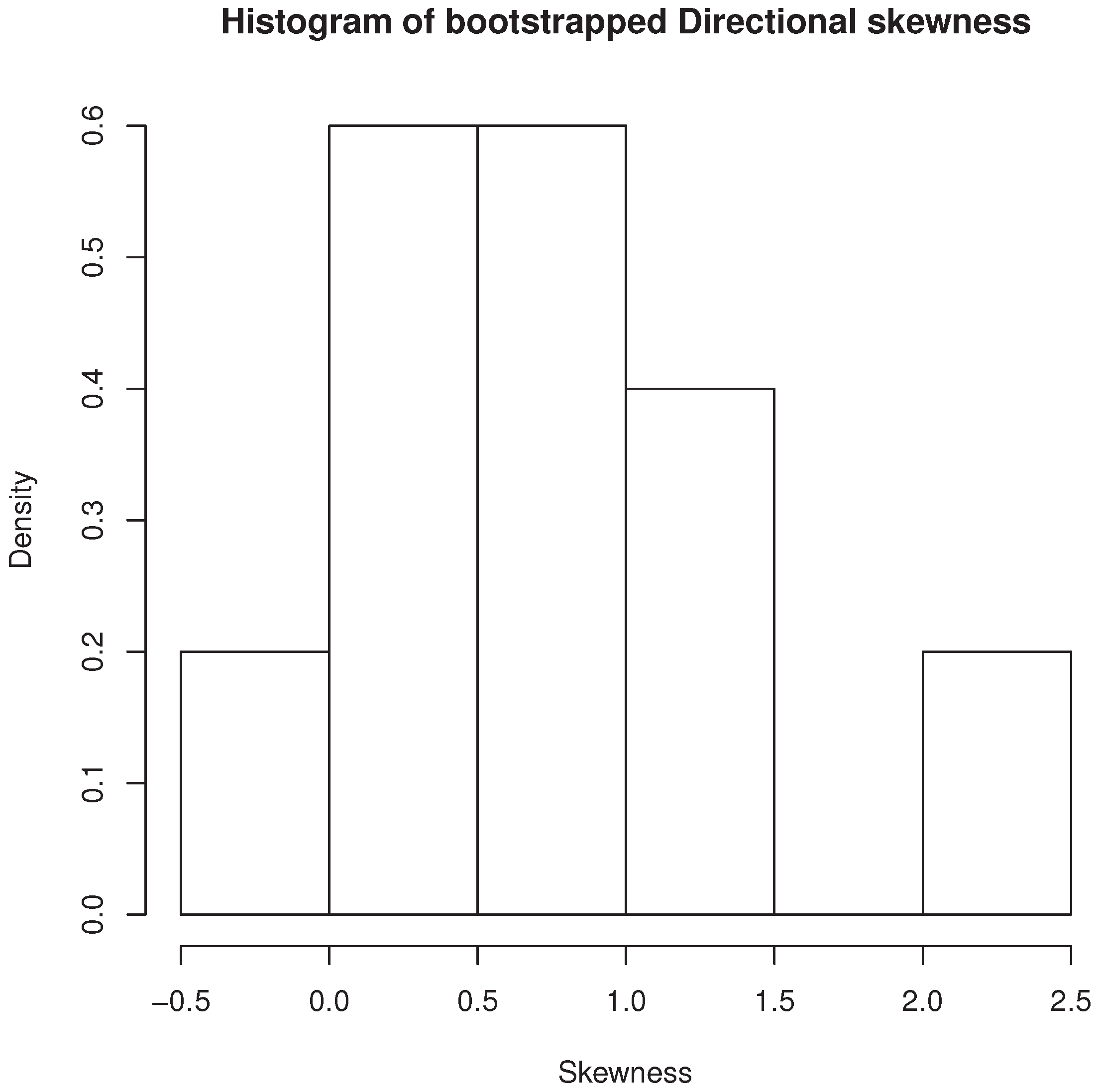
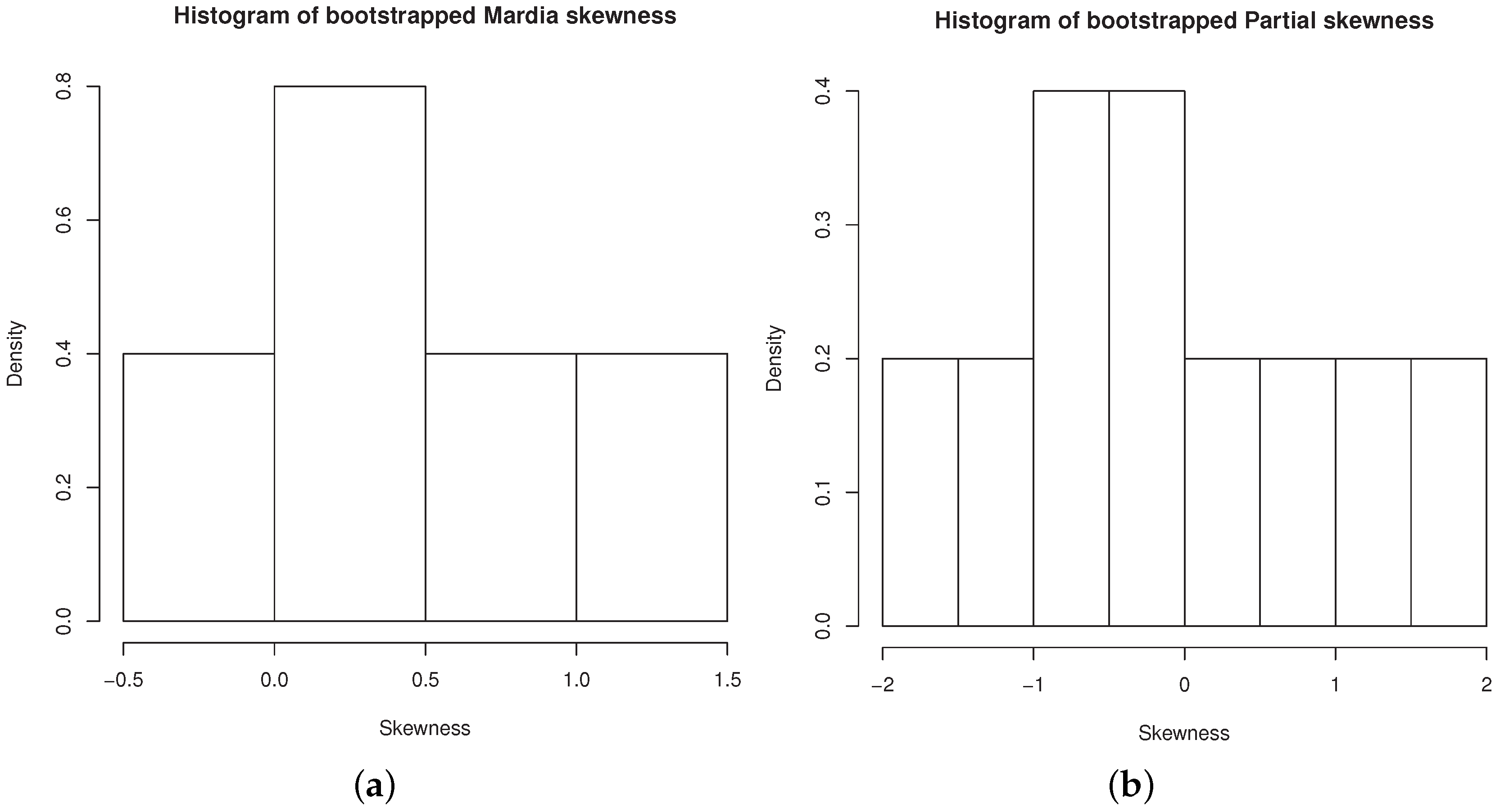
The function SkewBoot performs bootstrap inference for multivariate skewness measures. It computes the bootstrap distribution, its histogram and the p-value of the chosen measure of multivariate skewness using a given number of bootstrap replicates. The function calls the function MaxSkew contained in MaxSkew package, with the number of iterations required by the function MaxSkew set equal to 5. The function’s usage is R > SkewBoot(data, replicates, units, type). It requires four inputs: data (the data matrix object), replicates (the number of bootstrap replicates), units (the number of rows in the data matrices sampled from the original data matrix object) and type. The latter may be “Directional”, “Partial” or “Mardia” (three different measures of multivariate skewness). If type is set equal to “Directional” or “Mardia”, units is an integer greater than the number of variables. If type is set equal to “Partial”, units is an integer greater than the number of variables augmented by one. The values in output are three: histogram (a plot of the above mentioned bootstrap distribution), Pvalue (the p-value of the chosen skewness measure) and Vector (the vector containing the bootstrap replicates of the chosen skewness measure). For the reproducibility of the result, before calling the function SkewBoot, we type R> set.seed(101) and then R > SkewBoot(iris.m[,1:4],10,11,“Directional”). We obtain the output
and also the histogram of bootstrapped directional skewness (
Figure 7).
We call the function SkewBoot, first setting type equal to Mardia and then equal to Partial:
R> set.seed(101)
R > SkewBoot(iris.m[,1:4],10,11,"Mardia").
We obtain the output
[1] "Vector"
[1] 1.4768 1.1260 0.8008 0.6164 0.4554 0.1550 0.0856
−0.1394 −0.1857 0.4018
[1] "Pvalue"
[1] 0.6363636
R> set.seed(101)
R > SkewBoot(iris.m[,1:4],10,11,"Partial"),
[1] "Vector"
[1] 1.5435 1.0110 0.6338 0.2858 −0.0053 −0.3235 −0.6701
-1.1134 −1.7075 −0.9563
[1] "Pvalue"
[1] 0.3636364
Figure 8a,b contain the histograms of bootstrapped Mardia’s skewness and bootstrapped partial skewness, respectively.
We shall now compute the Fisher’s skewnesses of the four variables in the “setosa” group with
R > FisherSkew(iris.m[1:50,1:4]). The output is the dataframe
Ref. [
43] showed that nonnormality of variables in the “setosa” group went undetected by Mardia’s skewness calculated on all four of them (the corresponding
p-value is 0.1772). We compute Mardia’s skewness of the two most skewed variables (sepal length and petal width), with the commands
R>iris.m.mardia<-cbind(iris.m[1:50,1],iris.m[1:50,4])
R>SkewMardia(iris.m.mardia).
We obtain the output
R> MardiaSkewness
[1] 1.641217
R> pvalue
[1] 0.008401288
The p-value is highly significant, clearly suggesting the presence of skewness and hence of nonnormality. We conjecture that the normality test based on Mardia’s skewness is less powerful when skewness is present only in a few variables, either original or projected, while the remaining variables might be regarded as background noise. We hope to either prove or disprove this conjecture by both theoretical results and numerical experiments in future works.


