Fast Color Quantization by K-Means Clustering Combined with Image Sampling

Abstract

Color image quantization has become an important operation often used in tasks of color image processing. There is a need for quantization methods that are fast and at the same time generating high quality quantized images. This paper presents such color quantization method based on downsampling of original image and K-Means clustering on a downsampled image. The nearest neighbor interpolation was used in the downsampling process and Wu’s algorithm was applied for deterministic initialization of K-Means. Comparisons with other methods based on a limited sample of pixels (coreset-based algorithm) showed an advantage of the proposed method. This method significantly accelerated the color quantization without noticeable loss of image quality. The experimental results obtained on 24 color images from the Kodak image dataset demonstrated the advantages of the proposed method. Three quality indices (MSE, DSCSI and HPSI) were used in the assessment process.

1. Introduction

Color image quantization plays an auxiliary, but still very important role in such tasks of color image processing as image compression, image segmentation, image watermarking, etc. This operation significantly reduces the number of colors in the image and at the same time it should maintain a quantized image similar to the original image. Among the color quantization methods, two large groups can be distinguished, i.e., splitting techniques, e.g., median-cut (MC) [1], Wu’s algorithm [2] and clustering techniques, e.g., K-Means (KM) technique [3]. The latter technique gives very good results, but its computational complexity makes for a long computation time.

The results obtained using the KM technique depend on the initialization, i.e., on how we determine the initial centers of the clusters. Their random selection, usually used in the KM technique, leads to unrepeatable results. The use of splitting quantization in the form of MC or Wu methods can provide a deterministic initialization of KM [4].

The high computational complexity of KM results from the necessity of carrying out a very large number of comparisons between input data. This is especially true for images that contain millions of pixels. Therefore, the use of appropriate data structures and reducing the number of unnecessarily calculated distances between data allows for reducing the time required for KM [5]. Another approach, particularly useful in color quantization, can be the operation on a small sample of the image. Then, the problem of how to sample the image remains to be solved: randomly or systematically? The other challenge is to define a proper size of such sample to receive accurate results and shorter computational time [6]. In this paper by Bejarano et al., the maximal size of the sample was about 0.5% of the entire data and the clustering results were accurate and achieved in a much shorter time. A reduction in the number of pixels reduced the number of unique colors and then we could carry out the color quantization, for example, on a few thousand colors, not on a few million colors. The result should be a small loss of image quality and a significantly shorter time for the whole operation. The three main contributions of the proposed method are as follows:

• An improved color quantization method may result in high image quality and short quantization time simultaneously.
• Our method limits its working area to the stage of determining the color palette (initialization, clustering) to the image downsampled by the Nearest Neighbor Interpolation (NNI).
• The quality indices of our quantized images compared with results for the method based on a limited sample of pixels (coreset-based algorithm) show an advantage of our method.

This paper is organized as follows: Section 2 is a short review of the literature on the applications related to the simultaneous color quantization and image downsampling. The proposed method is elaborated in details in Section 3. Experimental results and performance analyses are presented in Section 4. Finally, conclusions are given in Section 5.

2. Related Work

A theoretical basis for solving our problem is the image interpolation. This operation occurs during some image processing stages such as resizing (resampling), rectification, inpainting and morphing. The problem of image interpolation has been widely described in the work [7]. Commonly used non-adaptive interpolation techniques are nearest neighbor interpolation (NNI), bilinear interpolation and bicubic interpolation. NNI is a simplest interpolation method that just replicates the nearest neighboring pixels. This means that, for color images, as a result of interpolation, no new colors are created. Thus, image upsampling does not increase the number of colors in the image and image downsampling can only reduce the number of colors, but their values will remain unchanged.

Different researchers have focused on using image sampling for acceleration of color quantization processes. In 2002, Papamarkos et al. [8] presented an idea of image downsampling via a fractal scanning technique based on Hilbert’s space-filling curve for their Adaptive Color Reduction (ACR) algorithm. In this paper, the advantages of such fractal scanning in relation to a conventional raster scanning were highlighted. However, the primary goal of this downsampling was to speed up the entire process, especially important in the case of large images.

In 2014, Szilagyi and coworkers [9] preceded the KM-based color quantization by a special preprocessing consisting of static color quantization on about 140,000 colors and the color histogram computation with rejection of the least frequent colors. The key parameter of preprocessing is the percentage of image pixels included in the clustering process. The resignation from 2–5% pixels of the original image reduced the number of colors to 500–5000 colors and shortened the image quantization time (2–3 speedup ratio) without losing the image details.

In the work by Valenzuela, Celebi and Schaefer [10], an accelerated KM version was proposed that utilizes downsampling (decimation) of the input image, a non-deterministic KM++ initialization algorithm, efficient coreset construction and K-Means clustering. The authors used the name coremeans (CM) for their color quantization method. The decimation is the simple transformation of the discrete image, consisting of keeping every n-th sample and rejecting the rest. Two values of the decimation factor $df$ were considered in the article: $\{2,4\}$ and marked as CM2 and CM4. The KM++ algorithm is known from the literature [11]. The coreset was constructed based on a downsampled original image and on the initial set of centers from the KM++ algorithm. The Lucic et al. algorithm [12] was adapted to the coreset construction. Four values of the coreset fraction $cf$ =$1/2$, $3/8$, $1/4$, $1/8$ were tested. In this paper, the CM method tests were performed on only four images. CM was significantly faster than the KM method and produced the quantized images of a similar quality to KM results. A detailed comparison of CM results and the results of the proposed method are given in Section 4.

Color quantization together with image sampling have been applied in pixel art [13], which is reminiscent of the hand-crafted work of pixel artists. Pixel art images, resulting from the automatic conversion of the color input image to a pixelated (iconic) output image, use low spatial resolution and a small color palette. The described conversion procedure contained two parts: SLIC (Simple Linear Iterative Clustering) algorithm that segments the input image into superpixels and an MCDA (Mass Constrained Deterministic Annealing) fuzzy clustering algorithm. As another application of our main operations, namely color quantization and image sampling, we can see a wireless image sensor network with reduced battery consumption in its nodes [14]. This network was used for monitoring natural environment phenomena e.g., bird nest monitoring. Both operations significantly reduced the amount of transferred data between cameras and server and simultaneously reduced the energy consumption. This approach worked as a lossy image compression algorithm. However, compression was limited by the need to maintain a sufficient image quality needed for labeling by domain experts. For authors, the most beneficial color quantization method was quantization with a fixed palette (8, 16, 32 colors) and the bilinear interpolation algorithm for downsampling.

3. The Proposed Method

The main task of this article is to assess the impact of generating a color palette from a sample of image pixels instead of the whole image on the computation time and the quality of quantization. In 2010, Palus and Frackiewicz applied Wu’s splitting method as an effective method for KM initialization [4]. Figure 1 presents an idea of color quantization where an original full resolution image is a starting point for all processes i.e., initialization (Wu’s algorithm), clustering (KM) and final pixel mapping. The time complexity of this quantization method based on K-Means is $O(n·k·d·i)$ [15], where: n is the number of pixels, k is the number of expecting colors, d is the number of color components and i is the number of iterations.

In contrast to this idea, the new proposed method (Figure 2) uses the original image only for pixel mapping. Both stages—initialization and clustering—are working on downsampled (DS) images. For downsampling with a $df$ factor, we decided to use popular and fast nearest neighbor interpolation. Such an approach should significantly reduce computational requirements and shorten the color quantization time. The time complexity of the proposed quantization method based on K-Means with downsampling is $O(df·n·k·d·i)$ [15], where: $df$ is a downsampling factor, n is the number of pixels, k is the number of expecting colors, d is the number of color components and i is the number of iterations. Because the downsampling factor is a fraction, running time is shortened.

Nearest neighbor interpolation is used for an up- or downscaling algorithm in which vertical and horizontal scaling ratios are calculated as:

$$s_x=\frac{w_1}{w_2},s_y=\frac{h_1}{h_2},$$

(1)

where: $w_1,h_1$ are the width and height of an original image, and $w_2,h_2$ are the width and height of the image after enlarging/shrinking. Finally, the results of multiplying $x,y$ coordinates and ratios are rounding to the nearest integer value. In this way, we receive the coordinates of pixels used in the downscaled image.

Wu’s quantization algorithm as a typical splitting method uses a statistical exploration of colors appearing in the original image. It is based on orthogonal bipartitioning and splits the RGB cube into k boxes, but, at each step, the box with the largest color variance is split along the axis that minimizes the sum of the variances on both sides. The author of the algorithm efficiently solved the problem of how to compute three-dimensional color statistics (means and variances) for these boxes. The means of the colors in the final boxes are selected as a color palette. Other details of the algorithm implementation can be found in Ref. [16].

The KM algorithm consists of four stages:

• Initialization of the KM algorithm with cluster centers from Wu’s algorithm,
• For each pixel $x_i$ that represents RGB components, compute its membership $m\left(c_k\right|x_i)$ in each cluster center $c_k$:

  $$m\left(c_k\right|x_i)=\left\{\begin{array}{c}1,\mathrm{if}l=arg\underset{k}{min}{∥x_i-c_k∥}^2,\hfill \\ 0,\mathrm{otherwise},\hfill \end{array}\right.$$

  (2)
• Recompute location of each center $c_k$ from all pixels $x_i$ based on their memberships:

  $$c_k=\frac{{\sum }_{i=1}^{n}m\left(c_k\right|x_i)x_i}{{\sum }_{i=1}^{n}m\left(c_k\right|x_i)},$$

  (3)
• Repeat two former stages until convergence.

All algorithms used in the proposed method were implemented in Visual C++ and the experiments were conducted on a PC computer running under a Windows operating system, with an Intel Core i7 920 @ 2.67 GHz (Santa Clara, CA, USA) and 8 GB RAM.

4. Experimental Results

In this work, two tests were performed to check the quality and efficiency of the proposed fast color quantization method. For each test image, the quantization into 32, 64, 128 and 256 colors was carried out and quality indices and CPU time were calculated. Generating a color palette was performed on all pixels of the image where the downsampling factor was $1/1$ and on eight subsets of pixels obtained by NNI on the original image, where the downsampling factor was: $1/2$, $1/4$, $1/8$, $1/16$, $1/32$, $1/64$, $1/128$ and $1/256$. Finally, nine quantization results were obtained for each test image, each number of colors, the quality indices were calculated and CPU time was measured.

The most popular quality index widely used in the color image quantization is the MSE and the version for color images is defined as:

$$MSE=\frac{1}{3MN}{\displaystyle \sum _{i=1}^M}{\displaystyle \sum _{j=1}^N}\left[{(R_{ij}-R_{ij}^{*})}^2+{(G_{ij}-G_{ij}^{*})}^2+{(B_{ij}-B_{ij}^{*})}^2\right],$$

(4)

where: $MN$ represents the image resolution, $R_{ij},G_{ij}$ and $B_{ij}$ are the color components of the pixel $(i,j)$ in the original image and $R_{ij}^{*},G_{ij}^{*},B_{ij}^{*}$ are the color components of this pixel in the quantized image. This index is the same as the objective function used in the K-Means technique.

In the last few years, many perceptual indices for image quality assessment (IQA) have been developed. A good example of such index is the DSCSI (Directional Statistics based Color Similarity Index) [17], which consists of three steps. The first step is the image transformation from the RGB into the S-CIELAB color space. In a second step, the local features for color similarity are calculated for three color components: hue, chroma and lightness. In this way, we obtain the following six features: the hue mean similarity, the hue dispersion similarity, the chroma mean similarity, the chroma contrast similarity, the lightness contrast similarity and the lightness structural similarity. In the third step, these six features are combined into two scores: the chromatic similarity $S_C$ and achromatic similarity $S_A$, which are directly used in the final DSCSI formula:

$$Q(I,I^{*})=S_A·{\left(S_C\right)}^{\lambda },$$

(5)

where: I—original image, $I^{*}$—distorted image and $\lambda$ is a weighting factor. The smaller the difference between the original and distorted image, the value of DSCSI metric is closer to 1.

The last considered image quality index is named HPSI (Haar wavelet-based Perceptually Similarity Index) [18]. HPSI is based on the coefficients of three stages of a discrete Haar wavelet transform. These coefficients are used for assessment of local similarities between two compared images. This index uses the six simple 2D Haar wavelet filters to detect horizontal and vertical edges. It is built in both local similarity maps (horizontal and vertical) and both weight functions. Additionally, a nonlinear mapping in the form of the logistic function is introduced in the HPSI computation process. The usefulness of both new indices to assess the image quality after color quantization show the current works [19,20,21].

The first test was performed on four color images: Baboon, Lena, Pepper and Pills, which are shown in Figure 3, to compare results with a method based on the coreset sampling [10]. Baboon, Lena and Peppers are the test images with 512 × 512 pixels and the Pills with 800 × 519 pixels. The article, describing coreset sampling in color quanizations by K-Means, presents results of MSE and CPU time for the original image and four downsampled images with the following factors: $1/2$, $3/8$, $1/4$, and $1/8$. The authors used a non-deterministic KM++ initialization method and therefore they present the mean and standard deviation values of the performance measures for each quantized image. The fast quantization method proposed in this article, based on NNI and Wu’s splitting initialization algorithm, allows for obtaining deterministic results.

Table 1. MSE values for 32 colors.

$\mathit{c}\mathit{f},\mathit{d}\mathit{f}$	NNI	CM2	CM4	NNI	CM2	CM4	NNI	CM2	CM4	NNI	CM2	CM4
	Baboon			Lena			Peppers			Pills
1	378	378	378	126	120	120	234	233	233	204	203	203
1/2	379	383	385	124	121	123	233	232	236	210	205	206
1/4	376	382	395	123	122	124	233	234	240	208	205	208
1/8	381	385	398	123	122	125	237	235	244	206	203	208
1/16	392	N/A	N/A	121	N/A	N/A	238	N/A	N/A	207	N/A	N/A
1/32	388	N/A	N/A	123	N/A	N/A	238	N/A	N/A	207	N/A	N/A
1/64	384	N/A	N/A	123	N/A	N/A	237	N/A	N/A	207	N/A	N/A
1/128	412	N/A	N/A	122	N/A	N/A	242	N/A	N/A	207	N/A	N/A
1/256	400	N/A	N/A	132	N/A	N/A	249	N/A	N/A	212	N/A	N/A

,

Table 2. MSE values for 64 colors.

$\mathit{c}\mathit{f},\mathit{d}\mathit{f}$	NNI	CM2	CM4	NNI	CM2	CM4	NNI	CM2	CM4	NNI	CM2	CM4
	Baboon			Lena			Peppers			Pills
1	240	238	238	75	73	73	138	137	137	117	114	114
1/2	241	242	248	73	74	79	140	137	141	115	114	117
1/4	243	243	251	75	74	77	140	138	144	113	115	117
1/8	247	245	258	75	75	79	140	139	146	114	115	121
1/16	243	N/A	N/A	75	N/A	N/A	139	N/A	N/A	113	N/A	N/A
1/32	249	N/A	N/A	75	N/A	N/A	138	N/A	N/A	117	N/A	N/A
1/64	249	N/A	N/A	76	N/A	N/A	142	N/A	N/A	116	N/A	N/A
1/128	256	N/A	N/A	78	N/A	N/A	143	N/A	N/A	120	N/A	N/A
1/256	263	N/A	N/A	80	N/A	N/A	154	N/A	N/A	124	N/A	N/A

,

Table 3. MSE values for 128 colors.

$\mathit{c}\mathit{f},\mathit{d}\mathit{f}$	NNI	CM2	CM4	NNI	CM2	CM4	NNI	CM2	CM4	NNI	CM2	CM4
	Baboon			Lena			Peppers			Pills
1	156	152	152	48	47	47	85	84	84	69	67	67
1/2	157	157	162	48	47	49	85	86	89	68	68	70
1/4	157	158	167	48	48	51	86	87	92	69	68	71
1/8	158	160	172	48	49	52	86	88	94	68	69	73
1/16	157	N/A	N/A	48	N/A	N/A	87	N/A	N/A	68	N/A	N/A
1/32	159	N/A	N/A	49	N/A	N/A	87	N/A	N/A	69	N/A	N/A
1/64	163	N/A	N/A	50	N/A	N/A	90	N/A	N/A	71	N/A	N/A
1/128	172	N/A	N/A	52	N/A	N/A	95	N/A	N/A	73	N/A	N/A
1/256	174	N/A	N/A	54	N/A	N/A	100	N/A	N/A	76	N/A	N/A

and

Table 4. MSE values for 256 colors.

$\mathit{c}\mathit{f},\mathit{d}\mathit{f}$	NNI	CM2	CM4	NNI	CM2	CM4	NNI	CM2	CM4	NNI	CM2	CM4
	Baboon			Lena			Peppers			Pills
1	99	97	97	31	30	30	54	54	54	42	41	41
1/2	100	101	107	31	31	33	54	56	59	42	42	44
1/4	100	103	109	31	32	34	54	57	61	42	43	45
1/8	101	105	114	31	33	35	55	58	63	42	44	47
1/16	102	N/A	N/A	32	N/A	N/A	56	N/A	N/A	42	N/A	N/A
1/32	105	N/A	N/A	32	N/A	N/A	57	N/A	N/A	43	N/A	N/A
1/64	108	N/A	N/A	34	N/A	N/A	59	N/A	N/A	45	N/A	N/A
1/128	113	N/A	N/A	35	N/A	N/A	64	N/A	N/A	47	N/A	N/A
1/256	119	N/A	N/A	38	N/A	N/A	68	N/A	N/A	50	N/A	N/A

show a comparison of the mean MSE values for the two versions of the coreset-based algorithm and for the proposed NNI method in the case of 32, 64,128, and 256 colors, respectively.

Table 5. CPU times for 32 colors.

$\mathit{c}\mathit{f},\mathit{d}\mathit{f}$	NNI	CM2	CM4	NNI	CM2	CM4	NNI	CM2	CM4	NNI	CM2	CM4
	Baboon			Lena			Peppers			Pills
1	345	443	443	124	477	477	154	474	474	828	647	647
1/2	155	1370	116	62	1499	121	79	1327	102	134	3201	233
1/4	201	696	55	40	841	64	50	684	52	49	1634	122
1/8	45	368	57	20	400	31	30	356	28	52	825	68
1/16	15	N/A	N/A	21	N/A	N/A	12	N/A	N/A	16	N/A	N/A
1/32	9	N/A	N/A	13	N/A	N/A	4	N/A	N/A	11	N/A	N/A
1/64	6	N/A	N/A	4	N/A	N/A	2	N/A	N/A	5	N/A	N/A
1/128	2	N/A	N/A	4	N/A	N/A	1	N/A	N/A	3	N/A	N/A
1/256	2	N/A	N/A	2	N/A	N/A	1	N/A	N/A	3	N/A	N/A

,

Table 6. CPU times for 64 colors.

$\mathit{c}\mathit{f},\mathit{d}\mathit{f}$	NNI	CM2	CM4	NNI	CM2	CM4	NNI	CM2	CM4	NNI	CM2	CM4
	Baboon			Lena			Peppers			Pills
1	326	849	849	213	884	844	154	842	842	565	1334	1334
1/2	199	1436	123	249	1513	120	79	1418	129	389	3313	252
1/4	101	754	64	72	798	71	50	759	67	367	1697	138
1/8	34	382	34	34	427	34	30	509	36	146	871	74
1/16	30	N/A	N/A	13	N/A	N/A	12	N/A	N/A	77	N/A	N/A
1/32	18	N/A	N/A	11	N/A	N/A	4	N/A	N/A	21	N/A	N/A
1/64	11	N/A	N/A	10	N/A	N/A	2	N/A	N/A	11	N/A	N/A
1/128	6	N/A	N/A	4	N/A	N/A	1	N/A	N/A	6	N/A	N/A
1/256	3	N/A	N/A	2	N/A	N/A	1	N/A	N/A	3	N/A	N/A

,

Table 7. CPU times for 128 colors.

$\mathit{c}\mathit{f},\mathit{d}\mathit{f}$	NNI	CM2	CM4	NNI	CM2	CM4	NNI	CM2	CM4	NNI	CM2	CM4
	Baboon			Lena			Peppers			Pills
1	471	1706	1706	247	1657	1657	750	1598	1598	800	2492	2492
1/2	233	1584	156	188	1626	150	307	1461	146	486	3484	286
1/4	146	814	79	125	836	89	221	881	76	198	1805	157
1/8	59	434	47	47	488	45	77	411	46	196	950	88
1/16	66	N/A	N/A	31	N/A	N/A	38	N/A	N/A	86	N/A	N/A
1/32	49	N/A	N/A	20	N/A	N/A	32	N/A	N/A	31	N/A	N/A
1/64	17	N/A	N/A	10	N/A	N/A	16	N/A	N/A	16	N/A	N/A
1/128	8	N/A	N/A	5	N/A	N/A	7	N/A	N/A	10	N/A	N/A
1/256	4	N/A	N/A	3	N/A	N/A	3	N/A	N/A	6	N/A	N/A

and

Table 8. CPU times for 256 colors.

$\mathit{c}\mathit{f},\mathit{d}\mathit{f}$	NNI	CM2	CM4	NNI	CM2	CM4	NNI	CM2	CM4	NNI	CM2	CM4
	Baboon			Lena			Peppers			Pills
1	1260	3152	3152	1124	3026	3026	1390	2929	2929	3223	4606	4606
1/2	526	1796	190	339	2137	205	564	1673	186	875	3830	364
1/4	368	898	105	281	1047	111	572	890	98	612	1989	199
1/8	209	522	58	143	575	70	144	490	58	308	1046	108
1/16	93	N/A	N/A	55	N/A	N/A	113	N/A	N/A	243	N/A	N/A
1/32	61	N/A	N/A	35	N/A	N/A	49	N/A	N/A	65	N/A	N/A
1/64	34	N/A	N/A	21	N/A	N/A	29	N/A	N/A	28	N/A	N/A
1/128	11	N/A	N/A	10	N/A	N/A	9	N/A	N/A	25	N/A	N/A
1/256	5	N/A	N/A	4	N/A	N/A	4	N/A	N/A	7	N/A	N/A

contain CPU times for each method in milliseconds. Figure 4 and Figure 5 show the dependencies of the obtained speedup of calculations depending on the value of the downsampling factor for k = 128 and k = 256 where the advantage of the proposed method is significant. The visualization of the results was limited to the cases of k = 128 and k = 256, for which the predominance of the proposed method is the most visible. For cases k = 32 and k = 64, the results are presented in the tables only.

The second test was performed on 24 images from the Kodak image dataset [22] where each standard resolution image is either 768 × 512 pixels or 512 × 768 pixels and they were shown in Figure 6. In addition, the same images of high resolution (3072 × 2048 or 2048 × 3072 pixels) are also available in this dataset.

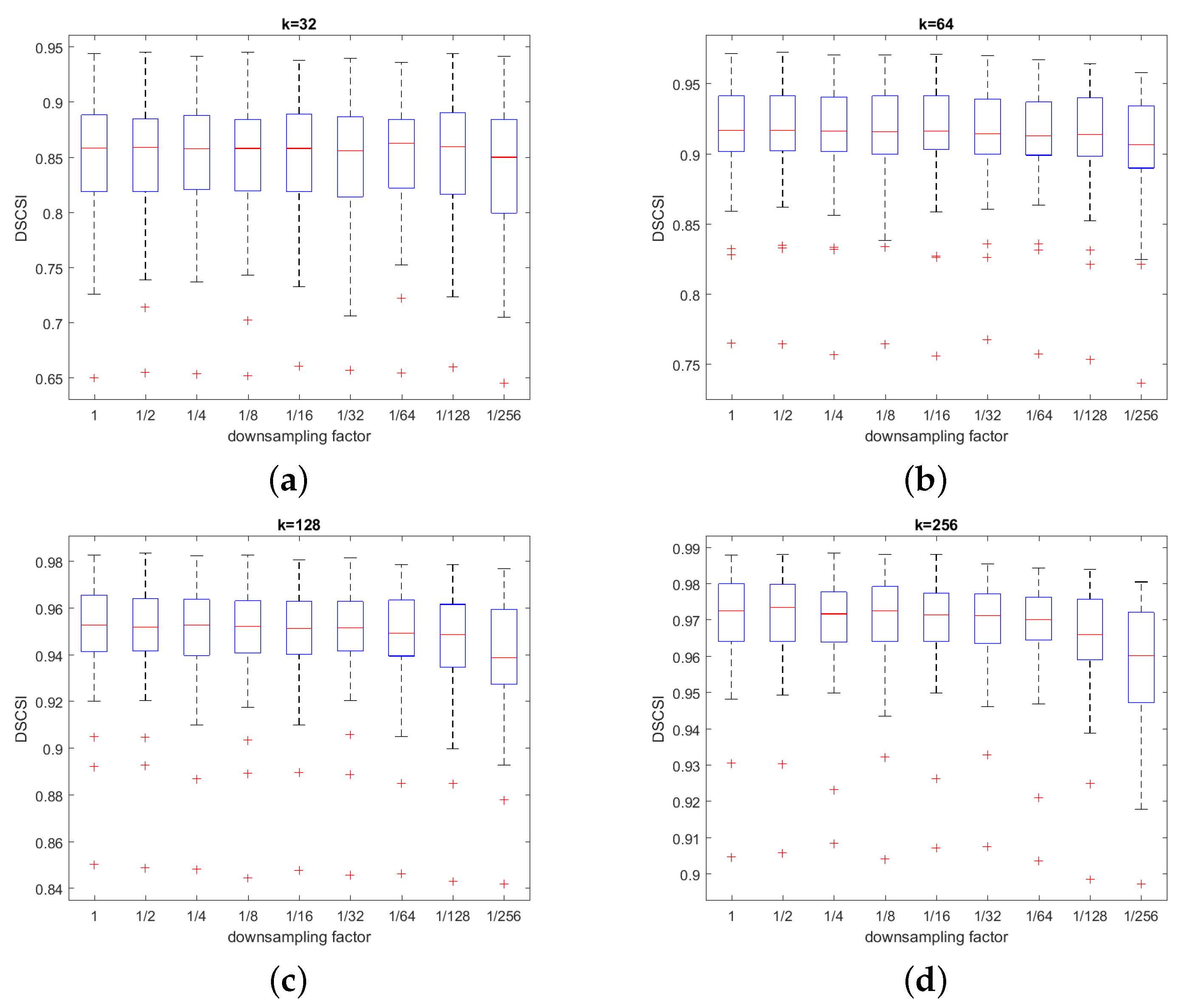
Figure 7, Figure 8 and Figure 9 show the box plots obtained for all images from the Kodak image dataset. In Figure 7, these are plots for the classic MSE quality index, while Figure 8 and Figure 9 contain quality assessments obtained for two new indices: DSCSI and HPSI. As can be seen, the decrease in image quality associated with sampling up to 1/128 is small and the change in quantization time is significant as shown in

Table 9. CPU times (in milliseconds) for the Kodak image dataset.

$\mathit{d}\mathit{f}$	k
	32	64	128	256
1	361	650	1465	2500
1/2	161	366	643	1106
1/4	80	177	347	565
1/8	46	76	165	298
1/16	22	44	75	134
1/32	11	21	37	68
1/64	6	11	19	32
1/128	3	5	7	15
1/256	2	3	4	7

. This situation occurs for all three indices of image quality.

The maximal speedup obtained in color quantization of 24 images was equal to 357 in the case of downsampling factor equal to 1/256 and a palette of 256 colors. In this case, however, the values of the quality indices deteriorated noticeably. On the other hand, such quality dropping was not observed for the case of the downsampling factor equal to 1/128, where the maximal speedup was equal to 166.

The final stage of research on the Kodak image dataset was concerned with input images of different resolutions: standard and high. In the case of high resolution images, there was no noticeable decrease in image quality due to the reduction of the downsampling factor to the value 1/256 (Figure 10).

5. Conclusions

Color quantization is still one of the important image operations. Hence, it is of great significance to design a fast color quantization method generating high quality quantized images. Such images are the result of the KM method with deterministic initialization by means of Wu’s algorithm. Unfortunately, this is not a fast method. In this paper, we introduced an improved method, which significantly accelerated the quantization (sometimes a few hundred times) while not significantly lowering the quality of the obtained image. It should be noted that not only the classic MSE index was used to assess the quantized image, but also the DSCSI and HPSI indices strongly related to the observer’s visual perception. The improvement of the method’s operation consisted in the application downsampling of the input image through the NNI. The article shows that, the higher the spatial resolution of the image, the smaller the dependence of the result obtained by the improved method on the number of colors in the palette. In the future, we will analyze the usefulness of our method to other even more time-consuming clustering-based quantization techniques such as Fuzzy C-Means (FCM), K-Harmonic Means (KHM), etc.