Application of the Symmetric Model to the Design Optimization of Fan Outlet Grills


Abstract
1. Introduction
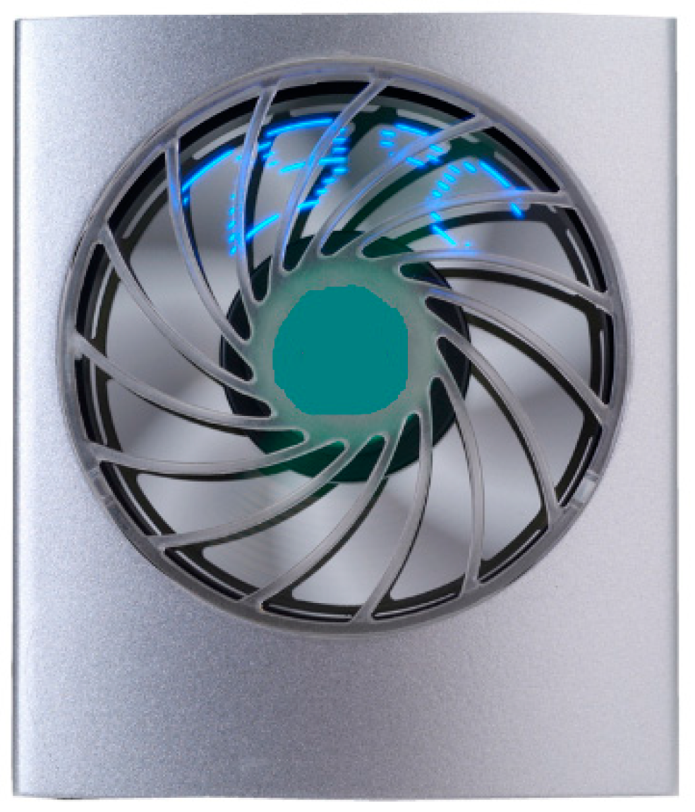
2. Research Model
Configuration of Model Parameters
3. Research Methodology
3.1. Numerical Analysis
3.1.1. Governing Equations
3.1.2. Theory of Turbulence Model
3.1.3. Standard k–ε Turbulence Model
3.1.4. RNG k−ε Turbulence Model
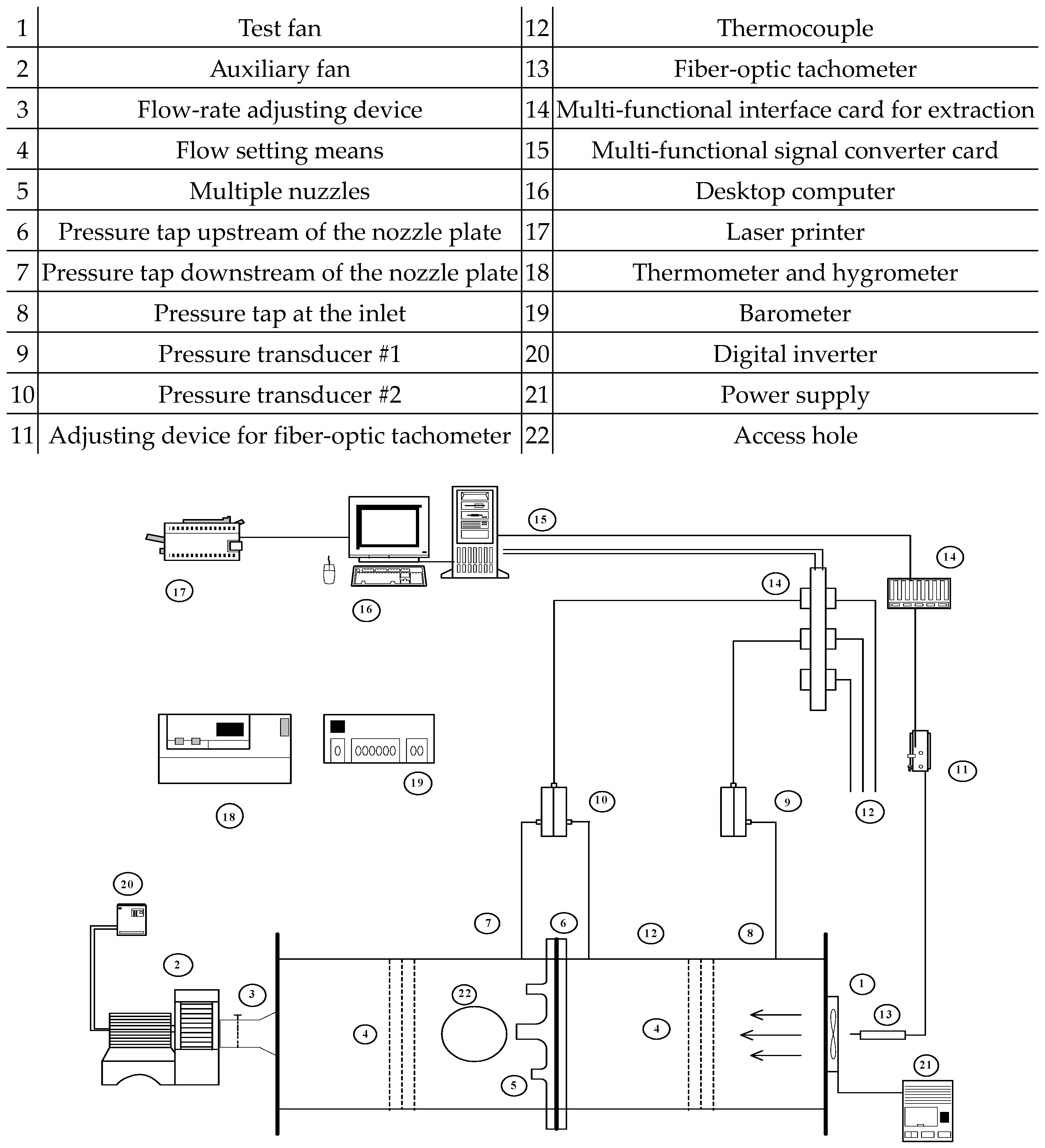
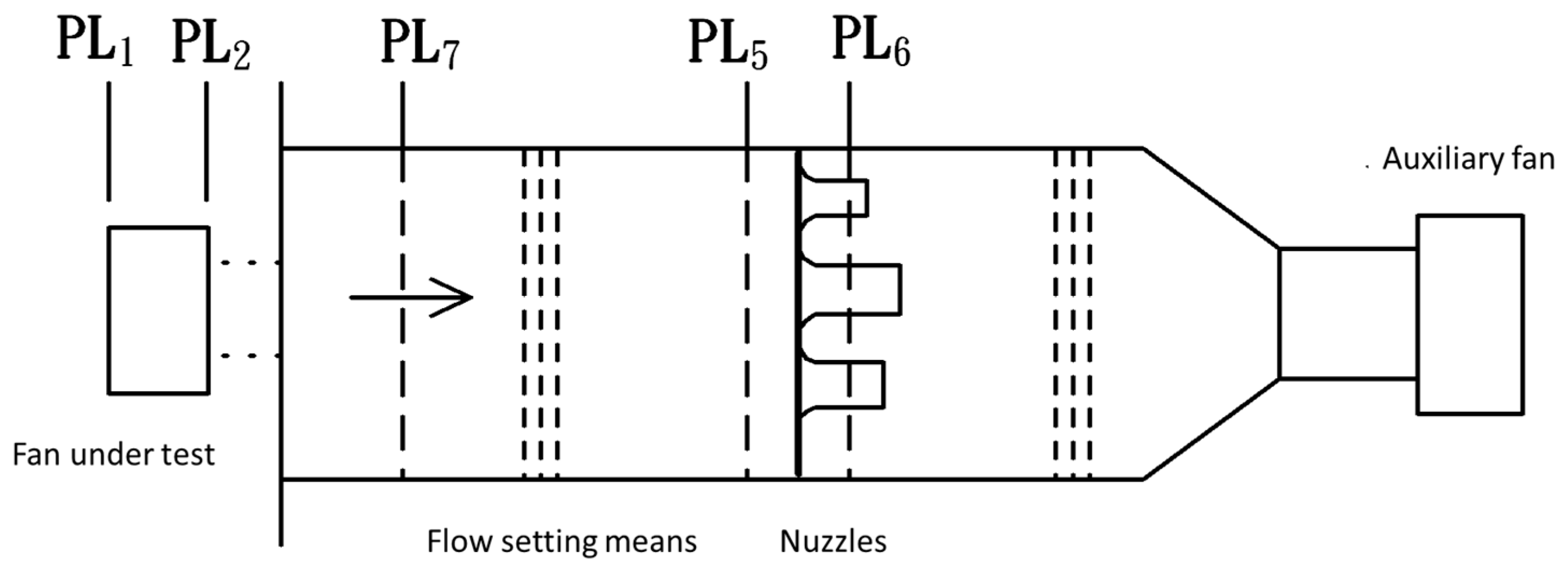
3.2. Performance Testing Equipment for Fans
3.2.1. Calculation of Flow Rates
3.2.2. Calculation of Air Pressures
3.2.3. Fan Performance Power and Efficiency
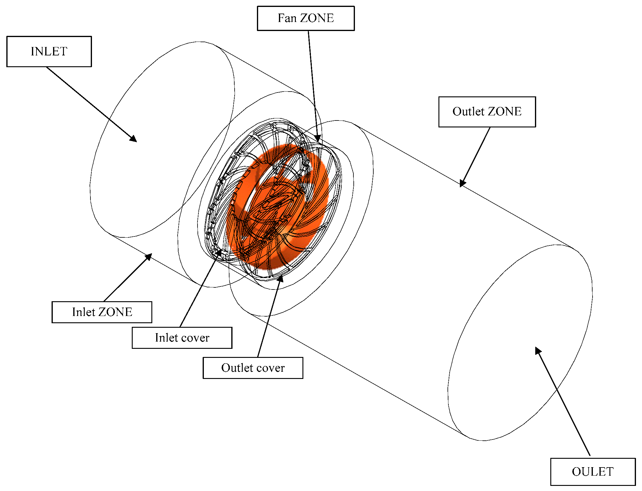
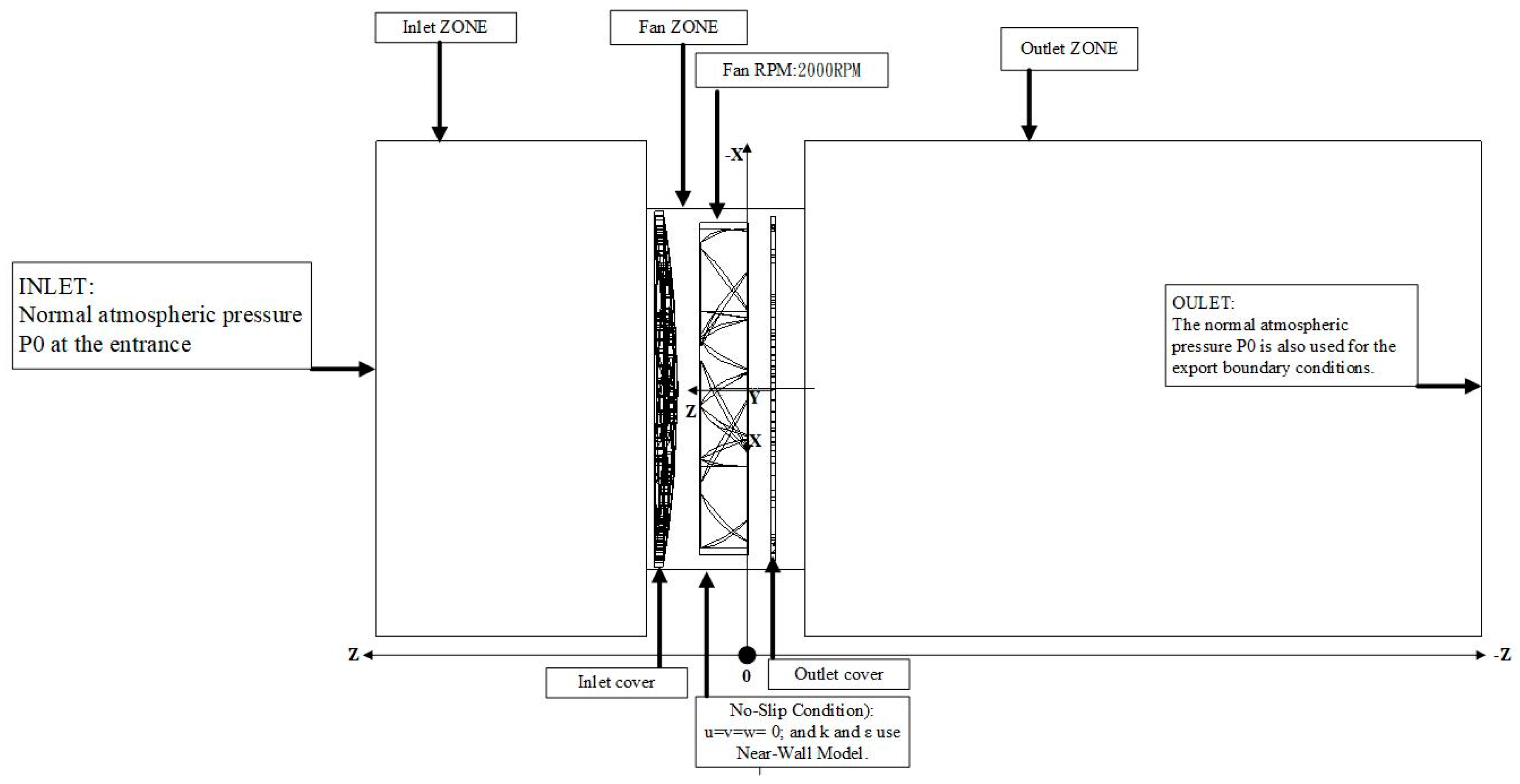
4. Numerical Simulation
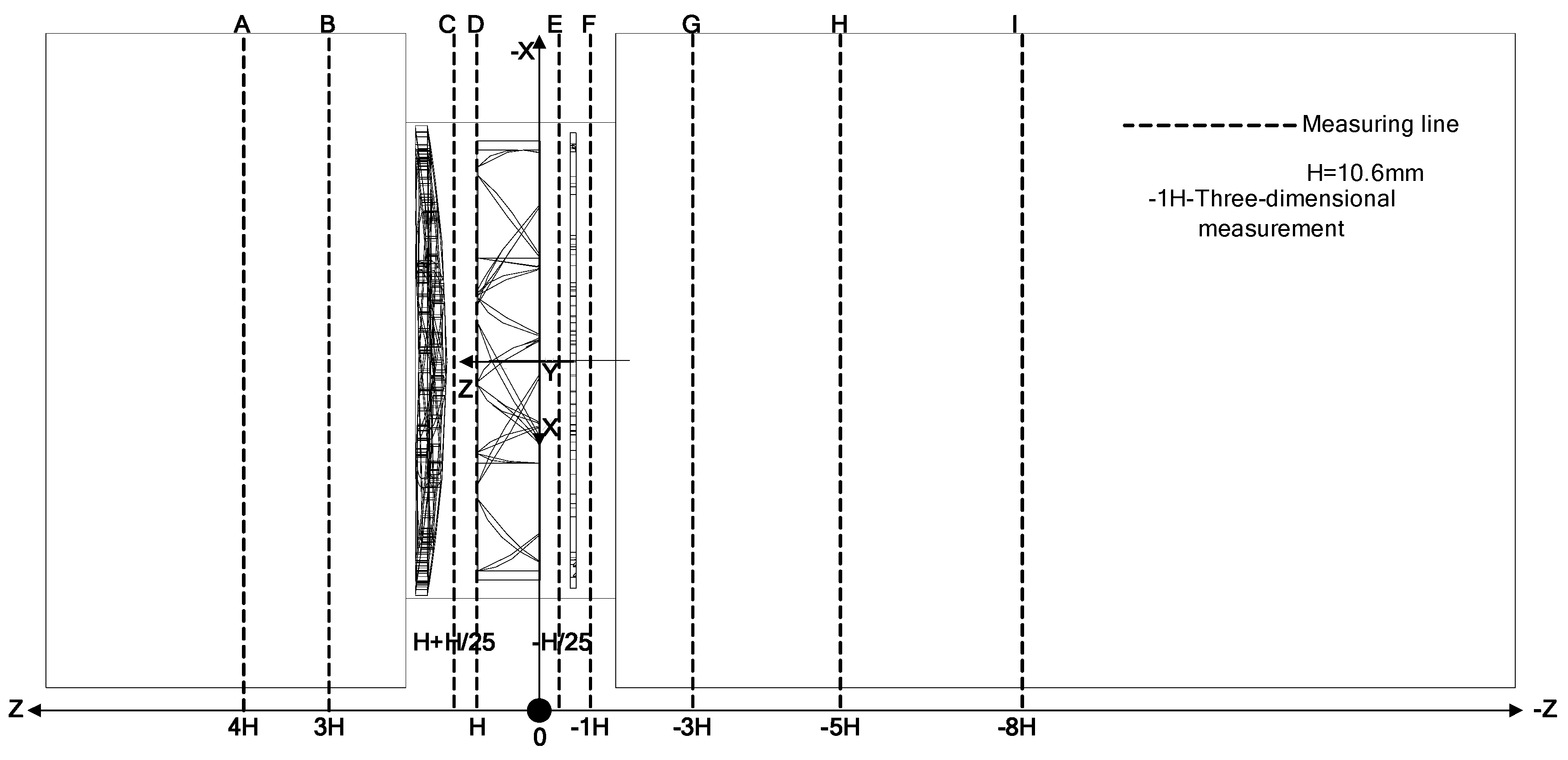
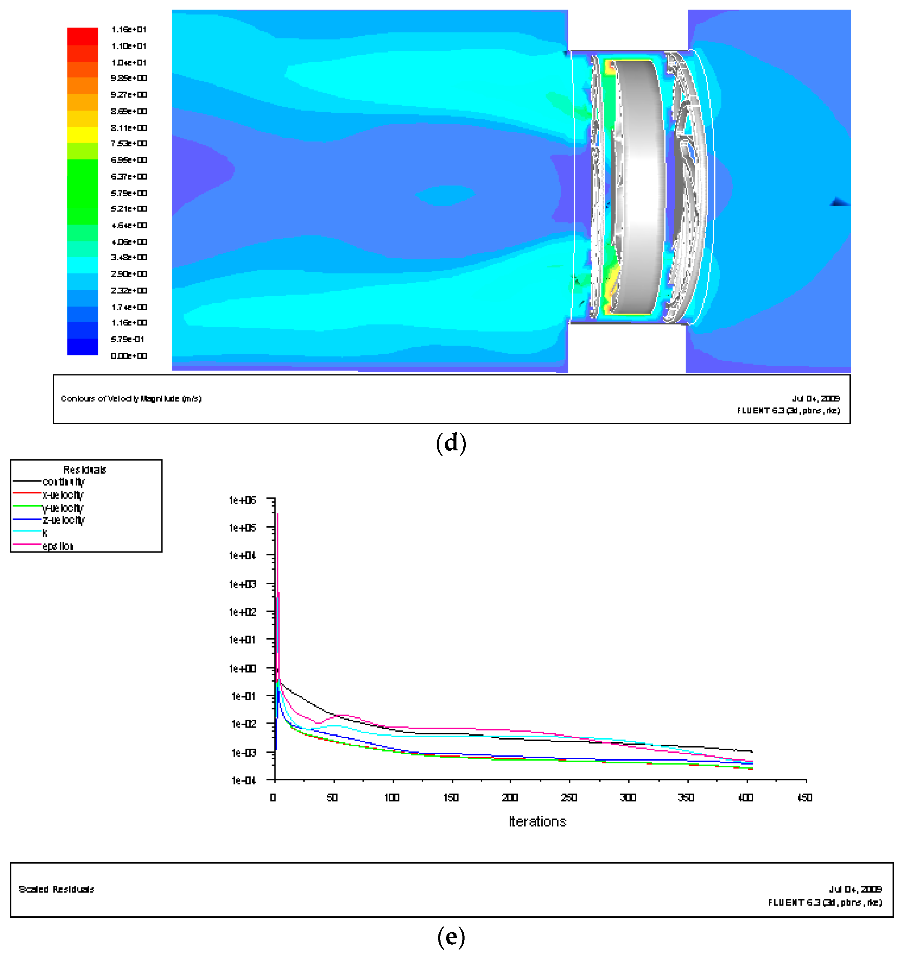
5. Verification of the Case Study and Numerical Analysis
5.1. Verification between Numerical Simulation and Experiment Testing
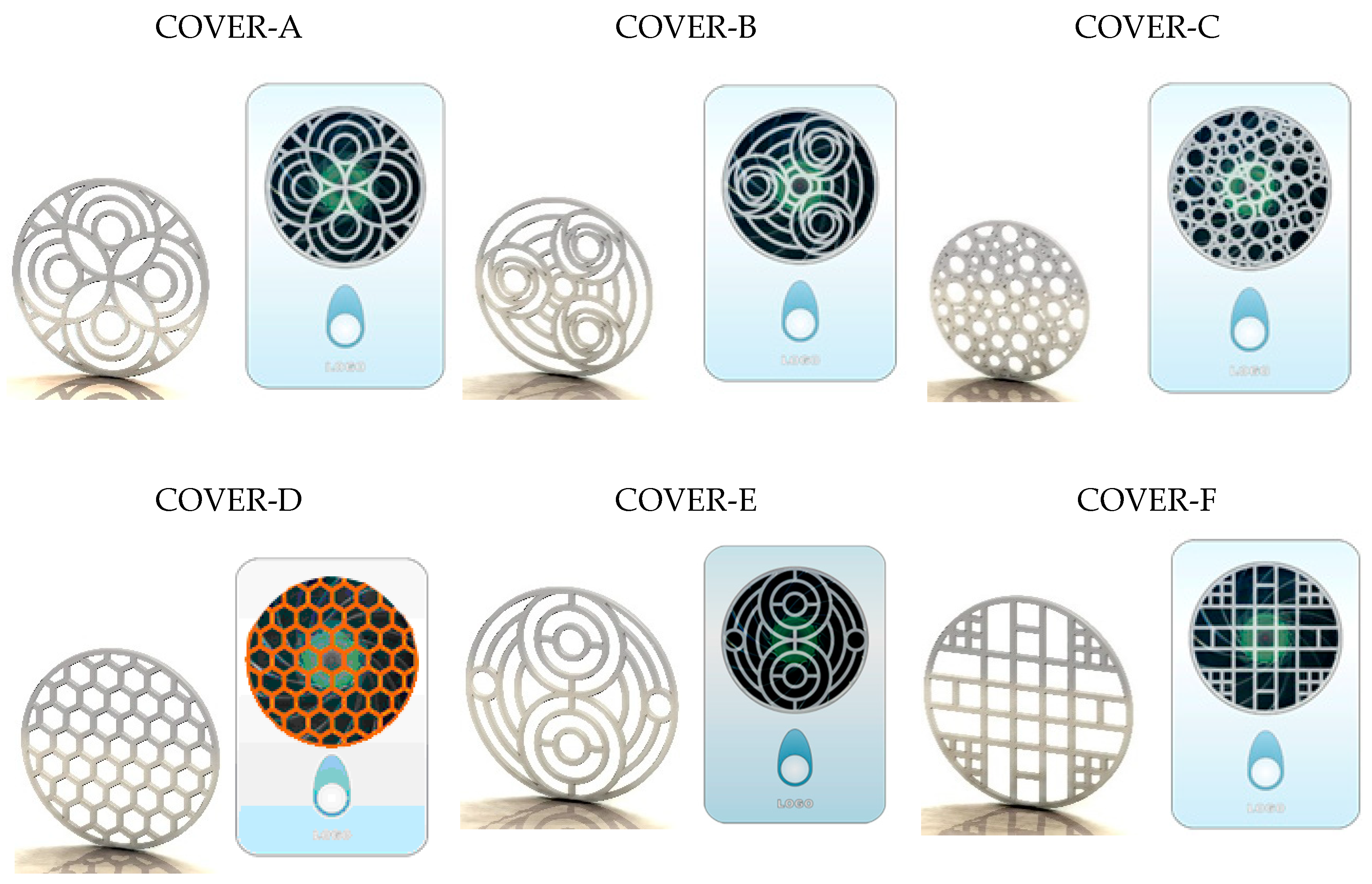
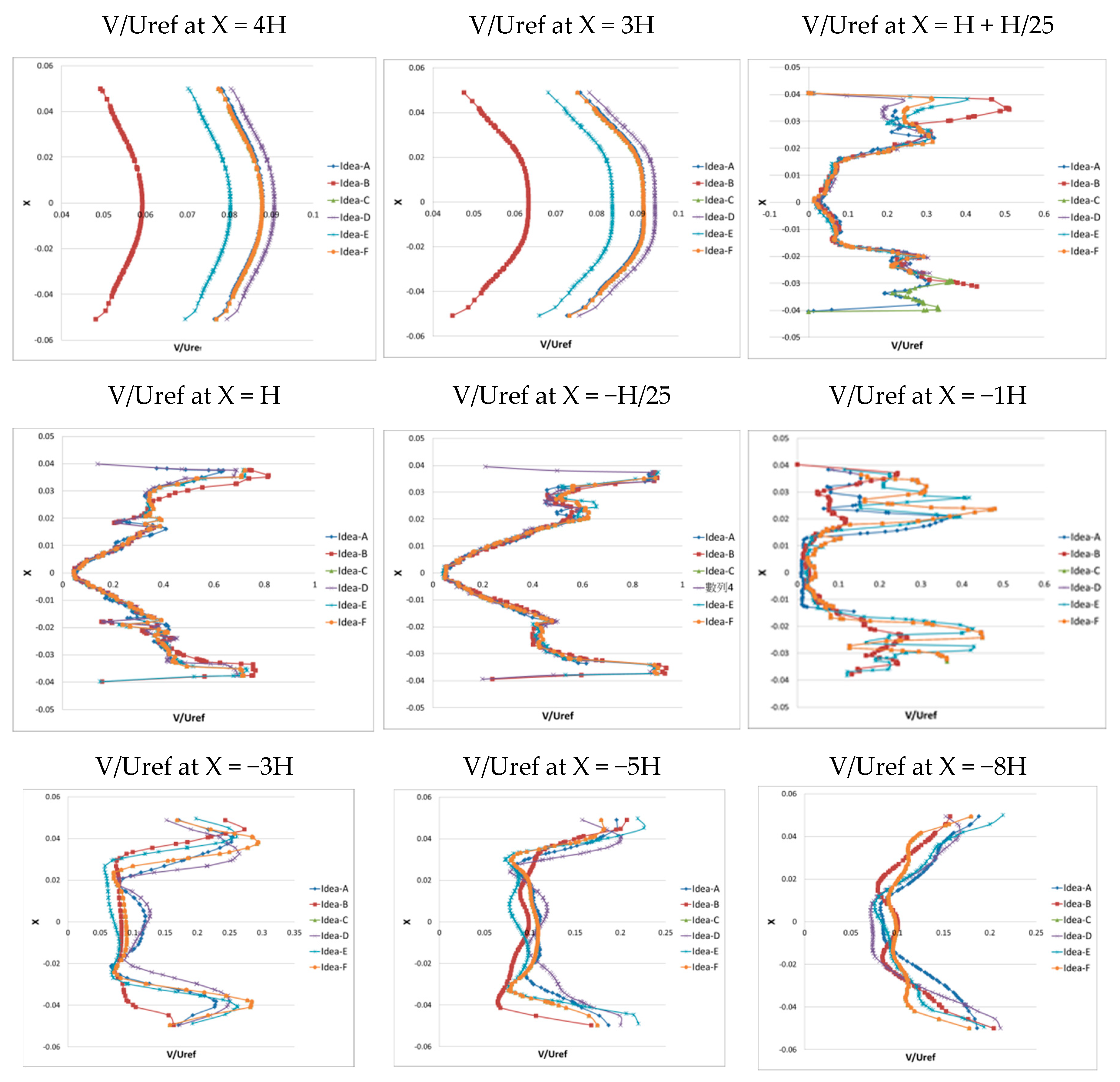
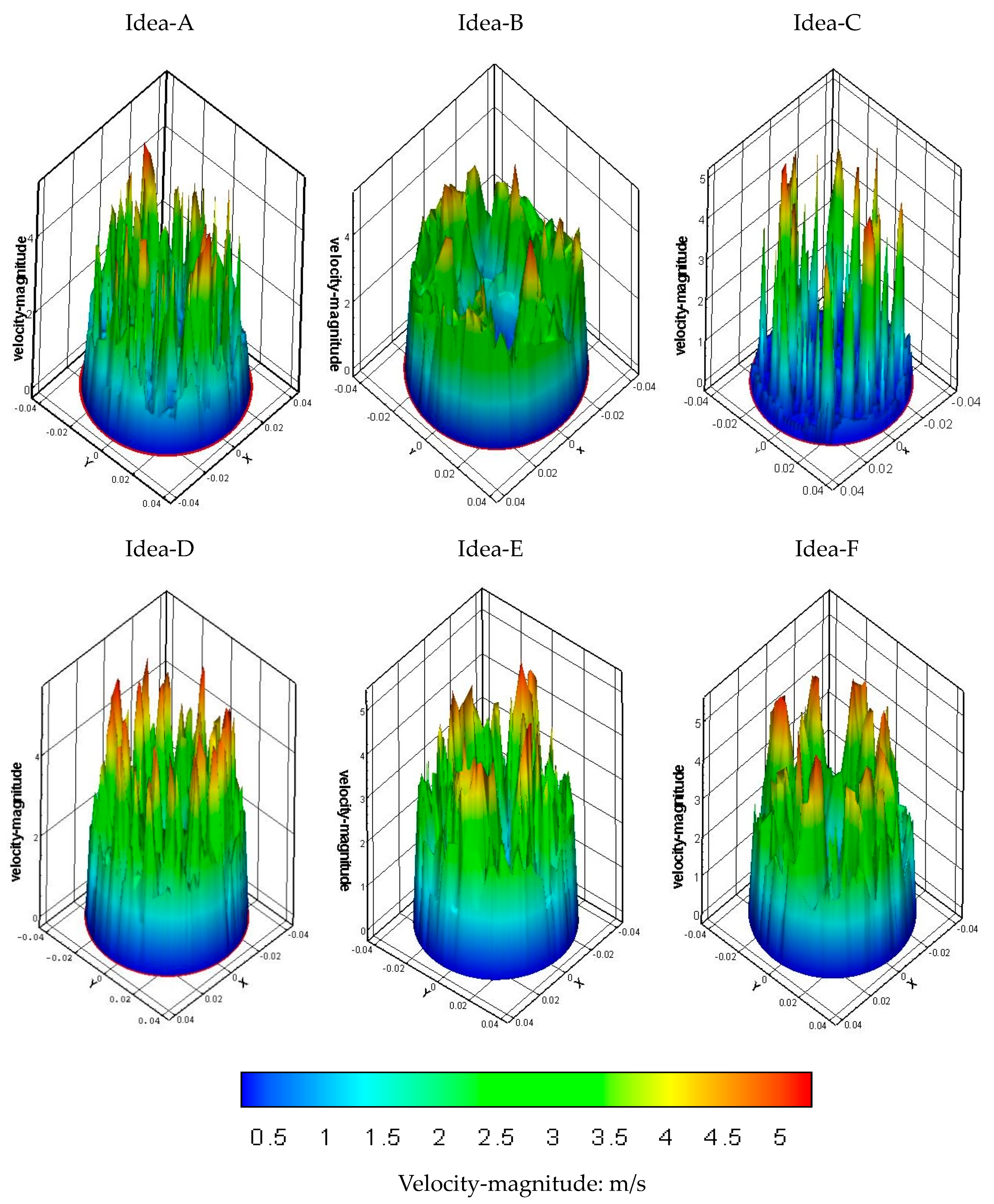
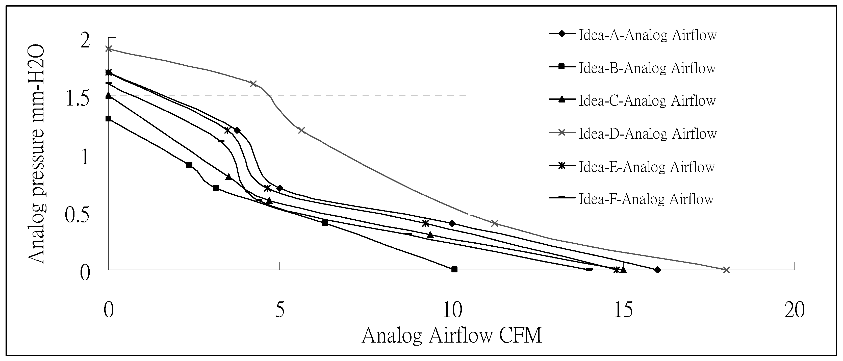
5.2. Design Cases and Comparison between Simulation Results
6. Conclusions
- The distribution at the inlet can be smoother.
- After passing through the inlet, the air pressure will increase at some portions about 1/2 of the impeller height.
- The maximum velocity at each cross-sectional plane occurs closer to the outlet.
- The change in the outlet location makes the air velocity increase and move toward the outlet direction.
- At the outlet plane of Idea-B, C, and E, many regions were found to have a low air velocity and recirculation. This phenomenon indicates inferior outlet conditions.
- Idea-D, with the honeycomb shape, had the most uniform air velocity among the six opening patterns. From the aspect of the leaving flow rate, it was also the most optimal opening pattern.
- If a fan is not improved by the airfoil design, the assessment can be carried out on the design factors of the outlet pattern.
Author Contributions
Funding
Conflicts of Interest
References
- Marinetti, S.; Cavazzini, G.; Fedele, L.; De Zan, F.; Schiesaro, P. Air velocity distribution analysis in the air duct of a display cabinet by PIV technique. Int. J. Refrig. 2012, 35, 2321–2331. [Google Scholar] [CrossRef]
- Gebrehiwot, M.G.; De Baerdemaeker, J.; Baelmans, M. Effect of a cross-flow opening on the performance of a centrifugal fan in a combine harvester: Computational and experimental study. Biosyst. Eng. 2010, 105, 247–256. [Google Scholar] [CrossRef]
- Chen, F.; Li, S.; Su, J.; Wang, Z. Experimental Study of Bowed-twisted Stators in an Axial Transonic Fan Stage. Chin. J. Aeronaut. 2009, 22, 364–370. [Google Scholar]
- Betta, V.; Cascetta, F.; Musto, M.; Rotondo, G. Fluid dynamic performances of traditional and alternative jet fans in tunnel longitudinal ventilation systems. Tunn. Undergr. Space Technol. 2010, 25, 415–422. [Google Scholar] [CrossRef]
- Li, Y.; Liu, J.; Ouyang, H.; Du, Z.-H. Internal flow Mechanism and Experimental Research of low Pressure Axial fan with Forward-Skewed Blades. J. Hydrodyn. 2008, 20, 299–305. [Google Scholar] [CrossRef]
- Delele, M.; De Moor, A.; Sonck, B.; Ramon, H.; Nicolaï, B.; Verboven, P. Modelling and Validation of the Air Flow generated by a Cross Flow Air Sprayer as affected by Travel Speed and Fan Speed. Biosyst. Eng. 2005, 92, 165–174. [Google Scholar] [CrossRef]
- Gebrehiwot, M.G.; De Baerdemaeker, J.; Baelmans, M. Numerical and experimental study of a cross-flow fan for combine cleaning shoes. Biosyst. Eng. 2010, 106, 448–457. [Google Scholar] [CrossRef]
- Chunxi, L.; Ling, W.S.; Yakui, J. The performance of a centrifugal fan with enlarged impeller. Energy Convers. Manag. 2011, 52, 2902–2910. [Google Scholar] [CrossRef]
- Stafford, J.; Walsh, E.; Egan, V. The effect of global cross flows on the flow field and local heat transfer performance of miniature centrifugal fans. Int. J. Heat Mass Transf. 2012, 55, 1970–1985. [Google Scholar] [CrossRef]
- Liu, S.H.; Huang, R.F.; Lin, C.A. Computational and experimental investigations of performance curve of an axial flow fan using downstream flow resistance method. Exp. Therm. Fluid Sci. 2010, 34, 827–837. [Google Scholar] [CrossRef]
- Zhao, X.; Sun, J.; Zhang, Z. Prediction and measurement of axial flow fan aerodynamic and aeroacoustic performance in a split-type air-conditioner outdoor unit. Int. J. Refrig. 2013, 36, 1098–1108. [Google Scholar] [CrossRef]
- Hu, B.-B.; Ouyang, H.; Wu, Y.-D.; Jin, G.-Y.; Qiang, X.-Q.; Du, Z.-H. Numerical prediction of the interaction noise radiated from an axial fan. Appl. Acoust. 2013, 74, 544–552. [Google Scholar] [CrossRef]
- Owen, M.; Kröger, D.G. Contributors to increased fan inlet temperature at an air-cooled steam condenser. Appl. Ther. Eng. 2013, 50, 1149–1156. [Google Scholar] [CrossRef]
- Moonen, P.; Blocken, B.; Roels, S.; Carmeliet, J. Numerical modeling of the flow conditions in a closed-circuit low-speed wind tunnel. J. Wind Eng. Ind. Aerodyn. 2006, 94, 699–723. [Google Scholar] [CrossRef]
- Carolus, T.; Schneider, M.; Reese, H. Axial flow fan broad-band noise and prediction. J. Sound Vib. 2007, 300, 50–70. [Google Scholar] [CrossRef]
- Bredell, J.; Kröger, D.; Thiart, G. Numerical investigation of fan performance in a forced draft air-cooled steam condenser. Appl. Eng. 2006, 26, 846–852. [Google Scholar] [CrossRef]
- Hsiao, S.-W.; Lin, H.-H.; Lo, C.-H. A study of thermal comfort enhancement by the optimization of airflow induced by a ceiling fan. J. Interdiscip. Math. 2016, 19, 859–891. [Google Scholar] [CrossRef]
- Hsiao, S.W.; Lin, H.H.; Lo, C.H.; Ko, Y.C. Automobile shape formation and simulation by a computer-aided systematic method. Concurr. Eng. Res. Appl. 2016, 24, 290–301. [Google Scholar] [CrossRef]
- Lin, H.H.; Huang, Y.Y. Application of ergonomics to the design of suction fans. In Proceedings of the 1st IEEE International Conference on Knowledge Innovation and Invention, Jeju Island, South Korea, 23–27 July 2018; pp. 203–206. [Google Scholar]
- Andrea, T. On the theoretical link between design parameters and performance in cross-flow fans. A numerical and experimental study. Comput. Fluids 2005, 34, 49–66. [Google Scholar]
- Hurault, J.; Kouidri, S.; Bakir, F. Experimental investigations on the wall pressure measurement on the blade of axial flow fans. Exp. Fluid Sci. 2012, 40, 29–37. [Google Scholar] [CrossRef]
- Lin, H.H.; Hsiao, S.W. A Study of the Evaluation of Products by Industrial Design Students. Eurasia J. Math. Sci. Technol. Educ. 2018, 14, 239–254. [Google Scholar] [CrossRef]
- Shih, Y.-C.; Hou, H.-C.; Chiang, H. On similitude of the cross flow fan in a split-type air-conditioner. Appl. Eng. 2008, 28, 1853–1864. [Google Scholar] [CrossRef]
- Kim, J.-H.; Hur, N.; Kim, W. Development of algorithm based on the coupling method with CFD and motor test results to predict performance and efficiency of a fuel cell air fan. Renew. Energy 2012, 42, 157–162. [Google Scholar] [CrossRef]
- Jason, S.; Walsh, E.; Egan, V.; Grimes, R. Flat plate heat transfer with impinging axial fan flows. Int. J. Heat Mass Transfer. 2010, 53, 5629–5638. [Google Scholar]
- Greenblatt, D.; Avraham, T.; Golan, M. Computer fan performance enhancement via acoustic perturbations. Int. J. Heat Fluid Flow 2012, 34, 28–35. [Google Scholar] [CrossRef]
- Lin, H.-H. Improvement of Human Thermal Comfort by Optimizing the Airflow Induced by a Ceiling Fan. Sustainability 2019, 11, 3370. [Google Scholar] [CrossRef]
- Lin, S.-C.; Tsai, M.-L. An integrated performance analysis for a backward-inclined centrifugal fan. Comput. Fluids 2012, 56, 24–38. [Google Scholar] [CrossRef]
- Stinnes, W.H. Effect of cross-flow on the performance of air-cooled heat exchanger fans. Appl. Ther. Eng. 2002, 22, 1403–1415. [Google Scholar] [CrossRef]
- Casarsa, L.; Giannattasio, P. Experimental study of the three-dimensional flow field in cross-flow fans. Exp. Fluid Sci. 2011, 35, 948–959. [Google Scholar] [CrossRef]
- Liu, G.; Liu, M. Development of simplified in-situ fan curve measurement method using the manufacturers fan curve. Build. Environ. 2013, 48, 77–83. [Google Scholar] [CrossRef]
- Hurault, J.; Kouidri, S.; Bakir, F.; Rey, R. Experimental and numerical study of the sweep effect on three-dimensional flow downstream of axial flow fans. Flow Meas. Instrum. 2010, 21, 155–165. [Google Scholar] [CrossRef]
- Chen, T.Y.; Shu, H.T. Flow structures and heat transfer characteristics in fan flows with and without delta-wing vortex generators. Exp. Ther. Fluid Sci. 2004, 28, 273–282. [Google Scholar] [CrossRef]
- Stafford, J.; Walsh, E.; Egan, V. Local heat transfer performance and exit flow characteristics of a miniature axial fan. Int. J. Heat Fluid Flow 2010, 31, 952–960. [Google Scholar] [CrossRef]


| Airfoil Type | Airfoil Name | Blade No. | Radius of Hub | Tip of Blade | Radius of Shroud |
|---|---|---|---|---|---|
| NACA65 | NACA65-Parabolic | 7 | 8 | 36 | 40 |
| Thickness of hub | Section No. | Tip clearance | Incidence angle of the blade at the hub | Incidence angle of the blade at the tip | Blade width at the hub |
| 23.5 | 31 | 0.75 | 50 | 35 | 11 |
| Equation | ψ |
|---|---|
| Continuity | 1 |
| X-momentum | u |
| Y-momentum | v |
| Z-momentum | w |
| Energy | I or T |
| C1ε | C2ε | Cμ | Ck | C3ε |
|---|---|---|---|---|
| 1.44 | 1.92 | 0.09 | 1.0 | 1.3 |
| Inlet boundary condition [9,32] | The inlet condition is for the initial calculation, this research simulates the fan in an infinite domain condition, therefore, at the inlet, it selects and adopts normal atmospheric pressure P0. |
| Outlet boundary condition [33] | The flow generated by the rotation of the fan is the simulated flow toward the ambient atmosphere. Therefore, the outlet boundary condition of the normal atmospheric pressure P0 is also adopted. |
| Wall boundary condition | Except for the non-permeable condition to be satisfied when a fluid flows through a wall, it also needs to satisfy the no-slip condition), i.e., u = v = w = 0. k and ε are determined by the near-wall model. |
| Assumption that is made to reduce the complexity of flow field calculation [34] | The flow field is at the steady state and the fluid is incompressible air. |
| The turbulence model is the standard k–ε model with eddy rectification. | |
| The influence of gravity is neglected. | |
| Related fluid properties such as viscosity, density, and specific heat are all constants. | |
| A rotation speed of 2000 RPM is set for the MRF fluid rotating region. | |
| The relative velocity between the solid surface and the fluid is zero, which is the no-slip condition. | |
| The influence of radiation and buoyancy is neglected. Moreover, physical properties do not vary with temperature. | |
| Rotating speed of the fan | Configured to be 2000 RPM. |
| Numerical Simulation | Experimental Result | Deviation | |
|---|---|---|---|
| Air flow rate | 16.8CFM | 16.3CFM | 3% |
| Static pressure | 1.75 mm-H2O | 1.71 mm-H2O | 2% |
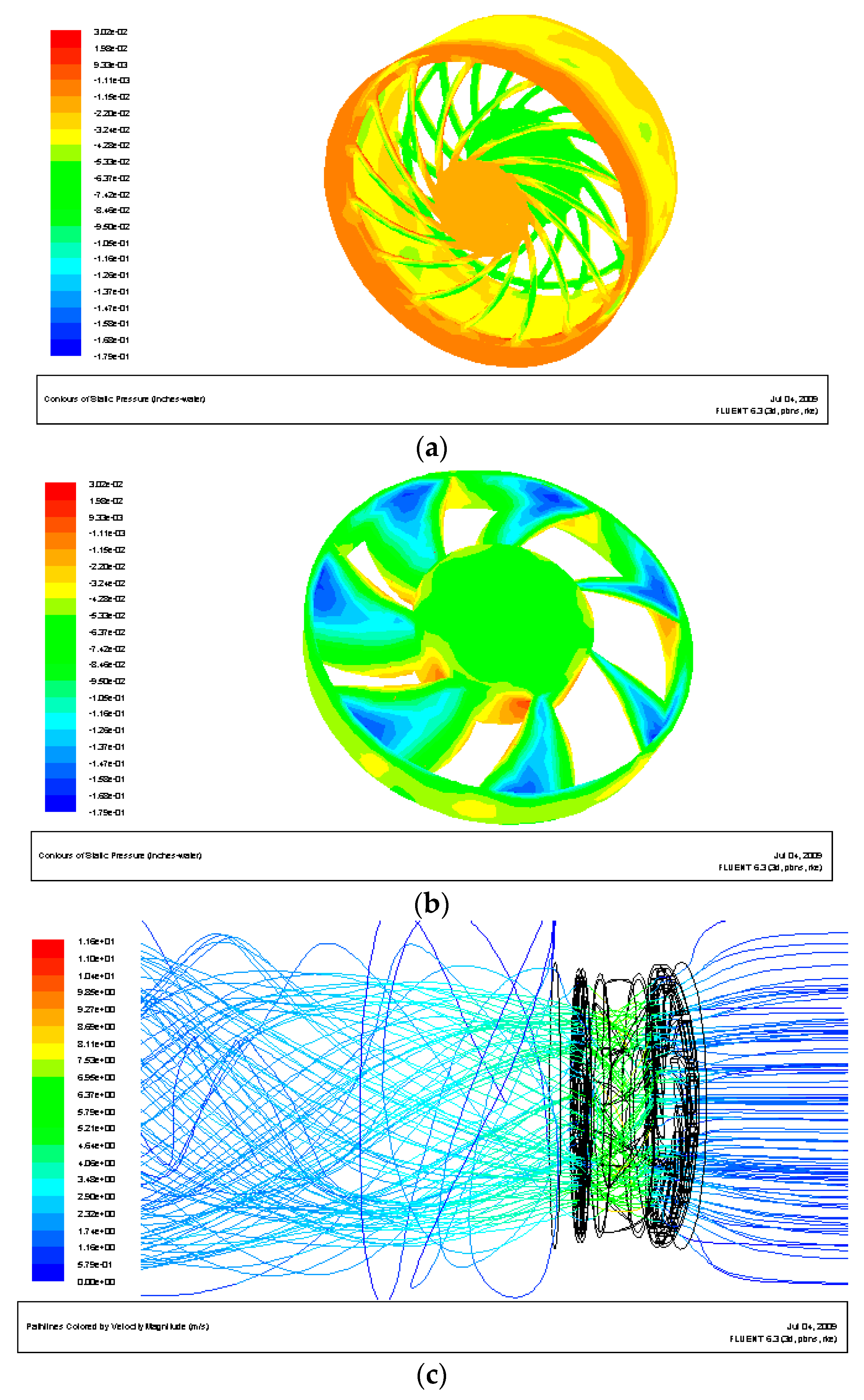
Idea-A (a) (a) | Idea-B (b) (b) | ||
 |  |  |  |
| 1(a) Pressure distribution on the fan | 1(b) Pressure distribution on the outer cover | 2(a) Pressure distribution on the fan | 2(b) Pressure distribution on the outer cover |
 |  |  |  |
| 1(c) Velocity distribution | 1(d) Streamline distribution | 2(c) Velocity distribution | 2(d) Streamline distribution |
Idea-C (c) (c) | Idea-D (d) (d) | ||
 |  |  |  |
| 3(a) Pressure distribution on the fan | 3(b) Pressure distribution on the outer cover | 4(a) Pressure distribution on the fan | 4(a) Pressure distribution on the fan |
 |  |  |  |
| 3(c) Velocity distribution | 3(d) Streamline distribution | 4(c) Velocity distribution | 4(c) Flow field distribution |
Idea-E (e) (e) | Idea-F (f) (f) | ||
 |  |  |  |
| 5(a) Pressure distribution on the fan | 5(b) Pressure distribution on the outer cover | 6(a) Pressure distribution on the fan | 6(b) Pressure distribution on the outer cover |
 |  |  |  |
| 5(c) Velocity distribution | 5(d) Streamline distribution | 6(c) Velocity distribution | 6(d) Streamline distribution |
© 2019 by the authors. Licensee MDPI, Basel, Switzerland. This article is an open access article distributed under the terms and conditions of the Creative Commons Attribution (CC BY) license (http://creativecommons.org/licenses/by/4.0/).
Share and Cite
Lin, H.-H.; Cheng, J.-H. Application of the Symmetric Model to the Design Optimization of Fan Outlet Grills. Symmetry 2019, 11, 959. https://doi.org/10.3390/sym11080959
Lin H-H, Cheng J-H. Application of the Symmetric Model to the Design Optimization of Fan Outlet Grills. Symmetry. 2019; 11(8):959. https://doi.org/10.3390/sym11080959
Chicago/Turabian StyleLin, Hsin-Hung, and Jui-Hung Cheng. 2019. "Application of the Symmetric Model to the Design Optimization of Fan Outlet Grills" Symmetry 11, no. 8: 959. https://doi.org/10.3390/sym11080959
APA StyleLin, H.-H., & Cheng, J.-H. (2019). Application of the Symmetric Model to the Design Optimization of Fan Outlet Grills. Symmetry, 11(8), 959. https://doi.org/10.3390/sym11080959