Article

Improved Chaotic Particle Swarm Optimization Algorithm with More Symmetric Distribution for Numerical Function Optimization

School of Mechanical, Electrical & Information Engineering, Shandong University, Weihai 264209, China
*
Author to whom correspondence should be addressed.
Symmetry 2019, 11(7), 876; https://doi.org/10.3390/sym11070876
Submission received: 4 June 2019 / Revised: 30 June 2019 / Accepted: 3 July 2019 / Published: 3 July 2019

Abstract

:
As a global-optimized and naturally inspired algorithm, particle swarm optimization (PSO) is characterized by its high quality and easy application in practical optimization problems. However, PSO has some obvious drawbacks, such as early convergence and slow convergence speed. Therefore, we introduced some appropriate improvements to PSO and proposed a novel chaotic PSO variant with arctangent acceleration coefficient (CPSO-AT). A total of 10 numerical optimization functions were employed to test the performance of the proposed CPSO-AT algorithm. Extensive contrast experiments were conducted to verify the effectiveness of the proposed methodology. The experimental results showed that the proposed CPSO-AT algorithm converges quickly and has better stability in numerical optimization problems compared with other PSO variants and other kinds of well-known optimal algorithms.

1. Introduction

With the development of artificial intelligence and the increasing computational demands of industrial design stimulated by continuously developing industry, various optimization algorithms have been increasingly studied and applied in academia and industry. Optimization algorithms are more often being applied to real-world problems, such as artificial intelligence [1], logic circuit design [2], and system identification [3].
If traditional technology is adopted to solve problems in actual optimization tasks, time would be wasted and finding the solution would be difficult. Therefore, it was essential to develop new optimization algorithms. In the past 20 years, scholars and industry specialists have presented many natural heuristic algorithms, like particle swarm optimization (PSO) [4,5], sine cosine algorithm (SCA) [6], ant colony optimization (ACO) [7], biogeography-based optimization (BBO) [8], grey wolf optimizer (GWO) [9], differential evolution (DE) [10], krill herd (KH) algorithm [11], moth flame optimization (MFO) [12], and the whale optimization algorithm (WOA) [13]. These intelligent algorithms are well-known examples.
As a nature-inspired method, PSO can simulate the social behavior of individuals in fish or bird populations. This method is not only efficient and robust but can also be easily implemented with any computer language [14,15,16]. Therefore, the industry has already adopted this algorithm to search for the best solutions to stated problems. Researchers compared the performance of PSO with other similar and population-based heuristic optimum techniques (e.g., artificial bee colony (ABC) [17], differential evolution (DE) algorithm [18] and ant lion optimizer (ALO) [19]) and found that the results obtained by PSO were generally better.
How to design a testing method that can provide a fair and objective evaluation of different kinds of optimization algorithms is an interesting and meaningful topic. It is generally known that for deterministic optimization algorithms, rigorous theoretical proof of convergence is essential and important, while for heuristic optimization algorithms, it is very hard to prove convergence theoretically, therefore researchers in this field usually conduct extensive experiments to verify the effectiveness of the proposed methodology [20,21]. Hooker, a pioneer in the integration of optimization and constraint programming technologies, discussed the drawbacks of competitive testing and the benefits of scientific testing [22]. In [23], Sergeyev et al. proposed a new visual technique for a systematic comparison of global optimization algorithms having different natures. The proposed operational zones and aggregated operational zones are powerful tools for reliable comparison of deterministic and stochastic global optimization algorithms. This new testing methodology is a promising method that can be widely applied by researchers from optimization fields in the near future.
The PSO algorithm is simple and efficient, and is widely applied in practical engineering for global optimization. However, in [24], the authors conducted many theoretical derivations and simulation experiments to discuss the performance of global random search algorithms for large dimensions, and they concluded that if the dimension of the feasible domain was large then it was virtually impossible to guarantee that the global minimizer was reached by a general global random search algorithm. Therefore, according to the above conclusion, PSO and its variants are not suitable for solving complex high-dimensional optimization problems theoretically. In addition, PSO has some other shortcomings such as a premature and slow convergence speed. To overcome these deficiencies, many researchers have introduced different methods to enhance the performance of PSO. Compared with the basic PSO, these well-designed PSO variants not only have excellent convergence speed, but also have a strong global optimization ability. However, for special circumstances, such as solving complex optimization problems with different test functions, the robustness, population diversity and the ability to balance local exploitation and global exploration is still insufficient.

2. Review of Previous Work

Particle Swarm Optimizer

Eberhart and Kennedy proposed the PSO algorithm, which is an evolutionary computational technique invented from the study of the predation behavior of bird flocks. The location of each particle represents a candidate solution, and the fitness of the solution depends on the fitness function. In each iteration, the particles update their speed and position by dynamically tracking the two extremes including the individual best solution ( p b e s t i ) found by the individual and the global final value ( g b e s t ) currently found by the entire population.
Set in D-dimensional target search space, there is a group of m particles, then the i-th particle can be represented by a D-dimensional vector, and its position can be denoted as X i = ( x i 1 , x i 2 , , x i D ) T , i = 1 , 2 , , m . The flight speed is also a D-dimensional vector that can be denoted as V i = ( v i 1 , v i 2 , , v i D ) T . The optimal position of the i-th particle searched so far is p b e s t i , and the optimal position searched by the entire particle swarm is g b e s t . The d-th dimension of the velocity and position of the i-th particle in the (t+1)-th iteration are updated as follows:
V i , d t + 1 = ω × V i , d t + c 1 × r 1 × ( p b e s t i , d t X i , d t ) + c 2 × r 2 × ( g b e s t d t X i , d t )
X i , d t + 1 = X i , d t + V i , d t + 1
where ω is the inertia weight; r 1 and r 2 are random numbers within [0,1]; c 1 and c 2 represent learning factors; c 1 r 1 ( p b e s t i d X i d ) is the individual cognition term, which represents the individual cognitive experience of the particles, and it causes the particles to move toward the best position they experience; and c 2 r 2 ( g b e s t d X i d ) is the social cognition term, which denotes the influence of the group experience on the flight path of particles. The social cognition term moves the particles toward the best position found by the group, representing the sharing of information between the particles.
Shi and Eberhart introduced a famous PSO variant with a linear decreasing inertia weight. In [25], the proposed method adds this improvement using Equation (3) to avoid premature convergence. The improved mechanism is as follows:
ω = ω max M j M max × ( ω max ω min )
where M j and M max denote the number of present iterations and the maximum number of iterations defined by the user, respectively.

3. Chaotic Particle Swarm Optimization- Arctangent Acceleration Coefficient Algorithm

Because the PSO algorithm lacks diversity in its search process [26,27,28,29], the search is prone to stagnation due to early convergence. Moreover, the PSO algorithm cannot escape from the local optimal solution efficiently and the optimization of the solution is poor. Based on in-depth research on PSO improvements, three well designed improvements were introduced to enhance the performance of the PSO.

3.1. Chaotic Particle Swarm Optimization (CPSO)

The initialization of the particle swarm is important for the convergence speed of the PSO algorithm and the quality of the solution. During the stage of particle swarm initialization, as no prior knowledge is available, the position and velocity of the particles are generally determined by random initialization. Although the random distribution of particle swarms is effective to some extent, some particles may affect the convergence speed of the algorithm because they are too far away from the optimal solution. Chaotic motion occurs in various states in the chaotic attraction domain, and does not lose the required randomness of particle group initialization.
Chaos is a relatively common phenomenon in nonlinear systems. It is characterized by ergodicity and inherent randomness and can traverse all states in a particular range according to its law. Logistic mapping is a typical chaotic system, and the mapping relationship is as follows:
z i + 1 = μ z i ( 1 z i ) , z i ( 0 , 1 ]
where μ is the control variable. When μ = 4, the logistic map is completely chaotic, and the chaotic variable z i generated at this time has better ergodicity.
Figure 1 shows the bifurcation diagram of the logistic chaotic map. The chaotic map can distribute the particle swarm to the random value in the interval [0,1] during the search. However, the traditional chaotic mapping formula in Equation (4) distributes the particles more in the area 0 and 1, as shown in Figure 1. This causes the non-uniformity of the chaotic distribution, which prevents the even distribution of the particles in the [0, 1] interval during the chaotic search process.
Based on Equation (4), we used the cosine function to optimize it, with the goal of more evenly distributing the particles in the [0, 1] interval, and the new mapping relationship was defined as follows:
z i + 1 = cos ( μ z i ( 1 z i ) ) , z i ( 0 , 1 ]
The chaos algorithm can be understood as: given an initial value, the pseudo-random sequence is generated by the initial iteration, and each iteration aims to realize a search. Through continuous iterations, the traversal search of the chaotic space can be realized. The chaotic algorithm implements a non-repetitive traversal search, thus fundamentally solving the local extreme problem in the PSO algorithm. Figure 2 illustrates the bifurcation diagram of the logistic map for Equation (5).
We propose two main ways to use the logistic chaotic algorithm:
(1)
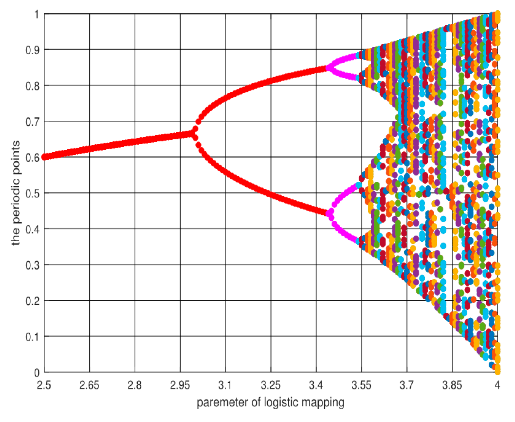
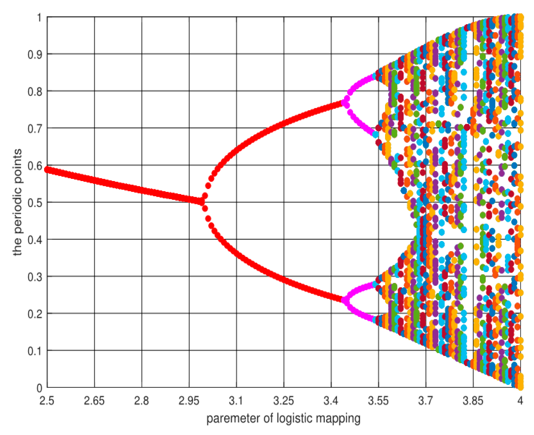
A random sequence Z between chaotic [0, 1] is generated by an iteration of an initial value between [0, 1] through the iteration of the logistic equation: a 0 , a 1 , a 2 … Through linear mapping using Equation (6), the chaos is extended to the value range of the optimization variable X [ a , b ] to achieve traversal of the range of values of the optimized variables.
Z X : X = a + ( b a ) × cos ( Z )
(2)
Generate a chaotic random sequence Z between [0, 1] using the logistic equation, and then pass the carrier map in Equation (7), introducing chaos into g b e s t , a nearby area, to achieve local chaotic search:
Z Y : X = g b e s t + R × cos ( Z )
where R is the search radius used to control the range of local chaotic search. Through experiments, we found that there was a good optimization effect when R [ 0.1 , 0.4 ] .

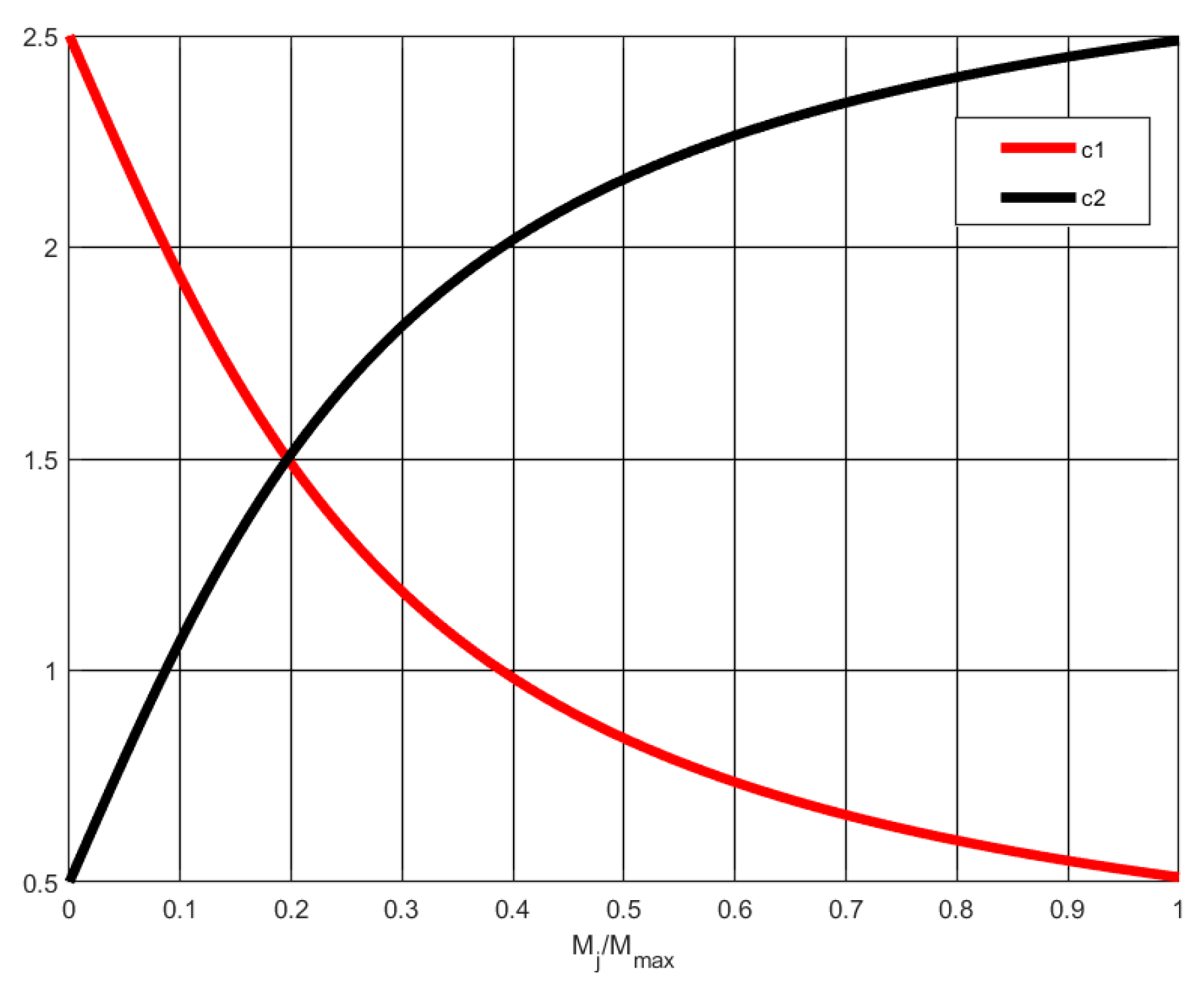
3.2. Arc Tangent Acceleration Coefficients (AT)

Using arc tangent acceleration coefficients (AT), we propose a novel cognitive and social component parameter adjustment strategy in this paper. Compared with constant values, AT has a better ability to balance the overall search during the previous period and local convergence in the later stage. In AT, the parameters c 1 and c 2 are defined by Equation (8) and Equation (9), respectively.
c 1 = × arctan ( ( M j M max ) × σ ) + δ 1
c 2 = × arctan ( ( M j M max ) × σ ) + δ 2
where and σ , and δ 1 and δ 2 are constant ( = 1.5, σ = 4, δ 1 = 2.5, and δ 2 = 0.5).
The range of values of c 1 and c 2 are illustrated in Figure 3, from which we can see c 1 ranged from 2.5 to 0.5 and c 2 ranged from 0.5 to 2.5.

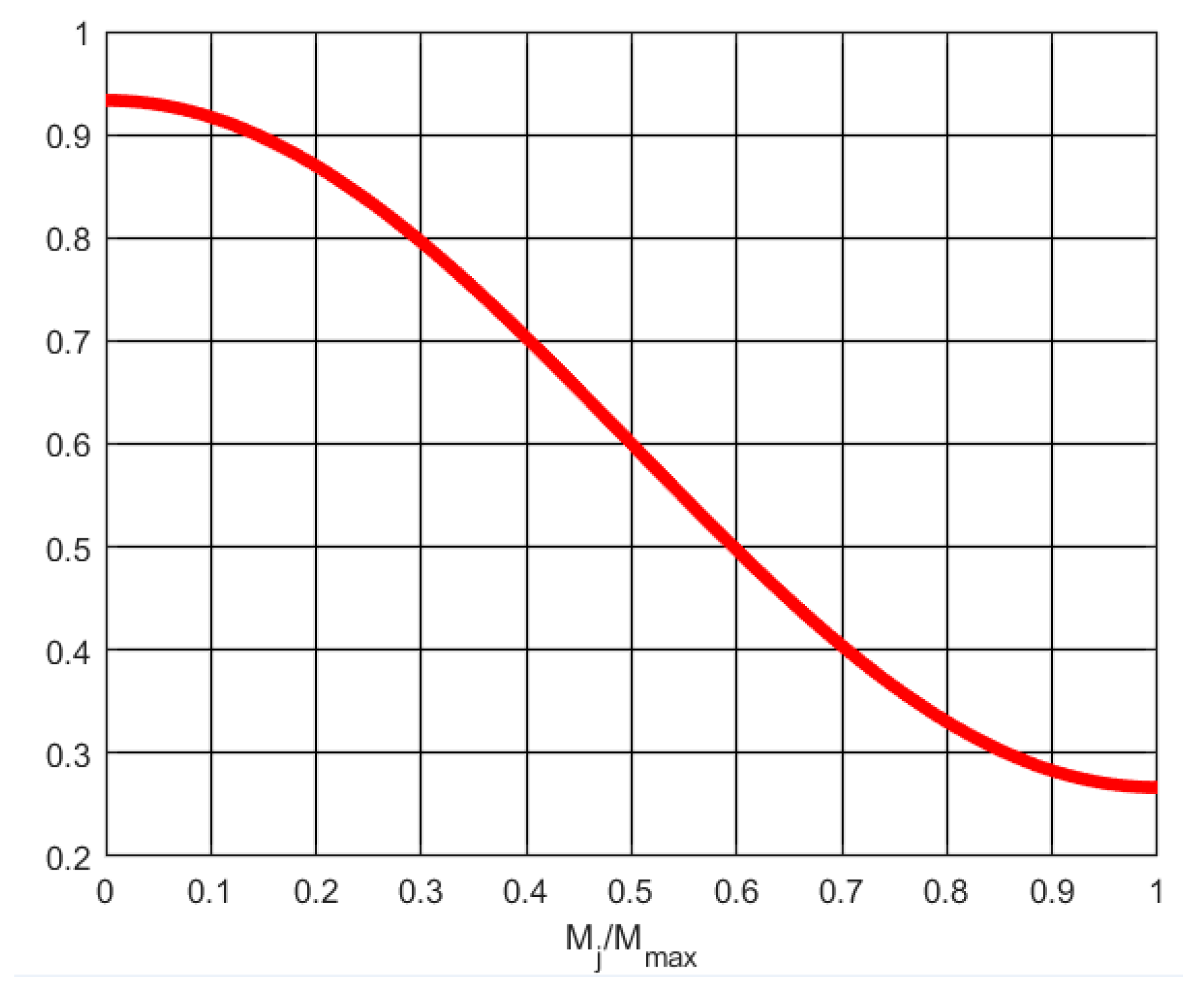
3.3. Cosine Map Inertia Weight

When the inertia weight is large, it is convenient for the global search, and when the inertia weight is small, the local search is enhanced. According to previous studies [30,31], the sine function plays an important role in adjusting ω. Inspired by this idea, we proposed an improved cosine function, which was defined by Equation (10).
ω = φ × cos ( ( M j M max ) × π ) + τ
where φ and τ are constant ( φ = 1/3, τ = 0.6)
Compared with the traditional PSO algorithm, the improved cosine function can facilitate the PSO algorithm because of its global search in the early stages and local convergence in the later period. After many comparative experiments, we found that the optimal effect was obtained when φ = 1/3, τ = 0.6. In this case, ω ranged between 0.9333 and 0.2667 and the change curve was depicted in Figure 4.
Based on the above explanation, the pseudo-code of the proposed hybrid PSO variant CPSO-AT algorithm is shown in Algorithm 1.
Algorithm 1. Pseudo-code of the Chaotic Particle Swarm Optimization—Arctangent Acceleration algorithm.
1 Initialize the parameters (PS, D, V min , V max , M max , c 1 , c 2 , X min , X max )
2 The particle swarm positions X i ( i = 1 , 2 , , P S ) are initialized by chaos theory by Equation (6)
3 Randomly generate N initial velocities within the maximum range
4 PSO algorithm is used to search for individual extremum and global optimal solutions
5 Local search:
6 While Iter < Mmax do
7  Update the inertia weight ω using Equation (10)
8  Using Equations (8) and (9) to update the cognitive component c1 and social component c2.
9for i = 1:PS (population size) do
10    The speed V i of the particle X i is updated using Equation (1)
11    Use Equation (2) to update the position of particle X i
12    Calculate the fitness values f i of the new particle X i
13    if X i is superior to p b e s t i
14     Set X i to be p b e s t i
15    End if
16    if X i is superior to g b e s t
17    Set X i to be g b e s t
18    End if
19 Global search:
20 Chaotic search K times near g b e s t
21 Use the following formula Z Y : X = g b e s t + R × cos ( Z ) (Equation (7))
22 K chaotic search points near p b e s t i are obtained
23for j=1:K do
24    if f ( X ) < f ( g b e s t )
25    Set f ( X ) to be g b e s t
26    End if
27End for
28    Iter = Iter +1
29 End While

4. Simulation Experiments, Settings and Strategies

For the basic PSO and its variants listed in Table 1, the maximum iteration steps for all functions were defined as 2000, and the population size was set to 100. For the acceleration parameters for basic PSO and classical PSO, we set c 1 = c 2 = 2.0 . The dimension values of each classic test function in Table 2 were set to 30 and 50 in turn.
Table 2 lists the 10 classical benchmark functions that were applied to verify the performance of the proposed CPSO-AT. In this paper, benchmark functions were separated into two groups. The first group contained five single-modal functions and the second group consisted of five multi-modal functions. There were many local optimizations in f 8 (Rastrigin), which caused more difficulties when searching for the global optimum. f 7 (Ackley) is famous for a rather narrow global optimal basin, which means this function has many local optimums. In Table 2, we used dim and s to represent the solution space dimension and a subset of R n , respectively. For each test function, 30 independent experiments were conducted.

5. Experimental Results and Discussion

In this study, the performance of the CPSO-AT algorithm was verified using extensive simulation experiments. These experiments can be divided into two groups. The first group compared CPSO-AT with basic PSO, classical PSO, and CPSO using 10 well-known standard test functions in 30 and 50 dimensions. The simulation results are shown in Table 3 and Table 4. The second group compared CPSO-AT with other kinds of well-known optimization algorithms (MFO, KH and BBO) using the same conditions as the first group, and the parameter settings and experimental results are presented in Table 5, Table 6 and Table 7, respectively.
The k in Table 3, Table 4, Table 6 and Table 7 is a performance indicator. When k was 0, the performance of the CPSO-AT optimization was worse than that of the other algorithms; when k was 1 (non-text bold), the CPSO-AT optimization was slightly better than the other algorithms; when k was 1 (bold), the CPSO-AT optimization was superior to the other algorithms and the effect was more obvious. In addition, the best solutions are shown in bold in Table 3, Table 4, Table 6 and Table 7.
As shown in Table 5, the parameters of MFO, KH, BBO and CPSO-AT were set as follows: the number of iterations was 2000, the population size was 50, and the comparison experiments were performed on the standard test functions (shown in Table 2) in 30 and 50 dimensions.

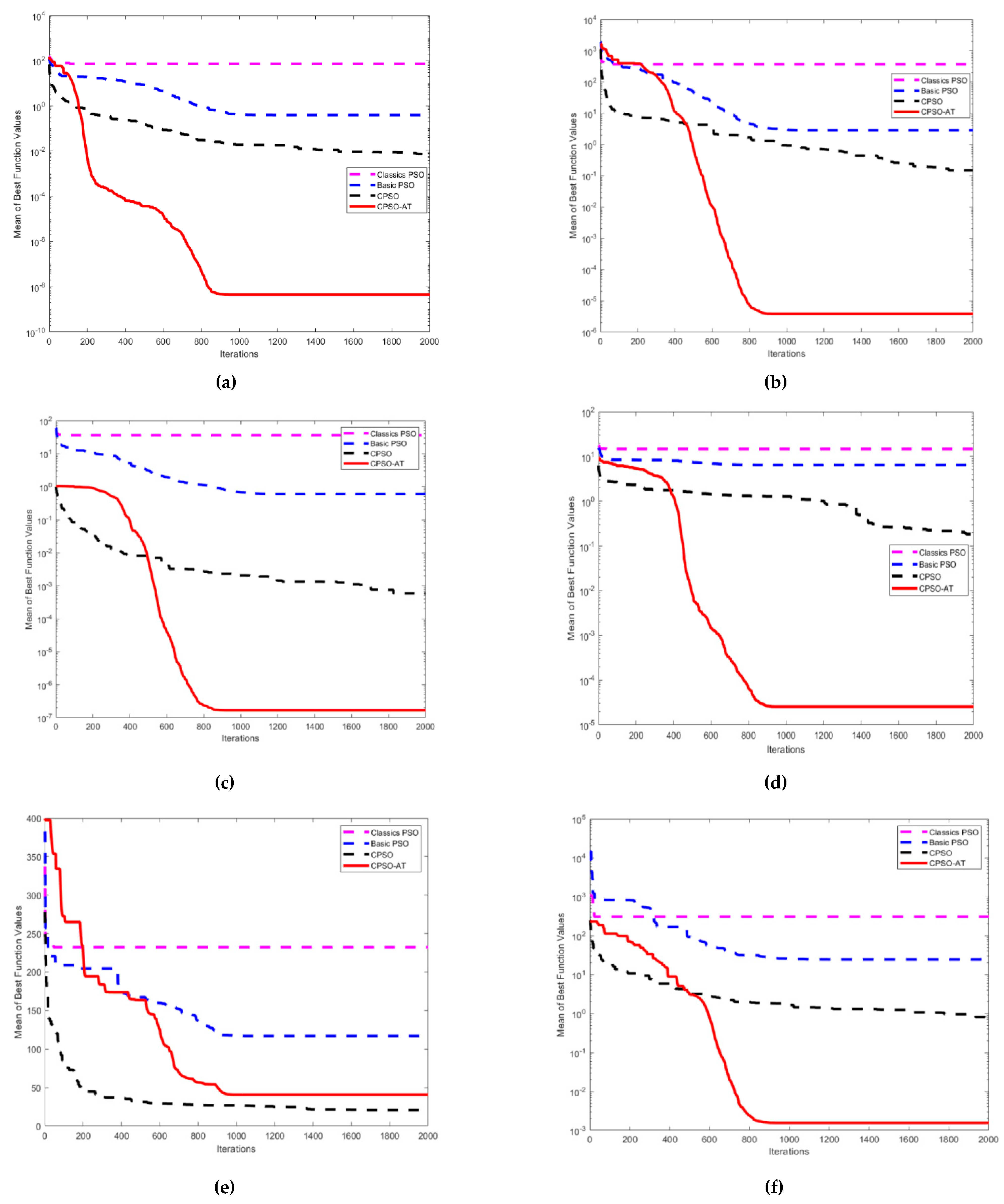
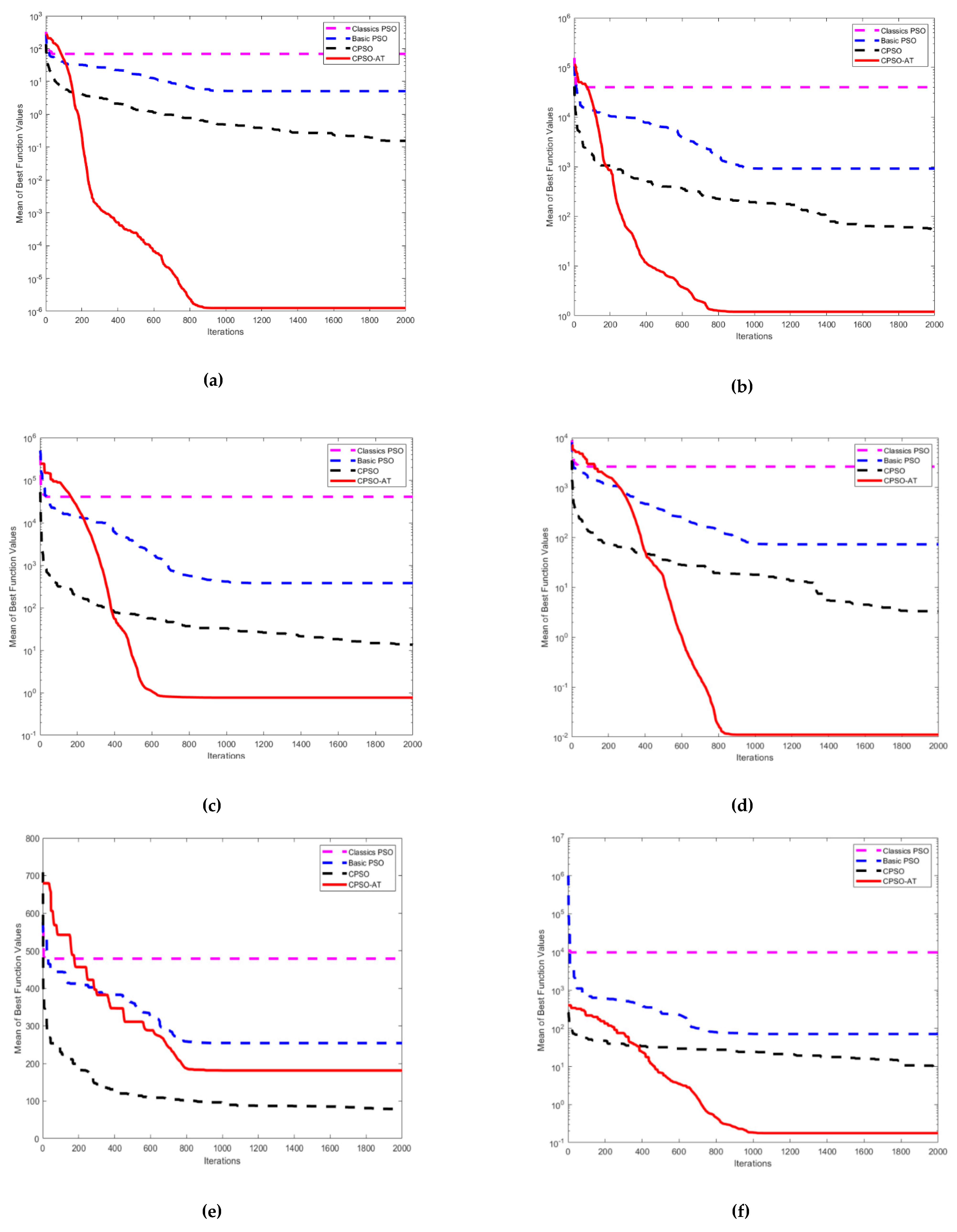
5.1. Comparison of CPSO-AT with Classical PSO, Basic PSO, and CPSO

We conducted many experiments to verify the effectiveness of a chaotic search theory, nonlinear dynamic learning factor, and nonlinear dynamic inertia weight. The algorithms were tested using 10 benchmark functions with 30 and 50 dimensions, and the results are shown in Table 3 and Table 4. Figure 5a–f and Figure 6a–f depict the convergence diagrams of basic PSO, classical PSO, CPSO and CPSO-AT algorithms with 30 and 50 dimensions of test functions. The values indicated in the figures are the mean of the best function values obtained from 30 independent experiments.
Figure 5a,b illustrate that the proposed CPSO-AT stood out when compared with the other three algorithms and its optimization accuracy and convergence speed had obvious advantages for unimodal functions f 1 and f 5 . From Figure 5c,d,f we can see that the proposed CPSO-AT algorithm showed better performance for multimodal functions f 6 , f 7 , f 10 . However, Figure 5e and Figure 6e depict that for f 8 the performance of CPSO-AT was not as good as that of the CPSO algorithm. From Figure 6a,b, it can be seen that the CPSO-AT showed the fastest convergence speed and stronger robustness compared with the other three methods. Figure 6c,d,f demonstrate that the CPSO-AT had a better ability of escaping from the local optimums.
The same conclusion can be drawn from Table 3 and Table 4, which demonstrate the best fitness value (The best), worst fitness value (The worst), mean results (mean) and standard deviations (S.D.) of the CPSO-AT algorithm and three other PSO variants. It can be concluded that the proposed CPSO-AT achieved better optimization results for all unimodal functions f 1 f 5 . For four multimodal functions ( f 6 , f 7 , f 9 , f 10 ) , the CPSO-AT algorithm also outperformed the three other PSO variants. However, for multimodal function f 8 all algorithms had very close optimization accuracy. Moreover, the last columns of Table 3 and Table 4 revealed that the proposed CPSO-AT provided better robustness and stability than basic PSO and its variants.

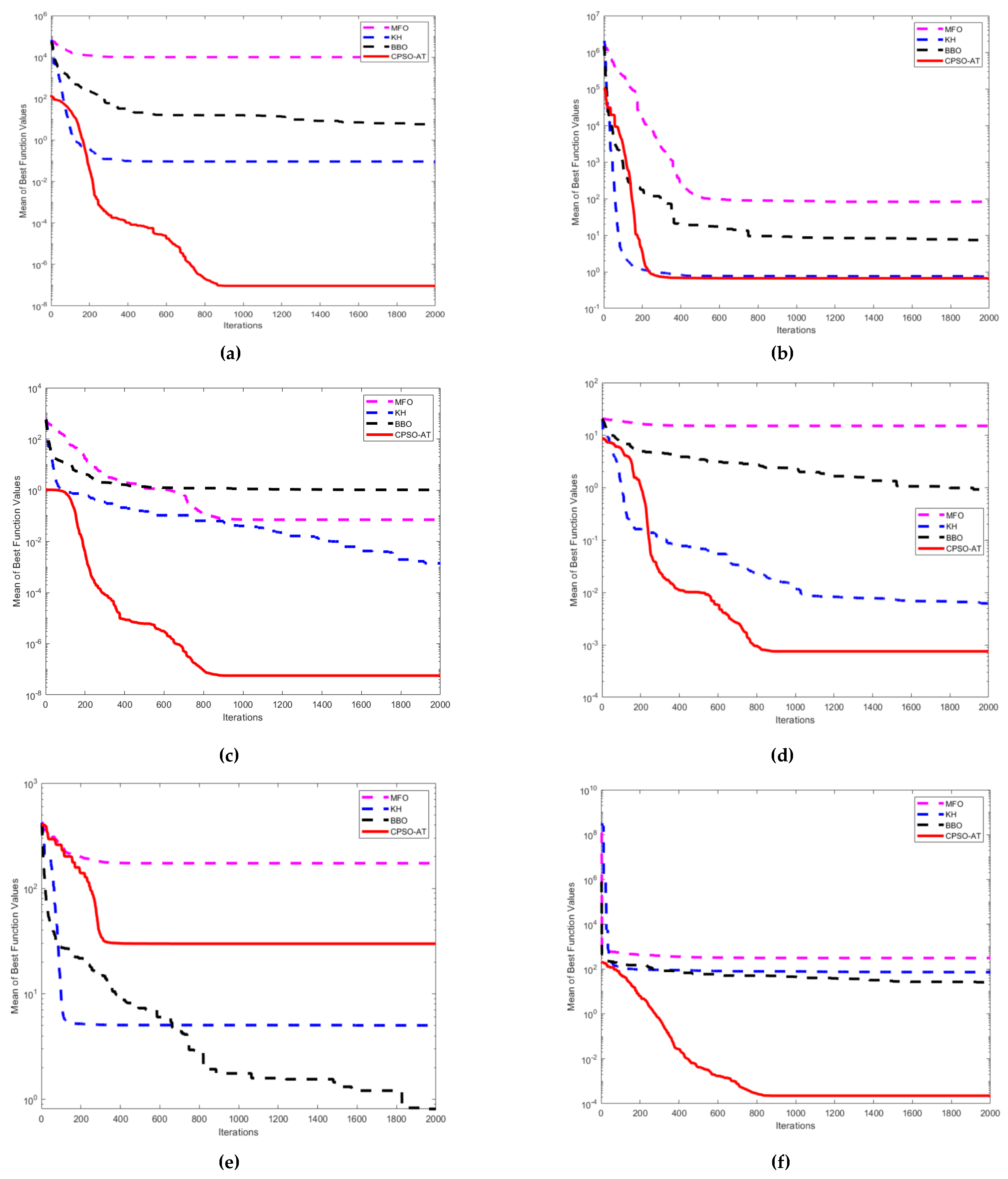
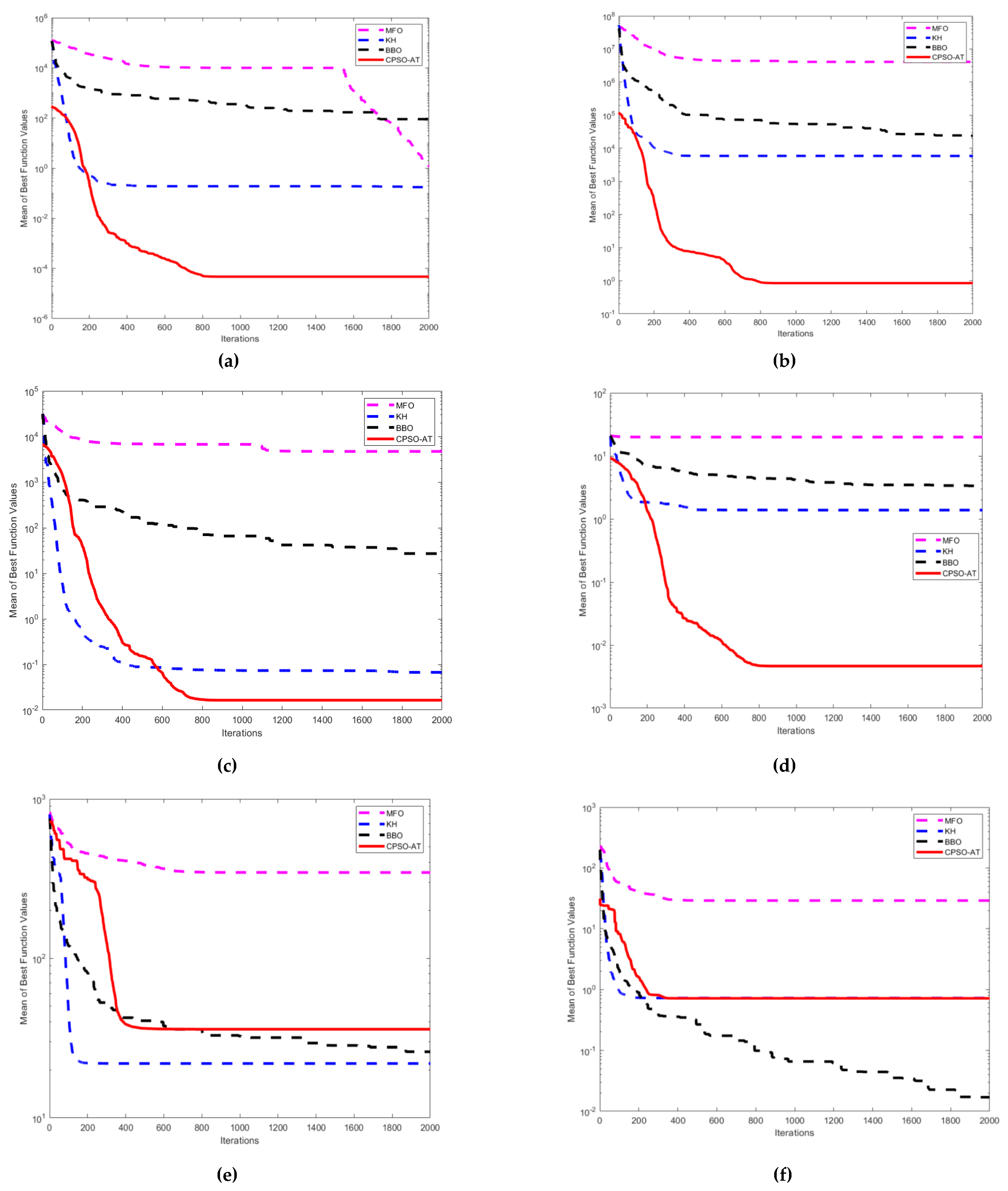
5.2. Comparison of Chaotic Particle Swarm Optimization-Arctangent Acceleration with Moth-Flame Optimization, Krill Herd and Biogeography-Based Optimization

We compared our CPSO-AT algorithm with the optimization algorithms proposed by other researchers. The parameters for moth-flame optimization algorithm (MFO) [12], krill herd (KH) algorithm [11], and biogeography-based optimization (BBO) [8] are shown in Table 6. The 10 classical test functions listed in Table 2 were used for comparison and their dimensions were set to 30 and 50. For a fair comparison, each experiment was repeated 30 times for each test function. The experimental results are shown in Table 6 and Table 7, including the optimal fitness values (the best), worst fitness values (the worst), average results (mean), and standard deviation (S.D.) for the MFO, KH, BBO, and CPSO-AT algorithms. The convergence curves of the above algorithms are illustrated in Figure 7a–f and Figure 8a–f.
The experimental results for solving 10 standard test functions in 30 dimensions are provided in Figure 7a–f and Table 6, which show that the CPSO-AT algorithm had obvious advantages compared with the other three well-known algorithms in all unimodal functions ( f 1 f 5 ) . For multimodal functions, the CPSO-AT algorithm found better solutions for f 6 , f 7 , and f 10 . However, for f 8 and f 9 , the performance was not as good as the BBO and KH algorithms, as shown in Figure 7e and Table 6.
The last two columns of Table 6 show that for the majority of the benchmark functions ( f 1 f 7 , f 10 ) , the proposed CPSO-AT algorithm performed better in both search accuracy and stability. The mean values listed in the sixth column of Table 6 show that for six functions ( f 1 , f 2 , f 5 , f 6 , f 7 , f 10 ) , the CPSO-AT was obviously superior compared with the three other meta-heuristic optimization algorithms. The BBO algorithm produced the best results for two numerical functions ( f 8 , f 9 ) , which made it the second best methodology. However, the optimization results of CPSO-AT were very close to those produced by the BBO algorithm for f 8 and f 9 . KH was ranked as the third most impactful method by providing preferable solutions on four test functions ( f 4 , f 3 , f 8 , f 9 ) , but performed poorly in six functions ( f 1 , f 2 , f 5 , f 6 , f 7 , f 10 ) . MFO did not perform well on almost all test functions, and was determined to be the least effective method.
Table 6 and Table 7 demonstrate that the CPSO-AT algorithm produced the best results among all four methods, followed by BBO, KH, then MFO. Figure 7a depicts the performance of the four algorithms for the f 1 function. During the search, the performance of CPSO-AT was superior. Figure 7b–d,f indicate that BBO, KH, and MFO were inferior to CPSO-AT. Figure 7e shows that BBO and KH performed better than CPSO-AT and MFO, but the optimization effect of CPSO-AT was close to that of the BBO algorithm.
Table 7 presents the optimization results of 10 standard test functions with 50 dimensions, and we concluded that the CPSO-AT algorithm provided a considerable advantage for solving unimodal function problems ( f 1 f 5 ) . However, for multimodal functions f 8 and f 9 , BBO and KH algorithms performed slightly better than CPSO-AT. For the rest of the multimodal functions ( f 6 , f 7 , f 10 ) , the proposed CPSO-AT outperformed the other three heuristic optimization algorithms.
The convergence curves of the mean values of the numerical experiment functions ( f 1 , f 2 , f 5 , f 7 , f 8 , f 10 ) with 50 dimensions are illustrated in Figure 8a–f. Figure 8a, b indicate that the CPSO-AT method provided the best search result compared with the other three methods, whereas the KH method was able to quickly converge to the global optimum. However, Figure 8e shows that the two algorithms (KH and BBO) can find similar solutions, and Figure 8f shows that the BBO algorithm has a powerful ability to globally search to evade the local optimum solution in the 50-dimensional f 10 function. For most situations, the proposed CPSO-AT algorithm provided superior convergence accuracy and a steadier search ability than the other three methods when solving numerical optimization problems.
From Table 6 and Table 7 and Figure 7a–f and Figure 8a–f, we conclude that for numerical function optimization problems, the proposed CPSO-AT algorithm was superior compared with MFO, KH, and BBO. In particular for unimodal functions, the proposed method had obvious advantages. Therefore, when solving single-modal function problems, we recommend using the CPSO-AT algorithm. For multimodal functions, CPSO-AT also performs well in both optimization accuracy and convergence speed. In summary, the CPSO-AT provides a good balance between global exploration and local exploitation capabilities, which indicates that the proposed nonlinear dynamic weights, dynamic learning factors, linear mapping, and chaotic particle position updating method are effective for enhancing the performance of CPSO-AT.

6. Conclusions and Future Work

In this paper, we proposed a novel CPSO-AT algorithm that could improve the overall performance of the traditional PSO method. To obtain a good balance between global and local search capabilities, nonlinear dynamic weights, dynamic learning factors, linear mapping, and chaotic particle position updating methods were combined in the proposed method. Extensive experiments were conducted using ten 30-dimensional and 50-dimensional classical benchmark functions to verify the effectiveness of the proposed method. In the first set of experiments, CPSO-AT was compared with basic PSO and its two kinds of variants, and with three other well-known optimization algorithms in the second group of experiments. The experimental results indicated that applying dynamic weights and dynamic learning factors in the proposed CPSO-AT algorithm were beneficial and better results were obtained for most of the classical benchmark functions. Therefore, the proposed CPSO-AT is a good choice for solving numerical optimization problems.
In the future, the diversity of particles and the convergence speed of the CPSO-AT algorithm needs to be further studied. We plan to apply the CPSO-AT algorithm to solving some real-world problems in future work.

Author Contributions

Z.M. and X.Y. designed the experiments; Z.M., S.H. and D.S. performed the experiments; Y.M. analyzed the data; Z.M. and X.Y. wrote the paper.

Acknowledgments

This work was supported by The National Natural Science Foundation of China (Grant No. 61803227, 61773242, 61603214, 61573213), National Key R & D Program of China (Grant No.2017YFB1302400), Key Program of Scientific and Technological Innovation of Shandong Province (Grant No. 2017CXGC0926), Key Research and Development Program of Shandong Province (Grant No. 2017GGX30133, 2018GGX101039), Independent Innovation Foundation of Shandong University (Grant No. 2082018ZQXM005).

Conflicts of Interest

The authors declare that there were no conflicts of interests regarding the publication of this paper.

References

  1. Wang, G.; Guo, J.M.; Chen, Y.P.; Li, Y.; Xu, Q. A PSO and BFO-based Learning Strategy applied to Faster R-CNN for Object Detection in Autonomous Driving. IEEE Access 2019, 7, 18840–18859. [Google Scholar] [CrossRef]
  2. Siano, P.; Citro, C. Designing fuzzy logic controllers for DC–DC converters using multi-objective particle swarm optimization. Electr. Power Syst. Res. 2014, 112, 74–83. [Google Scholar] [CrossRef]
  3. Yu, Z.H.; Xiao, L.J.; Li, H.Y.; Zhu, X.L.; Huai, R.T. Model Parameter Identification for Lithium Batteries using the Coevolutionary Particle Swarm Optimization Method. IEEE Trans. Ind. Electron. 2017, 64, 569–5700. [Google Scholar] [CrossRef]
  4. Chen, K.; Zhou, F.Y.; Liu, A.L. Chaotic dynamic weight particle swarm optimization for numerical function optimization. Knowl. Based Syst. 2018, 139, 23–40. [Google Scholar] [CrossRef]
  5. Lee, C.S.; Wang, M.H.; Wang, C.S.; Teytaud, O.; Liu, J.L.; Lin, S.W.; Hung, P.H. PSO-based Fuzzy Markup Language for Student Learning Performance Evaluation and Educational Application. IEEE Trans. Fuzzy Syst. 2018, 26, 2618–2633. [Google Scholar] [CrossRef]
  6. Mirjalili, S. SCA: A Sine Cosine Algorithm for solving optimization problems. Knowl. Based Syst. 2016, 96, 120–133. [Google Scholar] [CrossRef]
  7. Dorigo, M.; Maniezzo, V.; Colorni, A. Ant system: Optimization by a colony of cooperating agents. IEEE Trans. Syst. Man Cybern. Part B Cybern. 2002, 26, 29–41. [Google Scholar] [CrossRef]
  8. Simon, D. Biogeography-Based Optimization. Trans. Evol. Comput. 2008, 12, 702–713. [Google Scholar] [CrossRef]
  9. Mirjalili, S.; Mirjalili, S.M.; Lewis, A. Grey Wolf Optimizer. Adv. Eng. Softw. 2014, 69, 46–61. [Google Scholar] [CrossRef] [Green Version]
  10. Das, S.; Mullick, S.S.; Suganthan, P.N. Recent advances in differential evolution—An updated survey. Swarm Evol. Comput. 2016, 27, 1–30. [Google Scholar] [CrossRef]
  11. Gandomi, A.H.; Alavi, A.H. Krill herd: A new bio-inspired optimization algorithm. Commun. Nonlinear Sci. Numer. Simul. 2012, 17, 4831–4845. [Google Scholar] [CrossRef]
  12. Mirjalili, S. Moth-flame optimization algorithm: A novel nature-inspired heuristic paradigm. Knowl. Based Syst. 2015, 89, 228–249. [Google Scholar] [CrossRef]
  13. Mirjalili, S.; Lewis, A. The Whale Optimization Algorithm. Adv. Eng. Softw. 2016, 95, 51–67. [Google Scholar] [CrossRef]
  14. Chen, K.; Zhou, F.Y.; Wang, Y.G.; Yin, L. An ameliorated particle swarm optimizer for solving numerical optimization problems. Appl. Soft Comput. 2018, 73, 482–496. [Google Scholar] [CrossRef]
  15. Bonyadi, M.R.; Michale, Z. Particle Swarm Optimization for Single Objective Continuous Space Problems: A Review. Evol. Comput. 2017, 25, 1–54. [Google Scholar] [CrossRef] [PubMed]
  16. Zhang, X.M.; Feng, T.H.; Niu, Q.S.; Deng, X.J. A Novel Swarm Optimisation Algorithm Based on a Mixed-Distribution Model. Appl. Sci. Basel 2018, 8, 632. [Google Scholar] [CrossRef]
  17. Ozturk, C.; Hancer, E.; Karaboga, D. A novel binary artificial bee colony algorithm based on genetic operators. Inf. Sci. 2015, 297, 154–170. [Google Scholar] [CrossRef]
  18. Tey, K.S.; Mekhilef, S.; Seyedmahmoudian, M.; Horan, B.; Oo, A.M.T.; Stojcevski, A. Improved Differential Evolution-Based MPPT Algorithm Using SEPIC for PV Systems Under Partial Shading Conditions and Load Variation. IEEE Trans. Ind. Inform. 2018, 14, 4322–4333. [Google Scholar] [CrossRef]
  19. Mirjalili, S. The Ant Lion Optimizer. Adv. Eng. Softw. 2015, 83, 80–98. [Google Scholar] [CrossRef]
  20. García-Ródenas, R.; Linares, L.J.; López-Gómez, J.A. A Memetic Chaotic Gravitational Search Algorithm for unconstrained global optimization problems. Appl. Soft Comput. 2019, 79, 14–29. [Google Scholar] [CrossRef]
  21. Tian, M.; Gao, X. Differential evolution with neighborhood-based adaptive evolution mechanism for numerical optimization. Inf. Sci. 2019, 478, 422–448. [Google Scholar] [CrossRef]
  22. Hooker, J.N. Testing heuristics: We have it all wrong. J. Heuristics 1995, 1, 33–42. [Google Scholar] [CrossRef]
  23. Sergeyev, Y.D.; Kvasov, D.E.; Mukhametzhanov, M.S. On the efficiency of nature-inspired metaheuristics in expensive global optimization with limited budget. Sci. Rep. 2018, 8, 453. [Google Scholar] [CrossRef] [PubMed]
  24. Pepelyshev, A.; Zhigljavsky, A.; Žilinskas, A. Performance of global random search algorithms for large dimensions. J. Glob. Optim. 2018, 71, 57–71. [Google Scholar] [CrossRef]
  25. Shi, Y.; Eberhart, R. Modified Particle Swarm Optimizer. In Proceedings of the IEEE International Conference on Evolutionary Computation, Anchorage, AK, USA, 4–9 May 1999; pp. 69–73. [Google Scholar]
  26. Khatami, A.; Mirghasemi, S.; Khosravi, A.; Lim, C.P.; Nahavandi, S. A new PSO-based approach to fire flame detection using K-Medoids clustering. Expert Syst. Appl. 2017, 68, 69–80. [Google Scholar] [CrossRef]
  27. Lin, C.W.; Yang, L.; Fournier-Viger, P.; Hong, T.P.; Voznak, M. A binary PSO approach to mine high-utility itemsets. Soft Comput. 2017, 21, 5103–5121. [Google Scholar] [CrossRef]
  28. Zhou, Y.; Wang, N.; Xiang, W. Clustering Hierarchy Protocol in Wireless Sensor Networks Using an Improved PSO Algorithm. IEEE Access 2017, 5, 2241–2253. [Google Scholar] [CrossRef]
  29. Chouikhi, N.; Ammar, B.; Rokbani, N.; Alimi, A.M. PSO-based analysis of Echo State Network parameters for time series forecasting. Appl. Soft Comput. 2017, 55, 211–225. [Google Scholar] [CrossRef]
  30. Wang, G.G.; Guo, L.; Gandomi, A.H.; Hao, G.S.; Wang, H. Chaotic Krill Herd algorithm. Inf. Sci. 2014, 274, 17–34. [Google Scholar] [CrossRef]
  31. Niu, P.; Chen, K.; Ma, Y.; Li, X.; Liu, A.; Li, G. Model turbine heat rate by fast learning network with tuning based on ameliorated krill herd algorithm. Knowl. Based Syst. 2017, 118, 80–92. [Google Scholar] [CrossRef]
Figure 1. Bifurcation diagram of the logistic map for Equation (4).
Symmetry 11 00876 g001
Figure 2. Bifurcation diagram of the logistic map for Equation (5).
Symmetry 11 00876 g002
Figure 3. Arc tangent function acceleration coefficients (AT).
Symmetry 11 00876 g003
Figure 4. Improved inertia weight image.
Symmetry 11 00876 g004
Figure 5. Comparison of the convergence curves of four algorithms for different test functions (Dim = 30): (a) f 1 ; (b) f 5 ; (c) f 6 ; (d) f 7 ; (e) f 8 ; (f) f 10 .
Symmetry 11 00876 g005
Figure 6. Comparison of the convergence curves of four algorithms for different test functions (Dim = 50): (a) f 1 ; (b) f 2 ; (c) f 4 ; (d) f 5 ; (e) f 8 ; (f) f 10 .
Symmetry 11 00876 g006
Figure 7. Comparison of the convergence curves of four algorithms for different test functions (Dim = 30): (a) f 1 ; (b) f 4 ; (c) f 6 ; (d) f 7 ; (e) f 8 ; (f) f 10 .
Symmetry 11 00876 g007
Figure 8. Comparison of the convergence curves of four algorithms for different test functions (Dim = 50): (a) f 1 ; (b) f 2 ; (c) f 5 ; (d) f 7 ; (e) f 8 ; (f) f 10 .
Symmetry 11 00876 g008
Table 1. Parameter settings for Chaotic Particle Swarm Optimization- Arctangent Acceleration (CPSO-AT) and other Particle Swarm Optimization (PSO) variants.
AlgorithmsPopulation SizeDimensionParameter SettingsIteration
Basic PSO10030,50 c 1 = c 2 = 2.0 , ω = 1 , V max = 0.2 × B o u n d 2000
Classical PSO10030,50 c 1 = c 2 = 2.0 , ω = 0.9 ~ 0.4 , V max = 0.2 × B o u n d 2000
CPSO10030,50 c 1 = c 2 = 2.0 , ω = 0.9 ~ 0.4 , V max = 0.2 × B o u n d 2000
CPSO-AT10030,50 c 1 : 2.5 ~ 0.5 , c 2 = 0.5 ~ 2.5 , ω = 0.9333 ~ 0.2667 , V max = 0.2 × B o u n d 2000
Table 2. Multi-dimensional classical benchmark functions.
NameTest functionDimS f min Group
sphere f 1 ( x ) = i = 1 n x i 2 30
50
[ 100 , 100 ] n 0Unimodal
Schwefel’s 1.2 f 2 ( x ) = i = 1 n ( j = 1 i x j ) 2 30
50
[ 100 , 100 ] n 0Unimodal
Rosenbrock f 3 ( x ) = i = 1 n 1 [ 100 ( x i + 1 x i 2 ) 2 + ( x i 1 ) 2 ] 30
50
[ 30 , 30 ] n 0Unimodal
Dixon & Price f 4 ( x ) = ( x 1 1 ) 2 + i = 2 n i ( 2 x i 2 x i 1 ) 2 30
50
[ 10 , 10 ] n 0Unimodal
Sum Squares f 5 ( x ) = i = 1 n i x i 2 30
50
[ 10 , 10 ] n 0Unimodal
Griewank f 6 ( x ) = i = 1 n x i 2 4000 i = 1 n cos ( x i / i ) 1 30
50
[ 600 , 600 ] n 0Multimodal
Ackley f 7 ( x ) = 20   exp ( 0.2 1 n i = 1 n x i 2 ) exp ( 1 n i = 1 n cos ( 2 π x i ) ) + 20 + e 30
50
[ 32 , 32 ] n 0Multimodal
Rastrigin f 8 ( x ) = i = 1 n ( x i 2 10 cos ( 2 π x i ) + 10 ) 30
50
[ 5.12 , 5.12 ] n 0Multimodal
Levy f 9 ( x ) = sin 2 π ω i i = 1 n 1 ( ω i 1 ) 2 [ 1 + 10 sin 2 ( π ω i + 1 ) ] + ( ω d 1 ) 2 [ 1 + 10 sin 2 ( 2 π ω d ) ]
where   ω i = 1 + x i 1 4 , for   all   i = 1 , , n
30
50
[−10, 10]n0Multimodal
Zakharov f 10 ( x ) = i = 1 n x i 2 + ( i = 1 n 0.5 i x i ) 2 + ( i = 1 n 0.5 i x i ) 4 30
50
[−5, 10]n0Multimodal
Table 3. Experimental results obtained by basic particle swarm optimization (PSO), classical PSO, CPSO, and Chaotic Particle Swarm Optimization-Arctangent Acceleration (CPSO-AT) with 30 dimensions.
FunctionAlgorithmkThe bestThe worstMeanS.D.
f1Basic PSO12.6248 × 10017.7947 × 10014.6323 × 10016.7444 × 1001
Classical PSO2.0757 × 10−026.6373 × 10−011.9719 × 10−017.8747 × 10−01
CPSO5.2121 × 10−032.1287 × 10−021.1753 × 10−028.2205 × 10−04
CPSO-AT6.3925 × 10−103.4988 × 10−084.7194 × 10−093.4958 × 10−08
f2Basic PSO12.2111 × 10039.9471 × 10034.9502 × 10031.0172 × 1004
Classical PSO1.1954 × 10011.6882 × 10025.3816 × 10011.6148 × 1002
CPSO1.1748 × 10005.6324 × 10003.0123 × 10003.0028 × 10−01
CPSO-AT2.4951 × 10−057.2287 × 10−031.2410 × 10−038.8665 × 10−03
f3Basic PSO12.6521 × 10051.6800 × 10069.3596 × 10051.0188 × 1005
Classical PSO3.6194 × 10021.9558 × 10061.1596 × 10061.4155 × 1005
CPSO2.7934 × 10011.4180 × 10025.5210 × 10012.7520 × 1001
CPSO-AT2.0086 × 10012.7560 × 10012.4461 × 10012.4490 × 10−01
f4Basic PSO12.6551 × 10031.1167 × 10052.3649 × 10046.2701 × 1003
Classical PSO7.7642 × 10007.8947 × 10043.3909 × 10046.8874 × 1003
CPSO1.2618 × 10005.2299 × 10002.9283 × 10005.3780 × 10−01
CPSO-AT6.6667 × 10−016.6939 × 10−016.6699 × 10−017.5939 × 10−04
f5Basic PSO11.0021 × 10032.0249 × 10031.5684 × 10036.4703 × 1001
Classical PSO1.7245 × 10012.2872 × 10031.3307 × 10031.8101 × 1002
CPSO1.2397 × 10−014.4059 × 10−012.4581 × 10−013.8646 × 10−02
CPSO-AT4.4910 × 10−064.4064 × 10−041.1348 × 10−042.6671 × 10−05
f6Basic PSO13.2239 × 10015.5316 × 10014.0062 × 10019.2496 × 10−01
Classical PSO1.0188 × 10005.1722 × 10012.7296 × 10012.6616 × 1000
CPSO8.6921 × 10−041.1118 × 10−023.1795 × 10−038.4473 × 10−04
CPSO-AT1.1528 × 10−085.5167 × 10−046.0028 × 10−052.0000 × 10−05
f7Basic PSO18.8528 × 10001.6029 × 10011.1915 × 10015.3159 × 10−01
Classical PSO7.4734 × 10001.2232 × 10011.1736 × 10012.1728 × 10−01
CPSO9.3623 × 10−022.0819 × 10005.1825 × 10−012.2687 × 10−01
CPSO-AT5.2116 × 10−051.8759 × 10−041.0254 × 10−041.6110 × 10−05
f8Basic PSO02.4279 × 10023.2104 × 10022.6438 × 10023.4627 × 1000
Classical PSO6.8569 × 10013.1272 × 10022.9253 × 10024.5919 × 1000
CPSO2.9624 × 10014.2594 × 10013.6522 × 10011.9274 × 1000
CPSO-AT9.2920 × 10011.7194 × 10021.3559 × 10025.0030 × 1000
f9Basic PSO11.0570 × 10015.6268 × 10012.9851 × 10012.6466 × 1000
Classical PSO5.2905 × 10004.9856 × 10012.1421 × 10012.8645 × 1000
CPSO9.4416 × 10−032.7481 × 10008.9063 × 10−011.4012 × 10−01
CPSO-AT3.5811 × 10−018.0576 × 10−015.5508 × 10−014.5298 × 10−01
f10Basic PSO18.5199 × 10012.4830 × 10021.4751 × 10022.0541 × 1001
Classical PSO5.3003 × 10−011.1802 × 10028.4578 × 10016.7666 × 1000
CPSO5.7915 × 10−011.1559 × 10008.3102 × 10−015.2794 × 10−02
CPSO-AT1.3389 × 10−043.6616 × 10−031.2061 × 10−032.1842 × 10−04
Table 4. Experimental results obtained by basic particle swarm optimization (PSO), classical PSO, CPSO, and Chaotic Particle Swarm Optimization- Arctangent Acceleration (CPSO-AT) with 50 dimensions.
FunctionAlgorithmkThe bestThe worstMeanS.D.
f1Basic PSO16.2992 × 10011.4072 × 10029.6568 × 10011.1705 × 1002
Classical PSO1.9810 × 10009.4058 × 10004.7912 × 10001.0715 × 1001
CPSO7.9989 × 10−021.9665 × 10−011.3500 × 10−014.0335 × 10−03
CPSO-AT4.3797 × 10−071.3892 × 10−052.6618 × 10−061.3012 × 10−05
f2Basic PSO11.7735 × 10044.4191 × 10043.3163 × 10044.0007 × 1004
Classical PSO7.0766 × 10022.4271 × 10031.3298 × 10032.2228 × 1003
CPSO3.4384 × 10011.9495 × 10027.9785 × 10015.0406 × 1000
CPSO-AT1.3885 × 10−012.7291 × 10007.4383 × 10−013.4377 × 1000
f3Basic PSO12.9077 × 10061.4292 × 10077.9705 × 10066.3951 × 1005
Classical PSO6.9551 × 10031.6232 × 10076.8072 × 10061.1339 × 1006
CPSO1.0277 × 10023.5589 × 10022.3726 × 10024.4241 × 1001
CPSO-AT4.5713 × 10014.8066 × 10014.6730 × 10011.3927 × 10−01
f4Basic PSO18.5353 × 10046.5400 × 10052.3039 × 10054.4620 × 1004
Classical PSO2.1823 × 10022.5940 × 10051.0611 × 10051.7552 × 1004
CPSO8.5470 × 10003.0465 × 10012.0967 × 10013.9523 × 1000
CPSO-AT6.6783 × 10−012.0588 × 10008.4647 × 10−015.6966 × 10−02
f5Basic PSO12.9846 × 10037.5971 × 10035.4303 × 10033.7474 × 1002
Classical PSO6.5151 × 10017.6068 × 10034.5427 × 10036.5260 × 1002
CPSO3.1804 × 10005.6937 × 10004.2359 × 10001.9161 × 10−01
CPSO-AT4.7685 × 10−036.7831 × 10−022.0803 × 10−025.0860 × 10−03
f6Basic PSO14.3759 × 10011.0136 × 10027.8097 × 10014.6646 × 1000
Classical PSO6.1000 × 10001.0849 × 10028.7209 × 10014.9779 × 1000
CPSO6.9568 × 10−031.4624 × 10−029.6156 × 10−037.3385 × 10−04
CPSO-AT4.4032 × 10−065.4671 × 10−048.9087 × 10−052.3055 × 10−05
f7Basic PSO11.3003 × 10011.5286 × 10011.3916 × 10011.7718 × 10−01
Classical PSO8.0444 × 10001.5888 × 10011.4502 × 10014.5279 × 10−01
CPSO4.6800 × 10−011.9761 × 10001.5023 × 10004.2769 × 10−02
CPSO-AT2.0332 × 10−038.7914 × 10−019.1370 × 10−022.9368 × 10−02
f8Basic PSO05.1852 × 10026.0608 × 10025.7156 × 10021.6262 × 1000
Classical PSO1.1434 × 10025.7794 × 10024.5988 × 10028.5234 × 1000
CPSO7.4647 × 10011.4715 × 10021.1398 × 10027.3222 × 1000
CPSO-AT2.0437 × 10023.2078 × 10022.6771 × 10028.6923 × 1000
f9Basic PSO13.2829 × 10017.5323 × 10015.1270 × 10013.5370 × 1000
Classical PSO3.8076 × 10004.8866 × 10013.6627 × 10012.9257 × 1000
CPSO1.3024 × 10005.1136 × 10002.8866 × 10004.1186 × 10−01
CPSO-AT6.2676 × 10−011.4325 × 10001.0566 × 10008.0876 × 10−01
f10Basic PSO14.3138 × 10039.8686 × 10061.2329 × 10064.0793 × 1005
Classical PSO7.0378 × 10012.9135 × 10056.9641 × 10042.1887 × 1004
CPSO6.6807 × 10001.3292 × 10011.0134 × 10018.8523 × 10−01
CPSO-AT2.2299 × 10−011.3807 × 10006.4995 × 10−013.0979 × 10−02
Table 5. Parameter settings for the four studied algorithms.
AlgorithmPopulationMaximum IterationsDimOther
MFO50200030,50 t is random number in the range [−2,1]
KH50200030,50 N m a x = 0.01 , V f = 0.02 , D m a x = 0.005
BBO50200030,50 Mu = 0.005 , μ = 0.8 c
CPSO-AT50200030,50 ω = φ × cos ( ( M j M m a x ) × π ) + τ
c 1 = × arctan ( ( M J M m a x ) × σ ) + δ 1
c 2 = × arctan ( ( M j M m a x ) × σ ) + δ 2
Table 6. Experimental results produced by the Moth-Flame Optimization Algorithm (MFO), Krill Herd Algorithm (KH) and Biogeography-Based Optimization Algorithm (BBO) and Chaotic Particle Swarm Optimization-Arctangent Acceleration (CPSO-AT) with 30 dimensions.
FunctionAlgorithmkThe BestThe WorstMeanS.D.
f1MFO16.3466 × 10−151.0000 × 10042.0000 × 10031.2649 × 1004
KH9.6793 × 10−034.4021 × 10−022.0048 × 10−021.3669 × 10−02
BBO2.7007 × 10009.8717 × 10004.2946 × 10006.1697 × 1000
CPSO-AT3.1695 × 10−072.8893 × 10−068.6404 × 10−071.1386 × 10−07
f2MFO13.7805 × 10−131.1700 × 10064.7500 × 10051.4342 × 1006
KH7.4251 × 10007.7804 × 10023.1717 × 10023.4905 × 1002
BBO2.4456 × 10021.0627 × 10036.9743 × 10027.0483 × 1002
CPSO-AT1.2328 × 10−031.4670 × 10−013.7457 × 10−029.9016 × 10−03
f3MFO11.6385 × 10031.6385 × 10031.6385 × 10031.7316 × 10−12
KH2.9288 × 10011.2114 × 10025.5490 × 10014.0249 × 1001
BBO1.2701 × 10026.5835 × 10023.2701 × 10025.1255 × 1002
CPSO-AT2.3345 × 10012.9404 × 10012.4992 × 10019.1291 × 10−02
f4MFO16.6667 × 10−012.7370 × 10053.4679 × 10042.6107 × 1005
KH6.7509 × 10−011.2386 × 10008.4426 × 10−012.3154 × 10−01
BBO4.4060 × 10009.1277 × 10006.9919 × 10004.7954 × 1000
CPSO-AT6.6664 × 10−016.6762 × 10−016.6692 × 10−012.1520 × 10−04
f5MFO11.1144 × 10−142.9000 × 10036.9000 × 10022.6738 × 1003
KH8.0391 × 10−032.6790 × 10−017.1299 × 10−021.1182 × 10−01
BBO3.3696 × 10−016.0732 × 10−014.6529 × 10−012.5268 × 10−01
CPSO-AT1.9718 × 10−051.8382 × 10−048.3644 × 10−052.0107 × 10−05
f6MFO19.3259 × 10−159.0535 × 10012.7080 × 10011.3078 × 1002
KH2.0406 × 10−032.3335 × 10−021.0695 × 10−028.9323 × 10−03
BBO1.0110 × 10001.0698 × 10001.0388 × 10004.8482 × 10−02
CPSO-AT8.4554 × 10−081.5809 × 10−063.6554 × 10−075.6011 × 10−08
f7MFO17.0957 × 10−091.9963 × 10019.4662 × 10002.9308 × 1001
KH2.0726 × 10−031.6499 × 10007.0606 × 10−017.0425 × 10−01
BBO7.0705 × 10−011.3181 × 10009.6088 × 10−014.6179 × 10−01
CPSO-AT2.9201 × 10−041.2453 × 10−035.9240 × 10−042.0650 × 10−04
f8MFO07.6612 × 10011.9331 × 10021.3427 × 10029.8256 × 1001
KH5.9930 × 10001.7947 × 10011.2761 × 10014.3635 × 1000
BBO1.0071 × 10002.2005 × 10001.7721 × 10001.2180 × 1000
CPSO-AT9.9508 × 10003.7812 × 10012.0800 × 10012.5423 × 1000
f9MFO02.5135 × 10013.7618 × 10013.0205 × 10019.4966 × 1000
KH2.2932 × 10−048.1506 × 10−012.0720 × 10−012.2620 × 10−01
BBO8.6060 × 10−032.8077 × 10−022.1078 × 10−022.0072 × 10−02
CPSO-AT2.6859 × 10−018.0576 × 10−015.3717 × 10−016.5790 × 10−01
f10MFO11.1036 × 10−024.7619 × 10022.6749 × 10024.3400 × 1002
KH6.6967 × 10011.3059 × 10029.7460 × 10012.5847 × 1001
BBO2.3055 × 10014.4664 × 10013.3702 × 10012.0264 × 1001
CPSO-AT9.4240 × 10−052.1734 × 10−041.7080 × 10−044.8481 × 10−06
Table 7. Experimental results of the Moth-Flame Optimization Algorithm (MFO), Krill Herd Algorithm (KH) and Biogeography-Based Optimization Algorithm (BBO), and Chaotic Particle Swarm Optimization-Arctangent Acceleration (CPSO-AT) with 50 dimensions.
FunctionAlgorithmkThe BestThe WorstMeanS.D.
f1MFO19.0418 × 10−052.0000 × 10041.0000 × 10042.0000 × 1004
KH9.1848 × 10−023.8079 × 10−012.2432 × 10−011.0846 × 10−01
BBO6.8687 × 10011.4266 × 10029.9904 × 10016.6770 × 1001
CPSO-AT1.7020 × 10−055.5462 × 10−054.3225 × 10−058.3417 × 10−07
f2MFO11.0000 × 10045.0200 × 10061.8190 × 10064.6469 × 1006
KH1.0638 × 10038.3849 × 10033.1824 × 10033.0333 × 1003
BBO1.6172 × 10045.0529 × 10042.7620 × 10042.7312 × 1004
CPSO-AT1.0216 × 10004.4131 × 10002.3541 × 10002.6353 × 10−01
f3MFO12.7684 × 10032.7686 × 10032.7684 × 10031.3105 × 10−01
KH6.0262 × 10011.8692 × 10021.3323 × 10024.8077 × 1001
BBO1.4617 × 10034.8529 × 10032.5030 × 10032.7857 × 1003
CPSO-AT4.5596 × 10011.0267 × 10025.2237 × 10012.1782 × 1000
f4MFO16.2704 × 10004.6889 × 10051.8365 × 10054.7211 × 1005
KH2.3253 × 10005.6925 × 10003.2332 × 10001.4030 × 1000
BBO4.7422 × 10011.0958 × 10027.4611 × 10014.8684 × 1001
CPSO-AT6.6895 × 10−018.9973 × 10−017.4677 × 10−014.9214 × 10−02
f5MFO11.8984 × 10−059.7000 × 10032.2300 × 10038.7864 × 1003
KH5.1658 × 10−024.7215 × 10−012.2164 × 10−011.6813 × 10−01
BBO2.1286 × 10013.1796 × 10012.6284 × 10019.5861 × 1000
CPSO-AT3.1182 × 10−033.4762 × 10−021.5271 × 10−022.2791 × 10−03
f6MFO12.6725 × 10−059.0793 × 10012.7162 × 10011.3102 × 1002
KH8.7800 × 10−035.1455 × 10−022.3202 × 10−021.7232 × 10−02
BBO1.8720 × 10002.5471 × 10002.2098 × 10005.5828 × 10−01
CPSO-AT2.7021 × 10−067.4758 × 10−037.5390 × 10−042.4893 × 10−04
f7MFO13.1461 × 10001.9963 × 10011.7381 × 10011.5640 × 1001
KH1.1614 × 10002.9876 × 10001.8086 × 10006.9580 × 10−01
BBO2.9456 × 10003.5964 × 10003.2432 × 10005.4301 × 10−01
CPSO-AT2.4651 × 10−035.1956 × 10−033.7252 × 10−034.6693 × 10−04
f8MFO02.0610 × 10024.0942 × 10022.7372 × 10021.7473 × 1002
KH1.6014 × 10013.4316 × 10012.4666 × 10016.5266 × 1000
BBO1.6638 × 10012.8529 × 10012.4282 × 10019.1892 × 1000
CPSO-AT2.4890 × 10014.4884 × 10013.4785 × 10019.8221 × 10−01
f9MFO01.2546 × 10018.8610 × 10013.2530 × 10016.3687 × 1001
KH4.4904 × 10−012.7557 × 10001.0771 × 10008.7791 × 10−01
BBO3.0271 × 10−016.0636 × 10−014.4337 × 10−012.8994 × 10−01
CPSO-AT5.3723 × 10−011.3432 × 10009.6706 × 10−017.5773 × 10−01
f10MFO16.2671 × 10029.7623 × 10027.9242 × 10024.5047 × 1002
KH3.0410 × 10023.9719 × 10023.4173 × 10023.5971 × 1001
BBO7.6162 × 10011.3712 × 10021.0980 × 10024.7729 × 1001
CPSO-AT9.2969 × 10−036.3677 × 10−022.5705 × 10−021.2072 × 10−02

