Article

Optimal Incentive Contract for Sales Team with Loss Aversion Preference

1
School of Business, Hunan University of Science and Technology, Xiangtan 411201, China
2
School of Economic Mathematics, Southwestern University of Finance and Economics, Chengdu 611130, China
3
Hunan Engineering Research Center for Intelligent Decision Making and Big Data on Industrial Development, Xiangtan 411201, China
4
School of Geosciences and Info-Physics, Central South University, Changsha 410083, China
*
Author to whom correspondence should be addressed.
Symmetry 2019, 11(7), 864; https://doi.org/10.3390/sym11070864
Submission received: 14 May 2019 / Revised: 19 June 2019 / Accepted: 20 June 2019 / Published: 3 July 2019

Abstract

:
When manufacturing enterprises employ sales team (or multiple salesmen) to sell products, there is asymmetric information such as the ability and efforts salesmen. Enterprises can use contracts to incentivize salesmen to work hard to maximize their profits. Assuming that market demand is sensitive to effort, and the salesman can exploit the market by increasing effort, a multi-agent model is established for the case of symmetrical information and asymmetrical information, in which the sales team has a loss aversion preference. In this multi-agent model, the agents’ utility function is non-concave and cannot be solved by traditional methods. We use a backward stochastic differential equation (BSDE) to represent agents’ contract through the martingale representation theorem and use the stochastic optimal control and matrix method to obtain the explicit solution of the optimal contract. Based on the conclusions of the research, an empirical analysis is made on the sales team of an enterprise.

1. Introduction

With the globalization of economy and the highly marketization of commodities, the working attitude of sales team, as the external performance of enterprises, will directly affect whether the users approve the enterprises and purchase their products, which in turn affects the economic benefits of enterprises, and even the survival of enterprises. Therefore, it is very critical and important for enterprises to design a scientific and reasonable incentive mechanisms for salesmen, to fully mobilize the enthusiasm of salesmen.
Many empirical studies have shown that the efforts of salesmen have a significant impact on the development of enterprises, for example, Lal and Srinivasan [1], Chan et al. [2], Chung and Narayandas [3]. In the actual market environment, sometimes there is a conflict between encouraging sales staff to work hard and guiding them to disclose the real market information. In order to motivate salesmen to work hard, enterprises must timely reward them according to their sales performance. However, this is not always proportional to the efforts of salesmen. For example, in a tough economy, the hard work of high-level salesmen may only produce relatively low sales performance. Therefore, enterprise managers cannot directly establish the incentive contract on the behavior of the salesmen but rely on the noise performance results to motivate their work.
The research on optimal incentive contracts for salesmen in market and economic literature mainly focuses on the following aspects: the moral hazard problem caused by the unobservability of a salesman’s effort, the dynamic optimal incentive problem of salesmen, and the corresponding contract problem of salesmen for relevant enterprises through empirical investigation. Research by such as scholars Basu et al. [4], Coughlan and Narasimhan [5], Chen [6], Rubel and Prasad [7], and Kräkel and Schöttner [8]. Some scholars have also studied the incentives for different sales ability of salesmen. For example, scholars Albers [9] and Rouziès et al. [10] studied a commonly used incentive contract, in which enterprises set sales targets for salesmen and provide corresponding reward for salesmen who achieved the target. This incentive contract is particularly suitable for salesmen with different sales abilities. Based on the goal-setting theory, Bommaraju and Hohenberg [11] proposed a new self-selection incentive scheme. To verify the results, the author conducted experiments in two of the top 500 enterprises.
With the development of the economy and the expansion of enterprise scale, enterprises and scholars also pay more and more attention to research on the incentive of sales teams or multi-salesman. On the one hand, literature on sales team motivation focuses on multi-salesman working together to achieve total sales results. For example, Holmstrom [12], McAfee and McMillan [13], and Itoh [14]. The research shows that when the efforts of the salesmen are complementary in the sales’ process, team cooperative sales will occur. Without any restraint mechanism, cooperative sales tend to generate free-rider behavior, which is lower than the overall optimal effort level. In this case, team committees help to adjust rewards for team members, conversely, when salesmen are risk-neutral, the lack of complementarities in sales means that team incentive commissions are not optimal. Tian et al. [15] studied the problem of principal-agents with multi-salesman sales, and there is competition between salesmen in the sales system, and given the conclusion that enterprises suffer losses due to lack of information in the case of asymmetric information, they can use the competition between salesmen to reduce the losses of enterprises. Caldieraro and Coughlan [16] studied and investigated the diversification of sales teams and the relevant compensation and incentive strategies of companies deploying sales team to different regions.
On the other hand, with the rise of behavioral economics, many scholars have included behavioral economics into the principal-agent model. For example, Köszegi and Rabin [17,18,19] who first included reference dependence and loss aversion in the traditional principal-agent model, expanded the compatible definition of incentive, and proposed the concept of choosing adaptive individual equilibrium. By assuming that salesmen have a loss aversion preference, Herweg et al. [20] expanded the principal-agent model under moral hazard. Dittmann et al. [21] analyzed the optimal compensation contract when the sales manager has loss aversion. Daido and Murooka [22] studied a multi-agent model, in which salesmen have expected reference preference. The study found that low-performing salesmen could get high rewards by “free riding” when other salesmen achieved high performance. Goukasian and Wan [23] studied the optimal incentive contract under relative income. They assumed that salesman exhibited behavioral biases: Showing embarrassment or admiration for colleagues’ rewards, and the study found that the best efforts of the salesman are negatively affected by the behavioral biases judged by other salesmen. It also showed that jealous behavior is harmful to the sales team. Elie and Possamai [24,25] studied the contract problem of competing multi-agents. Considering the relative performance of salesmen in the competition, the explicit solution of the optimal contract is obtained by using the Nash equilibrium and backward stochastic differential equation. Research shows that every salesman will get reservation utility, while those with higher competitiveness will be assigned to less stable sales items and even get help from other salesmen.
Our model has some characteristics in common with the above principal-agent model, because we consider a stochastic process in which the efforts of salesmen are part of the drift item, and both the enterprise manager and the salesmen have a continuous risk-aversion utility function. However, differing from the above research, we assume that the utility function of all salesmen can be divided into two parts, one is the traditional material utility (consumption, income, etc.), and the other is the “gain-loss” utility in psychology. Considering the “gain-loss” utility function, the salesman’s utility function is non-concave, so the first-order method cannot be solved. In order to obtain the explicit solution of the optimal incentive contract of the sales team, we will use the stochastic optimal control and backward stochastic differential equation (BSDE) and matrix method.
The structure of our paper is as follows: Section 2 presents the continuous time multi-agent model. Section 3 discusses the optimal contracts in the case with information symmetry and taking it as a benchmark. We discuss the design of the optimal contract under the hidden-action case in Section 4, and we analyze the optimal contract for some special cases through the numerical simulation. Finally, we conclude this paper in Section 5. In addition, all proof details in the main text are given in the Appendix.

2. The Model

We consider a model where an enterprise manager employs N salesmen to form a sales team and participate in N different sales projects.
For each salesman, if they accept the contract provided by the manager, they will pay for the effort to affect the output of the project. In this section, we give the definition of the dynamics of the sales revenue processes and also characterize the objective function of each salesman, as well as the manager. In order to identify our model more accurately, we fixed some notations firstly.

2.1. Sales Revenue Process

Considering a finite time horizon [ 0 , T ] , all salesmen carry out their tasks under uncertainty, here we give a probability space ( Ω , , ) , and on which defined an N -dimensional Brownian motion B t = ( B t 1 , , B t N ) , { t } is a suitably augmented filtration generated by the Brownian motion B t . At the initial moment t = 0 , the manager hires N salesmen whom participate in N different sales projects simultaneously, sales revenue of the salesmen’s efforts over time are described by the N -vector cumulative proceeds { Y t } (so-called sales revenue process), its evolution over time [ 0 , T ] is as follows:
d Y t = Σ t d B t
where Y t = ( Y t 1 , , Y t N ) is an N -dimensional outcome vector at time t , and Σ t N ( R ) ( here ,   N ( R ) represents a set of N -order real matrix) is an N × N volatility matrix, which is assumed to be bounded and invertible.
We assume that each salesman has been assigned to all sales projects, and then each salesman’s effort can affect the returns of all sales projects. The efforts of all salesmen can be given by a matrix A N × N , for i , j = 1 , , N . The u i , j is an element of A N × N , which represents the effort provided by salesman i in project j . We consider two information structures: Symmetric information and hidden action, where symmetric information means that all the information in the model is symmetric, and under hidden action the manager can observe the sales revenue process Y t but cannot observe the efforts of all salesmen or the uncertainty which impact the sales revenue under hidden action. The manager cannot distinguish the level of influence of effort and uncertainty on the sales revenue process.
According to the above, the salesmen joined, change the measure from to u by exerting effort, with
d u d = exp ( 0 T ( Σ 1 b ( t , A , u t ) ) d B t 1 2 0 T | Σ 1 b ( t , A , u t ) | 2 d t )
where b : [ 0 , T ] × R N × R N R is a bounded and continuous function. Under hidden action, u cannot be verified.
By Girsanov’s Proposition under u
B t u = B t 0 t Σ 1 b ( s , A , u s ) d s , 0 t T
is a vector of Brownian motion, and we can rewrite the equation as:
d Y t = b ( t , A , u t ) d t + Σ d B t u .
To describe the model more accurately, we denote that
u t = ( u t 1 u t N ) = ( u t 1 , 1 u t 1 , N u t N , 1 u t N , N ) A N × N
and = ( a 11 a 1 N a N 1 a N N )
Σ = ( σ 11 σ 1 N σ N 1 σ N N ) b ( t , A , u t ) = ( b 1 ( t , A , u t ) b 2 ( t , A , u t ) ) = ( a 11 u t 1 , 1 + + a 1 N u t 1 , N a N 1 u t N , 1 + + a N N u t N , N ) .
Then, the sales revenue process can be rewritten as
{ d Y t 1 = ( a 11 u t 1 , 1 + + a 1 N u t 1 , N ) d t + σ 11 d B t u , 1 + + σ 1 N d B t u , N d Y t N = ( a N 1 u t N , 1 + + a N N u t N , N ) d t + σ N 1 d B t u , 1 + + σ N N d B t u , N
where the parameters a i j ( i , j = 1 , , N ) represent the marketing efficiency of salesman i on sales project j . The total sales revenue generated by N salesmen is Y t 1 + + Y t N at time t.

2.2. The Objective Function of Salesman

Given a contract C = ( C 1 , , C N ) , a choice is made whether to accept the contract for each salesman. If accepted, an effort process u t is employed to maximize his expected utility. The salesman’s utility is composed of contracts and the cost of effort. Therefore, we assume that the utilities of the salesmen are exponential, the utility function of salesman i ( i = 1 , , N ) is
U i ( C , u ) = U i ( C i , C i , u i , u i ) = E u [ U i ( C i G T i ) + V i ( C i , C i ) ]
where u i = ( u 1 , u i 1 , u i + 1 , , u N ) are the salary (or contract) and the effort of salesman i ’s co-worker, respectively, and G T i is the cumulative dis-utility of the effort for salesman i , which is defined as:
G T i = 0 T g i ( u i ) d t = 0 T [ j = 1 N g j , i ( u t j , i ) ] d t = 0 T ( j = 1 N k i 2 ( u t j , i ) 2 ) d t
U i corresponds to the classical notion of the outcome-based utility of salesman i , is defined as:
U i ( x ) exp ( r i x ) , x R
r i > 0 is the risk aversion of salesman i . Here the salesman’s material utility function and gain-loss function are assumed as separable and additive [17]. V is a universal gain-loss function which satisfies the assumption introduction by [26]. We say V represents the salesman i ’s gain-loss utility.
The definition of the gain-loss function for salesman defined i as follows:
V i ( C i , C i ) = { e r i ( C i C i ) + 1 if   C i C i , λ ( e r i ( C i C i ) + 1 ) if   C i C i .
where λ 1 is the loss avoidance coefficient. Here C i = C 1 + + C i 1 + C i + 1 + + C N N 1 represents the average value of contracts of other salesmen and also a reference point of salesman i . If the payoff of salesman i exceeds the reference point, which will bring him positive utility, whereas the lower payoff brings a negative utility.

2.3. The Objective Function of Manager

For the manager, he offers a contract C = ( C 1 , , C N ) for each salesman simultaneously at the initial time. He can offer any type of contract, but the contract he provided needs to meet the following three conditions:
First, the manager wants each salesman to accept the contract, then the manager will restrict his contract, so that the contract received by each salesman i ( i = 1 , , N ) is at least the salesman’s reservation utility U - i (Participation Constraint), for i :
U i ( C i , C i , u i , u i ) U - i
Second, under hidden action, the manager sets a recommended effort u ¯ but cannot directly verify if the salesmen were to deviate, thus the manager structures the contract C to provide incentives for salesmen to meet their effort target (Incentive Constraint). For i :
u ¯ i arg max u i   U i ( C i , C i , u i , u i )
Third, we assume that the manager has exponential utility as follows
U P ( Y T , C ) = E u [ e r P · j = 1 N ( Y T j C j ) ]
where r P > 0 is the risk aversion of the manager.
The problem that the manager needs to solve is to choose a suitable contract C ¯ to maximize his expected utility, which is:
C ¯ arg max C   U P ( Y T , C )
We first study a case where there is no hidden action and the manager can verify all the information. We call this kind of case as the first-best, which can be used as a benchmark.

3. Risk Sharing under Symmetric Information

3.1. First-Best Contract

In this section, we discuss the optimal contract, finding the first-best solutions of a case with multiple salesmen under symmetric information, and use it as the benchmark. Given the salesman i ’s reservation utility U - i ( i = 1 , 2 ), the problem of the manager is that
max Y T , C , { u t } t 0 T E u [ e r P ( Y T 1 + Y T 2 C 1 C 2 ) ]
such that
E u [ U i ( C i G T i ) + V i ( C i , C i ) ] U - i ,    i = 1 , 2
where U - i ( L i ) = e r i L i . Without loss of generality, we assume that C 1 C 2 . The risk sharing problem is
Problem 1:
max Y T , C , u t j ( Y T , C , u t ) = max Y T , C , u t E u [ U P ( Y T , C ) + i = 1 2 ρ i U i ( C i G T i ) + ρ 1 ( e r 1 ( C 1 C 2 ) + 1 ) + ρ 2 [ λ ( e r 2 ( C 1 C 2 ) + 1 ) ] + δ ( C 1 C 2 ) ]
where ρ i , δ 0 are the Lagrange multiplier associated participation constraints with condition C 1 C 2 . The following Proposition can be provided:
Proposition 1.
Under symmetric information (First-best case), an optimal contract C F B in Problem 1 with reservation utility U i ( i = 1 , 2 ) is given by
C F B i = 1 r i l n ( ρ i r i r P ) + G T i + r P r i ( 1 + r ¯ ) [ Y T 1 + Y T 2 + ( G T 1 + G T 2 ) + i = 1 2 1 r i l n ( ρ i r i r P ) ]
where the multiplier 1 r i l n ( ρ i r i r P ) satisfies the system of Equation (A5). The first-best optimal efforts u F B are given by:
u F B = ( u F B 1 u F B 2 ) = ( a 11 k 1 a 12 k 2 a 21 k 1 a 22 k 2 )
Proof in Appendix B.1.
Given from Proposition 1, the first-best optimal effort of each salesman depends on his productivity under symmetric information, and it has nothing to do with whether the salesman has gain-loss utility. Under symmetric information, the manager can observe the salesmen’s efforts. Therefore, each salesman will perform the recommended efforts of the manager. Obviously, under symmetric information, the manager does not consider the salesmen’s fair preference when considering the recommended efforts.

3.2. A Special Case

In this subsection, we discuss an explicitly computed optimal contract. The salesmen are set to be exactly the same, means that r 1 = r 2 , L 1 = L 2 , k 1 = k 2 , and λ = 1 .
Proposition 2.
(i): For the absolutely same salesmen, the first-best contract is:
{ C F B 1 = G T 1 1 r 1 l n ( e r 1 L 1 + 1 e r 1 ( G T 1 G T 2 ) ) C F B 1 = G T 2 1 r 2 l n ( e r 2 L 2 1 + e r 2 ( G T 1 G T 2 ) )
where G T 1 = T ( a 11 2 + a 21 2 ) 2 k 1 and G T 2 = T ( a 12 2 + a 22 2 ) 2 k 2 , and the first-best optimal efforts satisfy Equation (5).
(ii) Under symmetric information, if both salesmen do not consider each other’s salaries, or salesmen have no gain-loss utility (rational salesman). If we let U 0 P ( Y T , C ¯ ) represent the expected utility of the manager with the rational salesman, then we have:
U P ( Y T , C F B ) U 0 P ( Y T , C ¯ )
Proof in Appendix B.2.
We can see from Proposition 2, if the salesman i ’s productivity is greater than salesman j , ( a i 1 + a i 2 a j 1 + a j 2 ), then the salesman i ’s efforts cost is more than salesman j ( G T i > G T j ). The manager should pay more salary to salesman i , which can lead the existence of gain-loss utility of the salesman. Here no matter for salesman i or salesman j , the expected utility of the manager will always be less than that of the salesmen without gain-loss utility.
On the other hand, for salesman i , although he received the higher salary than salesman j , however, compared with no gain-loss utility, C F B 1 < C ¯ 1 . In other words, under the influence of gain-loss utility, the salary of salesman i is less than he should be earned. Salesman j is paid more than he deserves due to the gain-loss utility. Salesman i ’s situation is similar to “Winner’s Curse” under symmetric information. If there are differences between salesmen, then we can not determine whether U 0 P ( Y T , C ) is greater than U P ( Y T , C ) , which requires our further study.

4. Contracting Under Hidden Action

In this section, we consider a dynamic model with moral hazard setting, where the manager can observe the sales revenue process Y t , but cannot observe the salesmen’s effort u t i . The salesmen have a separable utility (material utility and gain-loss utility) and a quadratic cost. Different with the one salesman model, according to the first-best contract form, the comparison of salary between salesmen will affect the salesman’s choice and further influence the optimal contract. Since the salesmen at the same time activities, we can find an equilibrium recommend effort between the salesmen and give an optimal contract (so-called second-best contract) to maximize the expected utility of the manager and the salesmen. We give the definition of Nash equilibrium effort for salesmen, refer to [23,25].

4.1. Nash Equilibrium Effort for the Salesmen

Given a contract C = ( C 1 , , C N ) , we define ( u ¯ 1 , , u ¯ N ) as a Nash equilibrium effort for salesmen, for i = 1 , 2 , we have:
U i ( C i , C i , u ¯ i , u ¯ i ) = sup u i A i U i ( C i , C i , u i , u ¯ i )
Shown above, if the contract can motivate salesmen to choose Nash equilibrium effort, then the contract can satisfy the incentive constraint for salesmen. For getting the Nash equilibrium effort for salesmen, we re-analyze the salesmen’s problem. Given a contract C = ( C i , C i ) and the other salesman’s action u i A i (here, A i represents the set of the i th column of the matrix in set A , and A i represents the set of the matrix remove the i th column in set A ), the salesman i aims solving:
U 0 i ( C i , C i , u i , u i ) = sup u i A i   E u i , u i [ e r i ( C i 0 T g i ( u i ) d t ) + V i ( C i , C i ) ]
Similar to [25], the definition of a value function for salesman i is:
U t i ( C i , C i , u i , u i ) = sup u i A i   E u i , u i [ e r i ( C i t T g i ( u i ) d t ) + V i ( C i ) | t ]
Then, e r i 0 t g i d s [ U t i ( C i , C i , u i , u i ) V i ( C i ) ] + V i ( C i ) is a ( F , u i , u i ) -martingale by using martingale representation Proposition, there exist an F - predictable process that Z ˜ i = ( Z ˜ 1 , i , , Z ˜ N , i ) , and applying Ito’s formula:
U t i ( C i , C i , u i , u i ) = ( e r i C i + V i ( C i ) + t T r i g i ( u s i ) [ U s i ( C i , C i , u i , u i ) V i ( C i ) ] d s t T e r i 0 s g i ( u τ i ) d τ Z ˜ s i Σ s d B s u i , u i ,    0 t T
According the definition of B u i , u i , we have, for 0 t T
U t i ( C i , C i , u i , u i ) V i ( C i ) = e r i C i + t T r i [ U s i ( C i , C i , u i , u i ) V i ( C i ) ] Z s i Σ s d B s t T r i [ U s i ( C i , C i , u i , u i ) V i ( C i ) ] ( Z s i b ( s , A , u s ) g i ( u s i ) ) d s ,
where
Z i = e r i 0 t g i ( u s i ) d s Z ˜ i r i [ U t i ( C i , C i , u i , u i ) V i ( C i ) ]
Setting:
X t i , u i ln ( U t i ( C i , C i , u i , u i ) + V i ( C i ) ) r i ,    0 t T
by Ito’s formula, t [ 0 , T ] :
X t i , u i = C i t T Z s i Σ s d B s + t T ( r i 2 Z s i Σ s 2 + Z s i b ( s , A , u s ) g i ( u s i ) ) d s
Define a map f i , u i : [ 0 , T ] × R N R by
f i , u i ( s , Z s i ) = r i 2 Z s i Σ s 2 + sup u i A i { Z s i b ( s , A , u s ) g i ( u s i ) }
Then, a BSDE is defined as follows
X t i = C i + t T f i , u i ( s , Z s i ) d s t T Z s i Σ s d B s
with terminal condition X T i = C i . In this paper, The symbol M n represents the sum of the n-th power of the elements of the matrix, indicates that M n = i , j m i , j n , n = 1 , 2 , .
Similar to Proposition 4.1 in [25], we have a result, following the result between a Nash equilibrium effort and a solution to BSDE (7).
Proposition 3.
There exists a Nash equilibrium effort ( u ¯ t 1 , , u ¯ t N ) if and only if there is a unique solution to BSED (7).
Proof See in Appendix C.1.

4.2. Admissible Contract

Proposition 3 indicates the existence of a Nash equilibrium effort, which is connected to the existence of a unique solution of BSDE (7). For the manager, another problem is that he wants to offer the contract accepted by the salesmen and the salesmen chose a Nash equilibrium effort for the duration over the contract. Namely, what kind of contract the manager provides can motivate the salesmen to choose Nash equilibrium effort. On the one hand, the contract should satisfy the salesman’s participation constraint; On the other hand, the contract should satisfy the incentive constraint for two salesmen simultaneously.
As a consequence of Proposition 3, we know that for C i , i = 1 , 2 , there exist a pair ( X 0 i , Z i ) with
C i = X 0 i 0 T f i , u i ( s , Z s i ) d s + 0 T Z s i Σ s d B s
where f i , u i ( s , Z s i ) = r i 2 Z s i Σ s 2 + sup u i A i { Z s i b ( s , A , u s ) g i ( u s i ) } , because f i , u i is quadratic linearity about u i , taking the first order derivative will obtain the optimal effort:
u ¯ s = ( u ¯ s 1     u ¯ s N ) = ( u ¯ s 1 , 1 u ¯ s 1 , N u ¯ s N , 1 u ¯ s N , N ) = ( a 11 k 1 Z s 1 , 1 a 1 N k 2 Z s 1 , N a N 1 k 1 Z s N , 1 a N N k 2 Z s N , N ) ( f 1 ( Z s 1 )   f N ( Z s N ) )
Hence, we have the following proposition:
Proposition 4.
If the contract C = ( C 1 , , C N ) satisfies
C i = X 0 i 0 T ( r i 2 Z s i Σ s 2 + Z s i b ( s , A , f 1 ( Z s 1 ) , , f N ( Z s N ) ) k i f i ( Z s i ) 2 2 ) d s + 0 T Z s i Σ s d B s
where ( X 0 1 , , X 0 N ) satisfies participation constraint
{ e r i X 0 i + ( e r i ( C i C i ) + 1 ) e r i L i ,    i f   C i C i e r i X 0 i λ ( e r i ( C i C i ) + 1 ) e r i L i ,    i f   C i C i ,
then, the salesmen will accept the contract and the Nash equilibrium effort can be achieved.

4.3. The Manager Problem

In Section 4.2, according to the conclusion of Proposition 4, we get the expression of the optimal contract for each salesman. From the expression, we can see that agents’ contract is related to variables Z and X , not directly to the final sales revenue Y . Therefore, we need to analyze the manager problem to get the explicit solution of incentive contract.
The manager problem is to choose a contract ( C 1 , , C N ) that satisfies participation, incentive constraints, and maximize the expected utility, that is:
U P ( Y T , C ) = sup C = ( C 1 , , C N ) E u [ e r P · j = 1 N ( Y T j C j ) ]
According to the manager’s utility function, the manager’s utility is related to the final output Y and contract C . If we combined with Equation (2) and Equation (8), it is not difficult to get that the sales revenue process Y is also related to variable Z .
In addition, according to BSDE (7), we have:
X t i = X 0 i 0 t f i , u i ( s , Z s i ) d s + 0 t Z s i Σ s d B s = X 0 i + 0 t Z s i · b ( s , A , Z ) d s 0 t f i , u i ( s , Z s i ) d s + 0 t Z s i Σ s d B s u
It can be seen from the above equation that the stochastic process X is also related to the variable Z .
Therefore, if the manager chooses a contract to maximize the expected utility, it is equivalent to selecting an appropriate variable Z to maximize the expected utility. As emphasized in Cvitanic et al. [27], we here convert solving the manager problem into solving stochastic optimal control problem with:
(1) control variable: Z = ( Z 1 , 1 Z N , 1 Z 1 , N Z N , N ) Z ( R N ) ; Z ( R N ) is the set of F - predictable process Z .
(2) two state variables: the production process Y = ( Y 1 Y 2 Y N ) and the process X = ( X 1 X 2 X N ) .
We now solve the manager’s optimization problem explicitly according to stochastic optimal control theory. First, we define the value function for the manager:
v ( t , Y t , X t ) = sup Z Z ;   u A E u [ e r P · j = 1 N ( Y T j C j ) | t ]
Also, we define the manager’s Hamiltonian function H : [ 0 , T ] × R N × R N × R N × N ( R ) × N ( R ) × N ( R ) R by:
H ( t , y , p , q , P , Q , R ) = { b ( t , A , u ¯ t ) p + z b ( t , A , u ¯ t ) f u ¯ ( t , z ) q + 1 2 Tr [ Σ Σ P ] + 1 2 Tr [ z Σ Σ z Q ] + Tr [ Σ Σ z R ] }
According to Theorem 3.1 in Koo et al. [28], if there exist Z ¯ , maximizing the Hamiltonian function H ( t , y , p , q , P , Q , R ) , then Z ¯ is the principal’s optimal control.
Next, we solve the optimal control variables through the Hamilton-Jacobi-Bellman (HJB) equation, and the manager’s value function satisfies the HJB equation, 0 < t < T :
{ t v ( t , y , x ) H ( t , y , y v , x v , y y v , x x v , x y v ) = 0 , ( t , y , x ) [ 0 , T ) × R N × R N v ( T , Y T , X T ) = e r P ( Y T X T )
We can directly solve the HJB equation to obtain the optimal control variable, see Appendix C.2 for detailed processing. Hence, the following Proposition can be obtained.
Proposition 5.
For i , j = 1 , , N , the optimal control variables Z j , i for the salesmen are given by:
( Z N A 1 , 1 Z N A 1 , N Z 2 , 1 Z 2 , N Z N , 1 Z N A N , N ) = ( m 1 , 1 m 1 , N m 1 , N + 1 m 1 , N × N m N , 1 m N , N m N , N + 1 m N , N × N m N + 1 , 1 m N + 1 , N m N + 1 , N + 1 m N + 1 , N × N m N × N , 1 m N × N , N m N × N , N + 1 m N × N , N × N ) 1 · ( r P · l = 1 N m 1 l + a 11 2 k 1 r P · l = 1 N m 1 l + a 1 N 2 k N r P · l = 1 N m 2 l + a 21 2 k 1 r P · l = 1 N m 2 l + a 2 N 2 k N r P · l = 1 N m N l + a N 1 2 k 1 r P · l = 1 N m N l + a N N 2 k N )
Here, m j i and m j i are defined by (A11), (A13) and (A14) respectively.
And the optimal recommended effort for salesmen are given by
u ¯ s = ( u ¯ s 1 u ¯ s N ) = ( u ¯ s 1 , 1 u ¯ s 1 , N u ¯ s N , 1 u ¯ s N , N ) = ( a 11 k 1 Z s 1 , 1 a 1 N k N Z s 1 , N a N 1 k 1 Z s N , 1 a N N k N Z s N , N ) ,
we say the optimal effort under hidden action is second-best effort (SB).
Proof See in Appendix C.2.
According to the conclusion of Proposition 5, we have given the expression of the optimal control variable Z j , i . But the above Proposition is a bit disappointing because the expression of the optimal control variable is the inverse of a N 2 × N 2 matrix multiplied by a N 2 × 1 matrix. This is the reason why we consider in the next subsection, some more specific problems for which the manager’s problem can actually be solved precisely with refer to the HJB Equation (8) and the conclusions in Proposition 5.

4.4. Special Cases

4.4.1. The Case with no Difference between Salesmen

In this subsection, we consider a case of both production processes, the productivity remained unchanged of salesman 1 and salesman 2, respectively. If we assume that parameter a 1 i = a 2 i where i = 1 , 2 , then we will have the case that the productivity of two salesmen remains unchanged. Also assume that there is no difference between salesmen with a i j = a , r i = r , k i = k , L i = L . Let’s assume that the two production processes are affected by only one uncertain factor, that is, we can assume the volatility matrix: Σ = ( σ 1 0 0 σ 2 ) .
Based on the conclusions in the previous section, we have the following Proposition to illustrate the optimal effort in special case.
Proposition 6.
Under the assumption that a i j = a with i , j = 1 , 2 and r i = r , the optimal efforts of salesmen are constants, which is given by
u S B = ( u ¯ 1 , 1 u ¯ 1 , 2 u ¯ 2 , 1 u ¯ 2 , 2 ) = ( Z 1 , 1 Z 1 , 2 Z 2 , 1 Z 2 , 2 ) · Λ = ( ( Λ 1 1 · Λ 3 ) ( Λ 2 1 · Λ 4 ) ) · Λ
where:
Λ = ( a k 1 0 0 a k 2 )    Λ 1 = ( ( r P + r ) σ 1 2 + a 2 k 1 r P σ 1 2 r P σ 1 2 ( r P + r ) σ 1 2 + a 2 k 2 ) Λ 2 = ( ( r P + r ) σ 2 2 + a 2 k 1 r P σ 2 2 r P σ 2 2 ( r P + r ) σ 2 2 + a 2 k 2 ) Λ 3 = ( r P σ 1 2 + a 2 k 1 r P σ 1 2 + a 2 k 2 )    Λ 4 = ( r P σ 2 2 + a 2 k 1 r P σ 2 2 + a 2 k 2 )
For these two salesmen, the second-best effort is less than the first-best effort with u S B i , j u F B i , j . If Σ = 0 , then u S B = u F B .
Proof in Appendix C.3.
Proposition 6 shows that regardless of whether the salesmen consider gain-loss utility, the second-best effort is a constant related to the volatility, and the second-best effort is a decreasing function of volatility. This Proposition also expresses that u ¯ S B u ¯ F B is established in general.
Next, the conclusion of the following Proposition expresses an explicit solution under a special hypothesis.
Proposition 7.
If we assume that a i j = a , r i = r , k i = k , L i = L , the optimal contract (the second-best contract) with hidden action is given by
C S B 1 = X 0 1 T Z 1 , 1 ( a 2 k 1 Z 1 , 1 + a 2 k 2 Z 1 , 2 ) T Z 2 , 1 ( a 2 k 1 Z 2 , 1 + a 2 k 2 Z 2 , 2 ) + Z 1 , 1 Y T 1 + Z 2 , 1 Y T 2 + a 2 T 2 k 1 [ ( Z 1 , 1 ) 2 + ( Z 2 , 1 ) 2 ] + r T 2 [ ( σ 11 Z 1 , 1 + σ 21 Z 2 , 1 ) 2 + ( σ 12 Z 1 , 1 + σ 22 Z 2 , 1 ) 2 ] C S B 2 = X 0 2 T Z 1 , 2 ( a 2 k 1 Z 1 , 1 + a 2 k 2 Z 1 , 2 ) T Z 2 , 2 ( a 2 k 1 Z 2 , 1 + a 2 k 2 Z 2 , 2 ) + Z 1 , 2 Y T 1 + Z 2 , 2 Y T 2 + a 2 T 2 k 2 [ ( Z 1 , 2 ) 2 + ( Z 2 , 2 ) 2 ] + r T 2 [ ( σ 11 Z 1 , 2 + σ 21 Z 2 , 2 ) 2 + ( σ 12 Z 1 , 2 + σ 22 Z 2 , 2 ) 2 ]
where ( X 0 1 , X 0 2 ) are satisfied with the following equations:
{ e r X 0 1 = ( 1 + 1 λ ) e r L e r X 0 2 e r X 0 2 = ( e r Φ ( Z ) + 1 1 λ e r L ) + ( e r Φ ( Z ) + 1 1 λ e r L ) 2 + 4 ( 1 + 1 λ ) e r ( Φ ( Z ) + L ) 2 ( 1 + 1 λ ) e r ( Φ ( Z ) + L )
here, Φ ( Z ) is satisfied Equation (A17).
Proof in Appendix C.4.
This Proposition expresses that the optimal contracts of two salesmen have the similar form. Combined with the conclusion of Proposition 6, if we make hypothesis that the same uncertainties affecting both projects ( σ j i = σ ), then the contracts of the two salesmen are exactly the same. None of the salesmen has gain-loss utility in this case.
If we continually substitute the result from Proposition 7 into the manager’s utility function, then we can deduce the following Proposition.
Proposition 8.
Under hidden action, if all salesmen do not consider each other’s salaries, it is signified that there is no considering of the gain-loss utility. If we let U 0 P ( Y T , C ¯ S B ) represent the expected utility of the manager with the rational salesman, then we have:
U P ( Y T , C F B ) U 0 P ( Y T , C ¯ S B )
Proof in Appendix C.5.
Under hidden action, when the salesmen consider the gain-loss utility, the manager’s utility is less than the case without considering the gain-loss utility of salesman. On the other hand, it is not hard to prove that salesman One’s contract is less than the case when he did not consider gain-loss utility, the case of salesman Two is just the opposite. For the manager, if one salesman considers the gain-loss utility, he expects another salesman to consider the gain-loss utility either; otherwise, he hopes none of salesmen consider the gain-loss utility. Therefore, we explain the rationality of the existence of the secret salary system from the perspective of behavioral economics.
The manager implements the secret salary system, which means that the salesmen’ salary are kept confidential and the salesmen cannot compare with each other. This eliminates the sense of unfairness caused by the comparison of salary between salesmen, thereby increasing the value of the manager’s utility. After the implementation of the secret salary system, the horizontal comparison between employees cannot be carried out, but it still exists in comparison with their own vertical direction. The past performance of salesmen is consistent with their salaries, and it is very important to incentivize the salesmen to provide optimal efforts. Therefore, we can design different incentive contracts for different salesmen according to the standard moral hazard model.

4.4.2. Empirical Analysis

Next, we will illustrate our research conclusion with an example.
In a large electronic mall, a store owner wants to increase his own profits. He hires two salesmen to promote computer and mobile phone products. And the owner provides the salary based on the final sales proceeds (the owner pays the same salary to the two salesmen). We observed that at the beginning, both salesmen worked hard. But with the passage of time, one of the salesmen has emerged a “free rider” behavior (work enthusiasm declined). When this happens, another salesman takes the action of selling negatively. In order to motivate salesman to work harder, rather than being lazy, the owner implemented different salary systems, that is, people who provide different efforts get different salaries. In this case, we observed two phenomena: First, it is sometimes difficult for the owner to observe the real efforts of salesman (moral hazard); second, there is vicious competition among the salesmen (comparison psychology). Therefore, for the owner, he faces two problems: first, how to motivate two salesmen to provide optimal efforts under information asymmetry; secondly, how to eliminate (or reduce) the negative impact of comparison psychology when the salesman has salary comparison.
In order to solve the problems faced by owner, we modeled the relationship model between owner and salesman. The specific operations are as follows:
The sales wealth process of two types of products (computer and mobile phone)
{ d Y t 1 = ( a 11 u t 1 , 1 + a 12 u t 1 , 2 ) d t + σ 1 d B t u , 1 d Y t 2 = ( a 21 u t 2 , 1 + a 22 u t 2 , 2 ) d t + σ 2 d B t u , 2
here, a 11 , a 21 are the unit prices of the two types of computers, and a 21 , a 22 are the unit prices of the two types of mobile phones. σ 1 and σ 2 respectively represent the uncertain factors affecting the demand for computers and mobile phones, such as the number of customers to the store, external economic environment and so on. u represents the number of products sold by the salesman in per unit time (or u can represent the effort that the salesman provides in the sales process). For example, u 1 , 1 denotes the number of computers (first type) sold by salesman One in per unit time (e.g., in one day). To describe the model more intuitively, we can assume that the unit price of electronic products is a i , j = a = 1 (Unit: one thousand dollars). We assume that the contract provided by the owner to the salesmen is settled on a monthly basis, namely T = 1 (Unit: month).
Moreover, we assume that the expected utility functions of salesman One and salesman Two are as follows
u 1 ( C 1 , C 2 , u 1 , u 2 ) = { E u [ e 1 2 [ C 1 1 2 0 T [ ( u 1 , 1 ) 2 + ( u 2 , 1 ) 2 ] d t + ( e 1 2 ( C 1 C 2 ) + 1 ) ] if   C 1 C 2 , E u [ e 1 2 [ C 1 1 2 0 T [ ( u 1 , 1 ) 2 + ( u 2 , 1 ) 2 ] d t + ( λ ( e 1 2 ( C 2 C 1 ) + 1 ) ) ] if   C 1 C 2 .
and
u 2 ( C 2 , C 1 , u 2 , u 1 ) = { E u [ e 1 2 [ C 2 0 T [ ( u 1 , 2 ) 2 + ( u 2 , 2 ) 2 ] d t + ( e 1 2 ( C 2 C 1 ) + 1 ) ] if   C 2 C 1 , E u [ e 1 2 [ C 2 0 T [ ( u 1 , 2 ) 2 + ( u 2 , 2 ) 2 ] d t + ( λ ( e 1 2 ( C 1 C 2 ) + 1 ) ) ] if   C 2 C 1 .
Let’s assume that the reservation utility of salesman One and Two are both e 1 2 × 2 = 1 e . Finally, we assume that the expected utility function of the risk aversion owner is:
U P ( Y T , C ) = E u [ e 1 2 · ( Y T 1 + Y T 2 C 1 C 2 ) ] .
Next, we will use the conclusions of the previous sections to solve the specific problems in the above examples.
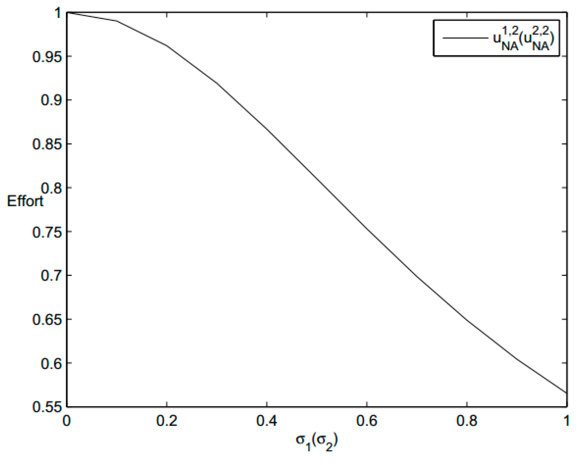
First, According Proposition 6, it is not difficult to find the relationship between the sales volume of the salesman ( u ) and the uncertain factors ( σ ). We have:
( u ¯ 1 , 1 u ¯ 1 , 2 u ¯ 2 , 1 u ¯ 2 , 2 ) = ( 2 σ 1 4 + 16 σ 1 2 + 16 3 σ 1 4 + 12 σ 1 2 + 8 σ 1 4 + 4 σ 1 2 + 8 3 σ 1 4 + 12 σ 1 2 + 8 2 σ 2 4 + 16 σ 2 2 + 16 3 σ 2 4 + 12 σ 2 2 + 8 σ 2 4 + 4 σ 2 2 + 8 3 σ 2 4 + 12 σ 2 2 + 8 )
The analytic result is borne out numerically. Figure 1 and Figure 2 respectively plot the relationship between the second-best efforts and σ 1 , σ 2 .
From above two figures, we see that the greater the impact of the uncertainty factor, the less effort the salesman provide. When the uncertainties tend to zero, the second-best effort tends to be the first-best effort. This conclusion is generally true, whether there is one salesman or multiple salesmen in the model. According to our assumptions, the first project is only affected by σ 1 , so when σ 1 = 0 , u S B 1 , 1 = u F B 1 , 1 and u S B 1 , 2 = u F B 1 , 2 are constants. Similarly, when σ 2 = 0 , u S B 2 , 1 = u F B 2 , 1 and u S B 2 , 2 = u F B 2 , 2 are constants.
Further, we describe the relationship between the second-best contract and gain-loss function. Fix the uncertainty with σ 1 = σ 2 = 1 and Y 0 1 = Y 0 2 = 0 . According (A15), we have
( Z 1 , 1 Z 1 , 2 Z 2 , 1 Z 2 , 2 ) = ( 17 23 13 23 17 23 13 23 )
obtaining that Φ ( Z ) = 0.9 . Substitute the above result into (A19), then we can get the result in Figure 3.
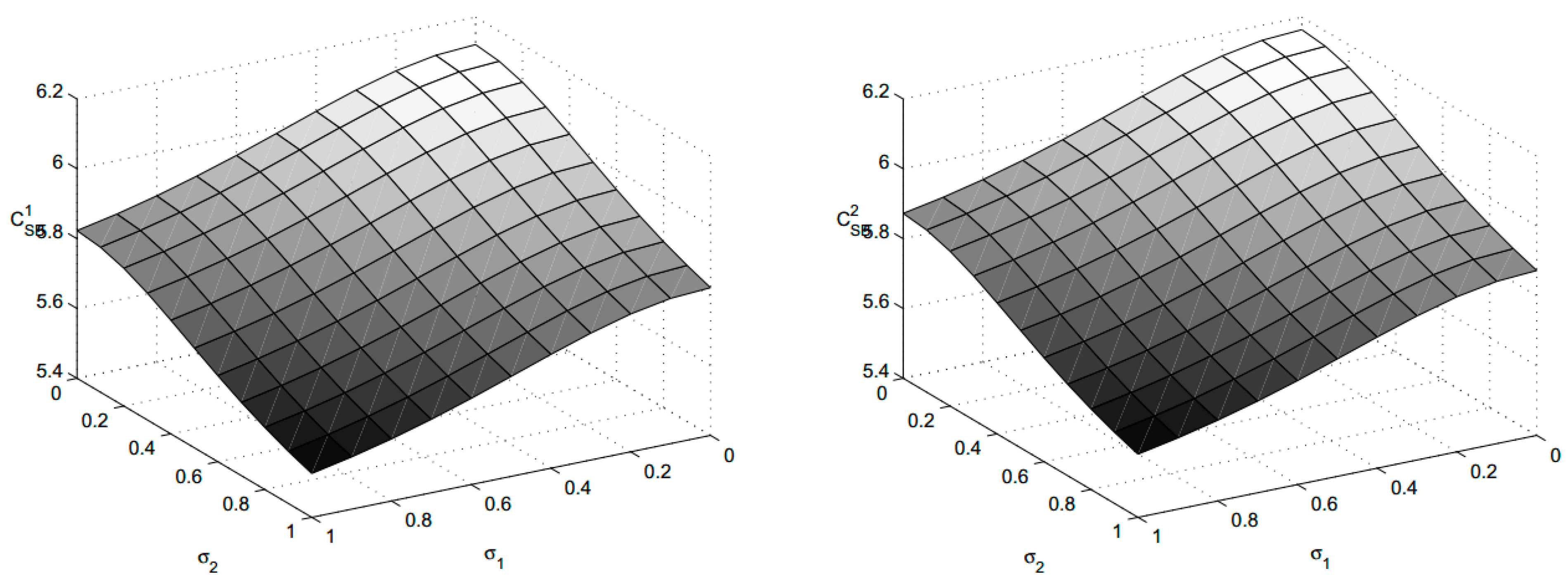
Figure 3 plots the second contract C S B 1 and C S B 2 , shows that C S B 1 and C S B 2 increases with the increase of λ . The greater the loss aversion coefficient λ , the greater the negative effect of wage gap on salesman Two, so the manager needs to offer a higher contract to motivate salesman Two to provide the recommended effort. According to our assumptions, we have calculated that C S B 1 C S B 2 . However, if λ is too large, there will be C S B 1 C S B 2 , then the wage gap would have a big negative effect on salesman One. Thus, for the manager, when the loss aversion coefficient is relatively large, the manager will provide two identical contracts to the salesmen to offset the gain-loss utility between salesman.
And we compare the impact on manager’s utility whether salesmen consider the gain-loss utility, and describe the relationship between the second-best contract and the uncertainties.
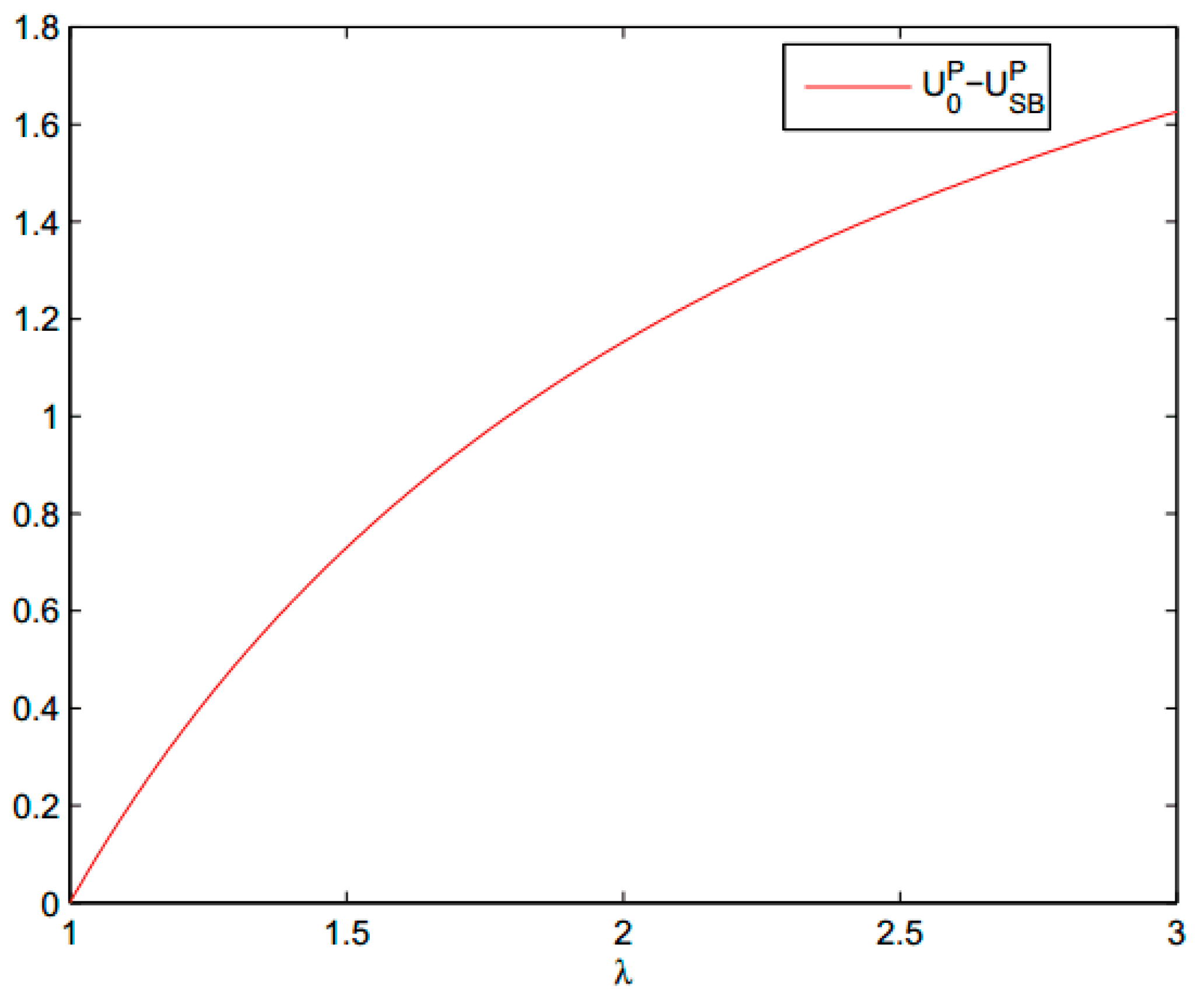
If salesmen do not consider the gain-loss utility, then for = 1 , 2 , V i ( C i , C i ) = 0 . Because ( X 0 1 , X 0 2 ) satisfies participation constraint, then e r 1 X 0 1 = e r 1 L 1 and e r 2 X 0 2 = e r 2 L 2 . Combined with the previous analysis results, we produce the result in Figure 4.
Figure 4 shows that U 0 P U S B P is non-negative that exactly reflect the conclusion of Proposition 8. When the loss aversion coefficient is larger, the larger contract the manager needs to be provided, but the optimal efforts are unchanged, then the manager’s utility will be lower.
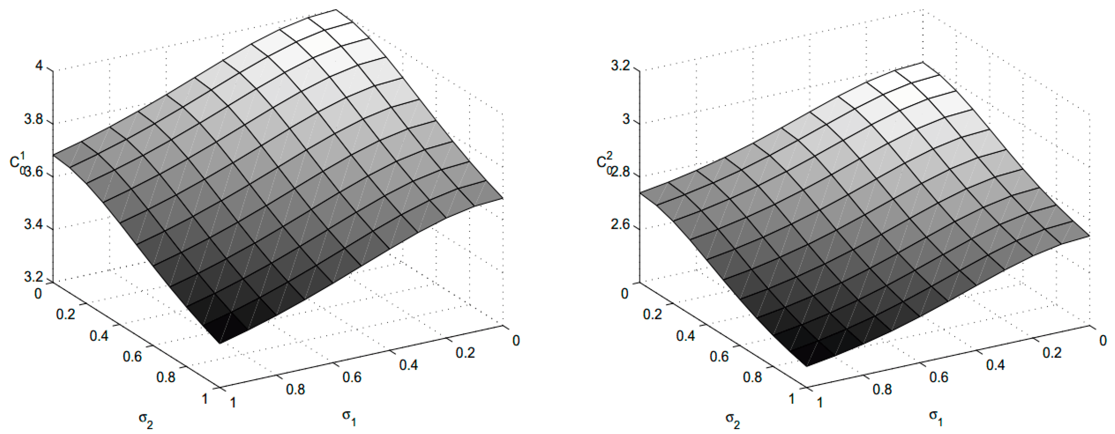
Figure 5 depicts the relationship between the second-best contract and uncertainty when the salesman does not consider the gain-loss utility.
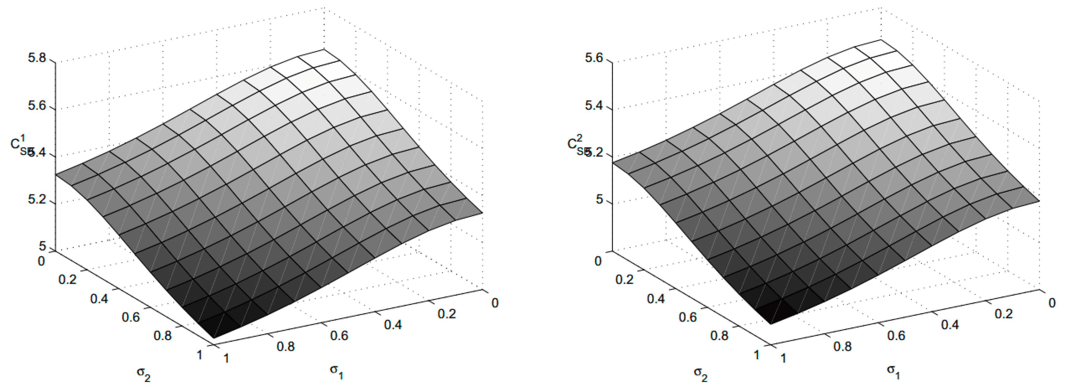
Figure 6 and Figure 7 describe the case where the second-best contract varies with σ 1 , σ 2 , where loss aversion coefficient λ = 1 and λ = 2 . The trend of the second-best contract in Figure 6 and 7 is similar to in Figure 5, because in all three cases, the greater uncertainty, the less effort the salesman provided, and therefore the smaller the contract the manager provided. In addition, it can be seen from the above three figures that as the loss avoidance coefficient increases, the second-best contract is also becoming larger and larger, which point to the conclusion of Figure 4.
According to the analysis of the above examples, we can see that: In addition to external uncertainties, the salesman’s behavior (or psychology) is another major factor affecting the expected utility of owner and salesman. In particular, when there is a vicious competition (or wage comparison) between salesmen, it will have a relatively large negative impact on sales. Therefore, how to promote the cooperation of salesman, and encourage them to work hard is a meaningful thing for owners.

5. Conclusions

In this paper, we extend the standard multiple agent problems in continuous time by adding personal loss aversion utility. After joining the personal loss aversion utility, each salesman uses his co-worker’s salary as his reference point. If his salary is higher than his co-worker’s, then the wage gap gives him positive utility; conversely, giving him negative utility. In our paper, we assume that the salesman’s material utility function and gain-loss function are separable and additive, refer to [17]. We cannot directly use the first-order method and the methods of BSDE to find the optimal contract. In some special cases, we are able to derive the explicit expressions of the optimal contract and the optimal effort.
Our research shows that incorporating behavioral preferences (the salesman’s concern about gains and losses) into contract theory is useful for studying the interactions between multiple salesmen. We show that the design of the optimal contract should not only consider the relationship of interest between manager and a salesman, but also pay attention to the factors of action between salesmen, such as the interaction between workers, the interest relations, etc. Our findings suggest that the second-best effort is less than the first-best effort, which is similar to the standard manager-salesman problem. The optimal effort is a decreasing function of uncertainty and the optimal contract is a linear function of the final asset.
Compared with the case of the salesmen without considering the gain-loss utility, the expected utility of the manager will be reduced if all salesmen consider the gain-loss utility. The salary of the high contract salesmen (paying more effort) is lower than the salesman without gain-loss utility, while the salary of the low contract salesman (who pay less effort) is more than the salary if he did not consider the gain-loss utility. This situation is somewhat similar to “winner curse”. For the high contract salesman, he wants to eliminate the gain-loss utility. For the manager, if one salesman considers the gain-loss utility, then the manager wishes another also would consider the gain-loss utility, but he still prefers that each salesman in the organization does not consider this utility. The other indicated point is that when the loss avoidance coefficient λ is relatively large, the manager will provide the same contract to each salesman, which is unfair to the salesman who pays more effort.
Our study provides a reference for further research on behavioral contract theory when the salesman’s utility function depends not only on his own salary level but also on the others. The model we build in this paper can be generalized to a more general multi-salesman model. In the future, we will make more research on the cooperative competition between salesmen, the fairness preference and so on.

Author Contributions

C.L. conceived and wrote the paper. S.-J.C. Revised the paper. P.-F.C. determined the content of the study, and directed the study.

Funding

This work was supported by the Key Projects of Hunan Social Science Achievement Evaluation Committee (Nos.XSP2016040508, XSP18ZD1002, XSP19ZDA009), the Human Philosophy Social Science Fund, projects (Nos.18YBA150, 13JD20), Key Project of Hunan Education Department (Nos. 18A201), Think Tank Project of Hunan Social Sciences Federation (Nos. ZK2019006), and Natural Science Foundations of Hunan (Nos. 2019JJ40088, 2019JJ40479).

Acknowledgments

The authors would like to express appreciation to the anonymous reviewers and editors for their very helpful comments on improving the paper, and all the people participated in the survey.

Conflicts of Interest

The authors declare no conflict of interest.

Appendix A

Appendix A.1

We define the gain-loss function of salesman i as follows
V i ( x ) = { e r i x + 1 if   x 0 , λ ( e r i x + 1 ) if   x 0 .
where x = C i C i , λ 1 . It is not difficult to verify that the gain-loss function satisfies the following conditions:
(I)
V i ( x ) , continuous for x , is second order differentiable when x 0 , and V i ( 0 ) = 0 .
(II)
V i ( x ) is strictly monotonous.
(III)
if 0 < x < y , then V i ( y ) + V i ( y ) V i ( x ) + V i ( x ) .
(IV)
If x > 0 , V i ( x ) 0 ; otherwise x < 0 , V i ( x ) 0 .
(V)
V i ( 0 ) V i + ( 0 ) λ , here V i + ( 0 ) lim x 0 + V i ( x ) , V i ( 0 ) lim x 0 V i ( x ) .
The gain-loss function in our paper is shown in Figure A1.
Figure A1. gain-loss function of salesman i .
Symmetry 11 00864 g0a1

Appendix B

Appendix B.1

Proof. 
Starting with maximization involves C . Because J is not a convex (or concave) function, the local maximum point may not be the global maximum point. To find global maximum of J on closed bound area, we should:
  • Find all local maximum points;
  • Find all non-differentiable points;
  • Find all max points on boundary;
  • Choose the biggest one, which is the global max point.
Since ρ i 0 , it can be clearly seen that J ( Y T , C , u t ) is continuous and second order differentiable. If J ( Y T , C ¯ , u t ) = ( J C 1 , J C 2 ) = 0 and 2 J ( Y T , C ¯ , u t ) < 0 , (Hessian matrix, negative definite matrix), then C ¯ is the local maximum point, and takes the first-order derivative of C i , then we let the derivative equal to zero:
i = 1 2 ρ i r i e r i ( C i G T i ) = 2 r P e r P ( Y T 1 + Y T 2 i = 1 2 C i )
Hence
C i = 1 r i ln ( ρ i r i r P ) + G T i + r P r i [ Y T 1 + Y T 2 ( C 1 + C 2 ) ]
together with:
C 1 + C 2 = 1 1 + r ¯ [ r ¯ ( Y T 1 + Y T 2 ) + G T 1 + G T 2 ] + 1 1 + r ¯ i = 1 2 1 r i ln ( ρ i r i r P )
where
r ¯ = ( r P r 1 + r P r 2 )
Therefore, an optimal contract C F B for Problem 1 as follows:
C F B i = 1 r i ln ( ρ i r i r P ) + G T i + r P r i ( 1 + r ¯ ) [ Y T 1 + Y T 2 + ( G T 1 + G T 2 ) + i = 1 2 1 r i ln ( ρ i r i r P ) ]
Next, we need to determine the Lagrange multipliers ρ i , and by Equation (A1), we know that Lagrange multipliers ρ 1 , ρ 2 > 0 . According to the Kuhn–Tucker condition, the salesman’s participation constraints are tight, namely
{ E u [ e r A 1 ( C 1 G T 1 ) e r A 1 ( C 1 C 2 ) + 1 ] = e r A 1 L 1 E u [ e r A 2 ( C 2 G T 2 ) + λ e r A 2 ( C 1 C 2 ) λ ] = e r A 2 L 2
Substitute Equation (A2) and Equation (A3) into Equation (A4), after a series of calculations, we finally have
{ e r P B 1 + r ¯ · x r 1 + r P 1 + r ¯ · y r P 1 + r ¯ e r 1 ( G 1 T G 2 T + D B ) · x r 1 ( 1 + D ) · y r 1 ( D 1 ) = e r 1 L 1 + 1 e r P B 1 + r ¯ · x r P 1 + r ¯ · y r 2 + r P 1 + r ¯ λ · e r 1 ( G 1 T G 2 T + D B ) · x r 2 ( 1 + D ) · y r 2 ( D 1 ) = e r 2 L 2 λ
where
{ x = exp ( 1 r 1 ln ( ρ 1 r 1 r P ) ) = ( r P ρ 1 r 1 ) 1 r 1 y = exp ( 1 r 2 ln ( ρ 2 r 2 r P ) ) = ( r P ρ 2 r 2 ) 1 r 2
and B Y T 1 + Y T 2 G T 1 G T 2 and D r P ( r 2 r 1 ) r 1 r 2 ( 1 + r ¯ ) .
Taking the derivative of manager’s utility with respect to u , the optimal effort u F B i is given by:
{ ( a 11 u 1 , 1 + a 12 u 1 , 2 ) | u 1 , 1 = g 1 , 1 | u 1 , 1 = k 1 u F B 1 , 1 ( a 11 u 1 , 1 + a 12 u 1 , 2 ) | u 1 , 2 = g 1 , 2 | u 1 , 2 = k 2 u F B 1 , 2 ( a 21 u 2 , 1 + a 22 u 2 , 2 ) | u 2 , 1 = g 2 , 1 | u 2 , 1 = k 1 u F B 2 , 1 ( a 21 u 1 , 1 + a 22 u 2 , 2 ) | u 2 , 2 = g 2 , 2 | u 2 , 2 = k 2 u F B 2 , 2
For finding all max points on boundary, we have C 2 [ 0 , C 1 ] and C 1 [ C 2 , Y T 1 + Y T 2 ] according to the assumptions. The payment C 1 can not be equal to 0 because the salesman has a reservation utility, thus the boundary point is C 1 = C 2 . Under the principal’s rational assumption, the salesman’s participation constraints are tight, namely:
{ E u 1 [ e r A 1 ( C 1 G T 1 ) ] = e r A 1 L 1 E u 2 [ e r A 2 ( C 2 G T 2 ) ] = e r A 2 L 2 { E u 1 [ e r A 1 ( C 1 G T 1 ) ] = e r A 1 L 1 E u 2 [ e r A 2 ( C 2 G T 2 ) ] = e r A 2 L 2
By Jensen’s inequality:
{ C 1 = L 1 + G T 1 C 2 = L 2 + G T 2
According to Equation (A7), plugging G T 1 , G T 2 back into Equation (A8), we obtain:
{ C 1 = L 1 + T ( a 11 2 + a 21 2 ) 2 k 1 C 2 = L 2 + T ( a 12 2 + a 22 2 ) 2 k 2
Given the parameters L i , k i , a i j , C 1 = C 2 is generally not established. Therefore, we can say that the global maximum point is not on the boundary. In other words, the local maximum point is the global maximum point. □

Appendix B.2

Proof. 
According to the proof in Appendix B.1, the salesmen have gain-loss utility. Their participation constraints (A4) are equivalent to
λ ( E u [ e r 1 ( C 1 G T 1 ) ] e r 1 L 1 ) = ( E u [ e r 2 ( C 2 G T 2 ) ] e r 2 L 2 )
where the salesmen are exactly the same and λ = 1 . We have:
C 1 G T 1 = C 2 G T 2
From Equation (A3) we can obtain that ρ 1 = ρ 2 . Through the salesman’s participation constraints, we can see
{ C F B 1 = G T 1 1 r 1 ln ( e r 1 L 1 + 1 e r 1 ( G T 1 G T 2 ) ) C F B 1 = G T 2 1 r 2 ln ( e r 2 L 2 1 + e r 2 ( G T 1 G T 2 ) )
where G T 1 = T ( a 11 2 + a 21 2 ) 2 k 1 and G T 2 = T ( a 12 2 + a 22 2 ) 2 k 2 .
Next, we compare the expected utility of the manager when the salesman has or does not have gain-loss utility. When under the condition that the salesman has no gain-loss utility, the salesman’s participation constraints are as follows:
{ E u 1 [ e r A 1 ( C 1 G T 1 ) ] = e r A 1 L 1 E u 2 [ e r A 2 ( C 2 G T 2 ) ] = e r A 2 L 2
According to our assumption C F B 1 > C F B 2 with combining equation set (A4), we know that
{ C F B 1 L 1 + G T 1 = C ¯ 1 C F B 2 L 2 + G T 2 = C ¯ 2
Let C F B 1 + c 1 = C ¯ 1 and C F B 2 c 2 = C ¯ 2 ( c 1 , c 2 0 ), substitute it into Equation (A9), then
2 = e r 1 c 1 + e r 2 c 2 2 e r 1 c 1 e r 2 c 2 , r 1 = r 2
hence, we say c 1 c 2 , namely, C F B 1 + C F B 2 C ¯ 1 + C ¯ 2 . Under symmetric information, the optimal effort of salesman is invariable no matter the salesman has or has no gain-loss utility. Thus:
U P ( Y T , C ) U 0 P ( Y T , C )
 □

Appendix C

Appendix C.1

Before proving Proposition 3, we first give a lemma.
Assumption A1.
For any ( t , y , z ) [ 0 , T ] × R m × R m × d , the map g : [ 0 , T ] × R m × R m × d R m is R m - valued and F -predictable process, and satisfied
0 T | g ( · , 0 , 0 ) | 2 d t < ,
and moreover, g about ( y , z ) satisfies Lipschitz condition: for some constant K > 0 and y , y R m , z , z R m × d , such that
| g ( t , y , z ) g ( t , y , z ) | K ( | y y | + | z z | ) .
Lemma A1.
If g satisfied Assumption 1, for any given terminal condition ξ is Lebesgue square measurable, a BSDE is given by
Y t = ξ + t T g ( s , y , z ) d s t T Z s d B s
which has a unique solution.
Proof This Lemma is Proposition 2.2 in Yan et al. [29].
Proof of Proposition 3.
Sufficiency: By definition of Nash equilibrium effort, u ¯ i is the optimal effort for salesman i , which means that:
U 0 i ( C i , C i , u ¯ i , u ¯ i ) = E u ¯ i , u ¯ i [ e r i ( C i 0 T g i ( u ¯ i ) d t ) + V i ( C i , C i ) ] = sup u i A i   E u i , u ¯ i [ e r i ( C i 0 T g i ( u i ) d t ) + V i ( C i , C i ) ]
Denoting that U ˜ s i ( C i , C i , u i , u i ) = U s i ( C i , C i , u i , u i ) V i ( C i ) , for i = 1 , , N , we know that U ˜ s i ( C i , C i , u i , u i ) < 0 .
U 0 i ( C i , C i , u ¯ i , u ¯ i ) U 0 i ( C i , C i , u i , u ¯ i ) = t T r i [ U s i ( C i , C i , u ¯ i , u ¯ i ) U s i ( C i , C i , u i , u ¯ i ) ] Z s i Σ s d B s t T r i U ˜ s i ( C i , C i , u ¯ i , u ¯ i ) · Z s i · b ( s , A , u ¯ s i , u ¯ s i ) g i ( u ¯ s i ) ) d s + t T r i U ˜ s i ( C i , C i , u i , u ¯ i ) · Z s i · b ( s , A , u ¯ s i , u ¯ s i ) g i ( u s i ) ) d s t T r i [ U s i ( C i , C i , u ¯ i , u ¯ i ) U s i ( C i , C i , u i , u ¯ i ) ] Z s i Σ s d B s t T r i U ˜ s i ( C i , C i , u i , u ¯ i ) [ Z s i · b ( s , A , u ¯ s i , u ¯ s i ) g i ( u ¯ s i ) ( Z s i · b ( s , A , u s i , u ¯ s i ) g i ( u s i ) ) ] d s
Because U 0 i ( C i , C i , u ¯ i , u ¯ i ) U 0 i ( C i , C i , u i , u ¯ i ) , taking the expectation, the inequality still holds. This implies that for any u i A i , i = 1 , , N , we have:
Z s i · b ( s , A , u ¯ s i , u ¯ s i ) g i ( u ¯ s i ) Z s i · b ( s , A , u s i , u ¯ s i ) g i ( u s i )
In other words,
u ¯ s i sup u s i A i { Z s i · b ( s , A , u s i , u ¯ s i ) g i ( u s i ) }
as a function f i , u i we defined in Section 4:
f i , u i ( · , Z i ) = r i 2 Z i Σ 2 + sup u i A i { Z i · b ( · , A , u i , u ¯ i ) g i ( u i ) }
For any ( t , ω , z ) [ 0 , T ] × Ω × R 2 , the map f i , u i : [ 0 , T ] × Ω × R N R is R N - valued and F -predictable process, satisfies:
0 T | f i , u i ( · , 0 ) | d s L 2 ( Ω , F T , , R )
According to our setting, obviously, for some constant > 0 , there is b ( · , A , u ) K ( 1 + u ) and lim u i + | g i ( u i ) | | u i | = lim u i + k i u i 2 2 u i + , | g i ( u i ) | = | k i u i 2 2 | K ( 1 + u i 2 ) . Then, base on Lemma 4.1 in [25], for some contract K > 0 , we have
| f i , u i ( s , Z i ) | K ( 1 + Z s i 2 )
f i , u i ( s , Z s i ) satisfies Lemma 1. Hence, BSDE (7) has a unique solution.
Necessity: We assume that ( X ^ i , Z ^ i ) is a solution for BSDE (7), namely:
X ^ t i = C i + t T [ r i 2 Z ^ s i Σ s 2 + sup u i A i { Z ^ s i · b ( s , A , u s ) g i ( u s i ) } ] d s t T Z ^ s i Σ s d B s
From the uniqueness of ( X ^ i , Z ^ i ) , Z ^ i · b ( · , A , u i , u i ) g i ( u i ) is quadratic linearity about u i . Hence, we can say there exists a effort process u ¯ s i , i = 1 , , N , such that:
u ¯ s i = sup u s i A i { Z ^ i · b ( s , A , u s i , u s i ) g i ( u s i ) } s [ t , T ]
Next, we prove u ¯ i is an optimal effort for salesman i . For u - i A i and given Z ^ i :
X ^ - 0 i = C i + 0 T [ r i 2 Z ^ s i Σ s 2 + { Z ^ s i · b ( s , A , u - s i , u s i ) g i ( u - s i ) } ] d s 0 T Z ^ s i Σ s d B s X ^ 0 i
According to Equation (A6),
U 0 i ( C i , C i , u i , u i ) V i ( C i , C i ) = e r i X 0 i
then we have
U 0 i ( C i , C i , u ¯ i , u i ) U 0 i ( C i , C i , u - i , u i )
for u - i A i , we confirm that u ¯ i is a optimal effort for salesman i . □

Appendix C.2

Proof. 
Recall that:
u ¯ = ( u ¯ 1 , 1 u ¯ 1 , N u ¯ N , 1 u ¯ N , N ) = ( a 11 k 1 Z 1 , 1 a 1 N k N Z 1 , N a N 1 k 1 Z N , 1 a N N k N Z N , N )
Therefore, we have
b ( t , A , u ¯ t ) = ( a 11 2 k 1 Z t 1 , 1 + + a 1 N 2 k N Z t 1 , N a N 1 2 k 1 Z t N , 1 + + a N N 2 k N Z t N , N )
And
f u ¯ ( t , Z ) = ( f 1 , u ¯ 1 ( t , Z ) f N , u ¯ N ( t , Z ) ) = ( r 1 2 · i = 1 N [ j = 1 N ( Z j , 1 σ j i ) 2 ] r N 2 · i = 1 N [ j = 1 N ( Z j , N σ j i ) 2 ] ) + ( j = 1 N [ Z j , 1 · ( i = 1 N a j i 2 k i Z j , i ) ] j = 1 N [ Z j , N · ( i = 1 N a j i 2 k i Z j , i ) ] ) ( j = 1 N ( a j 1 Z j , 1 ) 2 2 k 1 j = 1 N ( a j N Z j , N ) 2 2 k N )
Σ Σ = ( j = 1 N σ 1 j 2 j = 1 N σ 1 j σ 2 j j = 1 N σ 1 j σ N j j = 1 N σ 1 j σ 2 j j = 1 N σ 2 j 2 j = 1 N σ 2 j σ N j j = 1 N σ 1 j σ N j j = 1 N σ 2 j σ N j j = 1 N σ N j 2 ) ( m 11 m 21 m N 1 m 12 m 22 m N 2 m 1 N m 2 N m N N )
Thus b ( t , A , u ¯ t ) = j = 1 N ( i = 1 N a j i 2 k i Z t j , i ) ,
f u ¯ ( t , Z ) = l = 1 N { r l 2 · i = 1 N [ ( j = 1 N Z j , l σ j i ) 2 ] + j = 1 N ( a j l Z j , l ) 2 2 k l } + l = 1 N { j = 1 N [ Z j , l · ( i = 1 N a j i 2 k i Z j , i ) ] }
The HJB equation can be written as:
0 = t v + sup z Z ( R N ) { y v · b ( t , A , u ¯ t ) + x v · z · b ( t , A , u ¯ t ) f u ¯ ( t , z ) + 1 2 Tr ( Σ Σ · y y v ) + 1 2 Tr ( z Σ ( z Σ ) · x x v ) + Tr ( Σ Σ z · x y v ) }
According to the form of terminal condition, we assume that at any time t, the solution of HJB equation has the following form. For some function φ ( t ) , we have
v ( t , y , x ) = φ ( t ) e r P ( y x )
Then
t v = φ ( t ) φ ( t ) v y v = r P v x v = r P v y y v = r P 2 v x y v = r P 2 v x x v = r P 2 v
furthermore, we have:
{ Tr ( Σ Σ · y y v ) = r P 2 · v · j = 1 N ( i = 1 N σ j i 2 ) Tr ( Σ Σ Z · x y v ) = r P 2 · v · i = 1 N [ j = 1 N ( l = 1 N m j l ) · Z j , l ] Tr ( Z Σ Σ Z · x x v ) = r P 2 · v · [ j , k = 1 N ( j , l = 1 N m j k · Z j , i · Z k , l ) ]
Based on the above analysis, it is not difficult to see that HJB equation is a quadratic linear equation concerning the control variable Z j , i ( i , j = 1 , , N ). Fixed other parameters, if we take the first order condition for Z j , i , then we have:
{ r i · [ ( l = 1 N σ j l 2 ) · Z j , i + k = 1 , k j N ( l = 1 N σ j l σ k l Z k , i ) ] + a j i 2 k i Z j , i }    a j i 2 k i + r P · [ m j j Z j , i + k = 1 N ( l = 1 , ( k , l ) ( j , i ) N m j k Z k , l ) ] r P · l = 1 N m j l = 0
That is, for j = 1 , 2 , , N , Z j , i satisfies the following linear equations:
r P · l = 1 N m j l + a j i 2 k 1 = r P · k = 1 N ( l = 1 , ( k , l ) ( j , 1 ) N m j l Z k , l ) + r 1 · k = 1 , k j N ( m j , k Z k , 1 ) + { [ r N · ( l = 1 N σ j l 2 ) + a j 1 2 k 1 + r P · m j j } · Z j , 1 r P · l = 1 N m j l + a j N 2 k N = r P · k = 1 N ( l = 1 , ( k , l ) ( j , N ) N m j k Z k , l ) + r N · k = 1 , k j N ( m j , k Z k , N ) + { [ r N · ( l = 1 N σ j l 2 ) + a j N 2 k N + r P · m j j } · Z j , N
By solving this system of linear equations, we can obtain the explicit solution of the optimal control variable Z j , i ( i = 1 , 2 , , N ):
( Z N A 1 , 1 Z N A 1 , N Z 2 , 1 Z 2 , N Z N , 1 Z N A N , N ) = ( m 1 , 1 m 1 , N m 1 , N + 1 m 1 , N × N m N , 1 m N , N m N , N + 1 m N , N × N m N + 1 , 1 m N + 1 , N m N + 1 , N + 1 m N + 1 , N × N m N × N , 1 m N × N , N m N × N , N + 1 m N × N , N × N ) 1 · ( r P · l = 1 N m 1 l + a 11 2 k 1 r P · l = 1 N m 1 l + a 1 N 2 k N r P · l = 1 N m 2 l + a 21 2 k 1 r P · l = 1 N m 2 l + a 2 N 2 k N r P · l = 1 N m N l + a N 1 2 k 1 r P · l = 1 N m N l + a N N 2 k N )
here, for j , i , l = 1 , 2 , , N
when ( j 1 ) × N < τ j × N m τ , τ = [ r i · ( l = 1 N σ j l 2 ) + a j i 2 k i ] + r P · m j j
when ( j 1 ) × N < τ j × N , ( l 1 ) × N < κ l × N m τ , κ = { ( r P + r i ) · m j l , κ = ( l 1 ) × N + i r P · m j l ,     κ ( l 1 ) × N + i
The Proposition 5 is proved. □

Appendix C.3

Proof. 
Under the assumptions that: i , j = 1 , 2 , a i j = a , r i = r , σ j j = σ j , m j j = σ j 2 , and m 12 = m 21 = 0 , by substituting the above parameters into Equation (A12) of Proposition 5, we have:
( Z 1 , 1 Z 1 , 2 Z 2 , 1 Z 2 , 2 ) = ( ( r P + r ) σ 1 2 + a 2 k 1 r P σ 1 2 0 0 r P σ 1 2 ( r P + r ) σ 1 2 + a 2 k 2 0 0 0 0 ( r P + r ) σ 2 2 + a 2 k 1 r P σ 2 2 0 0 r P σ 2 2 ( r P + r ) σ 2 2 + a 2 k 2 ) 1 · ( r P σ 1 2 + a 2 k 1 r P σ 1 2 + a 2 k 2 r P σ 2 2 + a 2 k 1 r P σ 2 2 + a 2 k 2 )
Denote that
Λ 1 = ( ( r P + r ) σ 1 2 + a 2 k 1 r P σ 1 2 r P σ 1 2 ( r P + r ) σ 1 2 + a 2 k 2 ) Λ 2 = ( ( r P + r ) σ 2 2 + a 2 k 1 r P σ 2 2 r P σ 2 2 ( r P + r ) σ 2 2 + a 2 k 2 ) Λ 3 = ( r P σ 1 2 + a 2 k 1 r P σ 1 2 + a 2 k 2 )    Λ 4 = ( r P σ 2 2 + a 2 k 1 r P σ 2 2 + a 2 k 2 )
Then
( Z 1 , 1 Z 1 , 2 Z 2 , 1 Z 2 , 2 ) = ( Λ 1 1 0 0 Λ 2 1 ) · ( Λ 3 Λ 4 )
We next prove that the second-best effort is less than the first-best effort. Obviously, we only need to prove Z i , j 1 to hold the conclusion. For proving Z i , j 1 , according to Equation (A15), we can easily calculate that:
Z 1 , 1 = [ ( r P + r 1 ) σ 1 2 + a 2 k 2 ] · ( r P σ 1 2 + a 2 k 1 ) r P σ 1 2 · ( r P σ 1 2 + a 2 k 2 ) [ ( r P + r 1 ) σ 1 2 + a 2 k 1 ] · [ ( r P + r 1 ) σ 1 2 + a 2 k 2 ] ( r P σ 1 2 ) 2
Obviously:
[ ( r P + r 1 ) σ 1 2 + a 2 k 2 ] · [ ( ( r P + r 1 ) σ 1 2 + a 2 k 1 ) ( r P σ 1 2 + a 2 k 1 ) ] + r P σ 1 2 · [ r P σ 1 2 + a 2 k 2 r P σ 1 2 ] 0
Therefore, Z 1 , 1 1 . When σ 1 = 0 , we have Z 1 , 1 = 1 .
Similarly, we can prove that Z 1 , 2 1 , Z 2 , 1 1 and Z 2 , 2 1 . □

Appendix C.4

Proof. 
According to Proposition 4, we have
C S B i = X 0 i 0 T ( r i 2 Z s i Σ s 2 + Z s i b ( s , A , f i ( Z s i ) ) k i f i ( Z s i ) 2 2 ) d s + 0 T Z s i Σ s d B s = X 0 i 0 T ( r i 2 Z s i Σ s 2 + Z s i b ( s , A , f i ( Z s i ) ) k i f i ( Z s i ) 2 2 ) d s + 0 T Z s i d Y s
Then
C S B i = X 0 1 T Z 1 , 1 ( a 2 k 1 Z 1 , 1 + a 2 k 2 Z 1 , 2 ) T Z 2 , 1 ( a 2 k 1 Z 2 , 1 + a 2 k 2 Z 2 , 2 ) + Z 1 , 1 Y T 1 + Z 2 , 1 Y T 2 + a 2 T 2 k 1 [ ( Z 1 , 1 ) 2 + ( Z 2 , 1 ) 2 ] + r T 2 [ ( σ 11 Z 1 , 1 + σ 21 Z 2 , 1 ) 2 + ( σ 12 Z 1 , 1 + σ 22 Z 2 , 1 ) 2 ] C S B 2 = X 0 2 T Z 1 , 2 ( a 2 k 1 Z 1 , 1 + a 2 k 2 Z 1 , 2 ) T Z 2 , 2 ( a 2 k 1 Z 2 , 1 + a 2 k 2 Z 2 , 2 ) + Z 1 , 2 Y T 1 + Z 2 , 2 Y T 2 + a 2 T 2 k 2 [ ( Z 1 , 2 ) 2 + ( Z 2 , 2 ) 2 ] + r T 2 [ ( σ 11 Z 1 , 2 + σ 21 Z 2 , 2 ) 2 + ( σ 12 Z 1 , 2 + σ 22 Z 2 , 2 ) 2 ]
Therefore,
C S B 1 C S B 2 = X 0 1 X 0 2 + Φ ( Z )
Here
Φ ( Z ) = T [ ( a 2 k 2 ( Z 1 , 2 ) 2 + ( Z 2 , 2 ) 2 ) ] T [ ( a 2 k 1 ( Z 1 , 1 ) 2 + ( Z 2 , 1 ) 2 ) ] + ( a 2 k 1 a 2 k 2 ) · ( Z 1 , 1 Z 1 , 2 + Z 2 , 1 Z 2 , 2 ) + ( Z 1 , 1 Z 1 , 2 ) Y T 1 + ( Z 2 , 1 Z 2 , 2 ) Y T 2 + a 2 T 2 k 1 [ ( Z 1 , 1 ) 2 + ( Z 2 , 1 ) 2 ] a 2 T 2 k 2 [ ( Z 1 , 2 ) 2 + ( Z 2 , 2 ) 2 ] + r T 2 [ ( σ 11 Z 1 , 1 + σ 21 Z 2 , 1 ( 2 + ( σ 12 Z 1 , 1 + σ 22 Z 2 , 1 ) 2 ] ( σ 11 Z 1 , 2 + σ 21 Z 2 , 2 ) 2 ( σ 12 Z 1 , 2 + σ 21 Z 2 , 2 ) 2 ]
Substituting Equation (A16) into the participation constraints of salesman, then:
{ e r X 0 1 + ( e r ( X 0 1 X 0 2 + Φ ( Z ) ) + 1 ) = e r L e r X 0 2 λ ( e r ( X 0 1 X 0 2 + Φ ( Z ) ) + 1 ) = e r L
Then we get:
{ e r X 0 1 = ( 1 + 1 λ ) e r L e r X 0 2 e r X 0 2 = ( e r Φ ( Z ) + 1 1 λ e r L ) + ( e r Φ ( Z ) + 1 1 λ e r L ) 2 + 4 ( 1 + 1 λ ) e r ( Φ ( Z ) + L ) 2 ( 1 + 1 λ ) e r ( Φ ( Z ) + L )
 □

Appendix C.5

Proof. 
From Proposition 5, we know that the second-best effort for two salesmen is constants regardless of whether the salesmen consider gain-loss utility. So, in both cases, the final output Y T is the same. We set U 0 P ( Y T , C ¯ S B ) to represent the manager’s utility when the salesmen do not consider gain-loss utility, where C ¯ S B represents the second-best contract in this case, and U S B P ( Y T , C S B ) represents the manager’s utility when the salesmen consider gain-loss utility, where C S B represents the second-best contract in this case. Hence:
U 0 P ( Y T , C ¯ S B ) = e r P ( Y T 1 + Y T 2 C ¯ S B 1 C ¯ S B 2 ) U S B P ( Y T , C S B ) = e r P ( Y T 1 + Y T 2 C S B 1 C S B 2 )
According to participation constraints (A18), we can get X ¯ 0 1 = X ¯ 0 2 = L when the salesmen are no consider gain-loss utility. Therefore, on the basis of Proposition 7, we only need to prove that ( X 0 1 + X 0 2 ) ( X ¯ 0 1 + X ¯ 0 2 ) = 2 L , and then certify U 0 P ( Y T , C ¯ S B ) U S B P ( Y T , C S B ) . By Equation (A19):
e r X 0 1 + e r X 0 2 = ( 1 + 1 λ ) e r L 2 e r 2 ( X 0 1 + X 0 2 ) ( 1 + 1 λ ) e r L e r ( X 0 1 + X 0 2 ) 2 λ 1 + λ e r ( X 0 1 + X 0 2 ) e 2 r L 2 r L r ( X 0 1 + X 0 2 ) ( X ¯ 0 1 + X ¯ 0 2 ) = 2 L ( X 0 1 + X 0 2 )
Finally, U 0 P ( Y T , C ¯ S B ) U S B P ( Y T , C S B ) is proved and the Proposition is established. □

References

  1. Lal, R.; Srinivasan, V. Compensation plans for single-and multi-product salesforces: An application of the Holmstrom-Milgrom model. Manag. Sci. 1993, 39, 777–793. [Google Scholar] [CrossRef]
  2. Chan, T.-Y.; Li, J.; Pierce, L. Compensation and peer effects in competing sales teams. Manag. Sci. 2014, 60, 1965–1984. [Google Scholar] [CrossRef]
  3. Chung, J.; Narayandas, D. Incentives versus reciprocity: Insights from a field experiment. J. Mark. Res. 2017, 54, 511–524. [Google Scholar] [CrossRef]
  4. Basu, A.; Lal, R.; Srinivasan, V.; Staelin, R. Salesforce compensation plans: An agency theoretic perspective. Mark. Sci. 1985, 4, 267–291. [Google Scholar] [CrossRef]
  5. Coughlan, A.; Narasimhan, C. An empirical analysis of sales-force compensation plans. J. Bus. 1992, 65, 93–121. [Google Scholar] [CrossRef]
  6. Chen, F. Salesforce incentives, market information, and production/inventory planning. Manag. Sci. 2005, 51, 60–75. [Google Scholar] [CrossRef]
  7. Rubel, O.; Prasad, A. Dynamic incentives in sales force compensation. Mark. Sci. 2015, 35, 676–689. [Google Scholar] [CrossRef]
  8. Kräkel, M.; Schöttner, A. Optimal sales force compensation. J. Econ. Behav. Organ. 2016, 126, 179–195. [Google Scholar] [CrossRef] [Green Version]
  9. Albers, S. Optimization models for salesforce compensation. Eur. J. Oper. Res. 1996, 89, 1–17. [Google Scholar] [CrossRef]
  10. Rouziès, D.; Coughlan, A.; Anderson, E.; Iacobucci, D. Determinants of pay levels and structures in sales organizations. J. Mark. 2009, 73, 92–104. [Google Scholar]
  11. Bommaraju, R.; Hohenberg, S. Self-Selected Sales Incentives: Evidence of their Effectiveness, Persistence, Durability, and Underlying Mechanisms. J. Mark. 2018, 82, 106–124. [Google Scholar] [CrossRef]
  12. Holmstrom, B. Moral hazard in teams. Bell J. Econ. 1982, 13, 324–340. [Google Scholar] [CrossRef]
  13. McAfee, R.; McMillan, J. Competition for agency contracts. RAND J. Econ. 1987, 18, 296–307. [Google Scholar] [CrossRef]
  14. Itoh, H. Incentives to help in multi-agent situations. Econometrica 1991, 59, 611–636. [Google Scholar] [CrossRef]
  15. Tian, H.-P.; Liu, C.-X.; Guo, Y.-J. Pay scheme designing method with multiple agents’ competition. J. Ind. Eng. Eng. Manag. 2007, 21, 153–156. [Google Scholar]
  16. Caldieraro, F.; Coughlan, A. Optimal sales force diversification and group incentive payments. Mark. Sci. 2009, 28, 1009–1026. [Google Scholar] [CrossRef]
  17. K˝oszegi, B.; Rabin, M. A model of reference-dependent preferences. Q. J. Econ. 2006, 121, 1133–1165. [Google Scholar]
  18. K˝oszegi, B.; Rabin, M. Reference-dependent risk attitudes. Am. Econ. Rev. 2007, 97, 1047–1073. [Google Scholar] [CrossRef]
  19. K˝oszegi, B.; Rabin, M. Reference-dependent consumption plans. Am. Econ. Rev. 2009, 99, 909–936. [Google Scholar] [CrossRef]
  20. Herweg, F.; Müller, D.; Weinschenk, P. Binary Payment Schemes: Moral Hazard and Loss Aversion. Am. Econ. Rev. 2010, 100, 2451–2477. [Google Scholar] [CrossRef]
  21. Dittmann, I.; Maug, E.; Spalt, O. Sticks or Carrots? Optimal CEO Compensation when Managers Are Loss Averse. J. Financ. 2010, 65, 2015–2050. [Google Scholar] [CrossRef] [Green Version]
  22. Daido, K.; Murooka, T. Team Incentives and Reference-Dependent Preferences. J. Econ. Manag. Strat. 2016, 25, 958–989. [Google Scholar] [CrossRef]
  23. Goukasian, L.; Wan, X.-H. Optimal incentive contracts under relative income concerns. Math. Financ. Econ. 2010, 4, 57–86. [Google Scholar] [CrossRef] [Green Version]
  24. Elie, R.; Mastrolia, T.; Possamaï, D. A Tale of a Principal and Many, Many Agents. Math. Oper. Res. 2018. [Google Scholar] [CrossRef]
  25. Elie, R.; Possamaï, D. Contracting theory with competitive interacting agents. SIAM J. Control Optim. 2019, 57, 1157–1188. [Google Scholar] [CrossRef]
  26. Kahneman, D.; Tversky, A. Prospect Theory: An Analysis of Decision under Risk. Econometrica 1979, 47, 263–291. [Google Scholar] [CrossRef]
  27. Cvitani’c, J.; Possamaï, D.; Touzi, N. Dynamic programming approach to principal-agent problems. Financ. Stoch. 2018, 22, 1–37. [Google Scholar] [CrossRef]
  28. Keun Koo, H.; Shim, G.; Sung, J. Optimal Multi-Agent Performance Measures for Team Contracts. Math. Financ. 2008, 18, 649–667. [Google Scholar] [CrossRef]
  29. Yan, J.-A.; Peng, S.-G.; Fang, S.-Z.; Wu, L.-M. Stochastic Analysis; Science Press: Beijing, China, 1997. [Google Scholar]
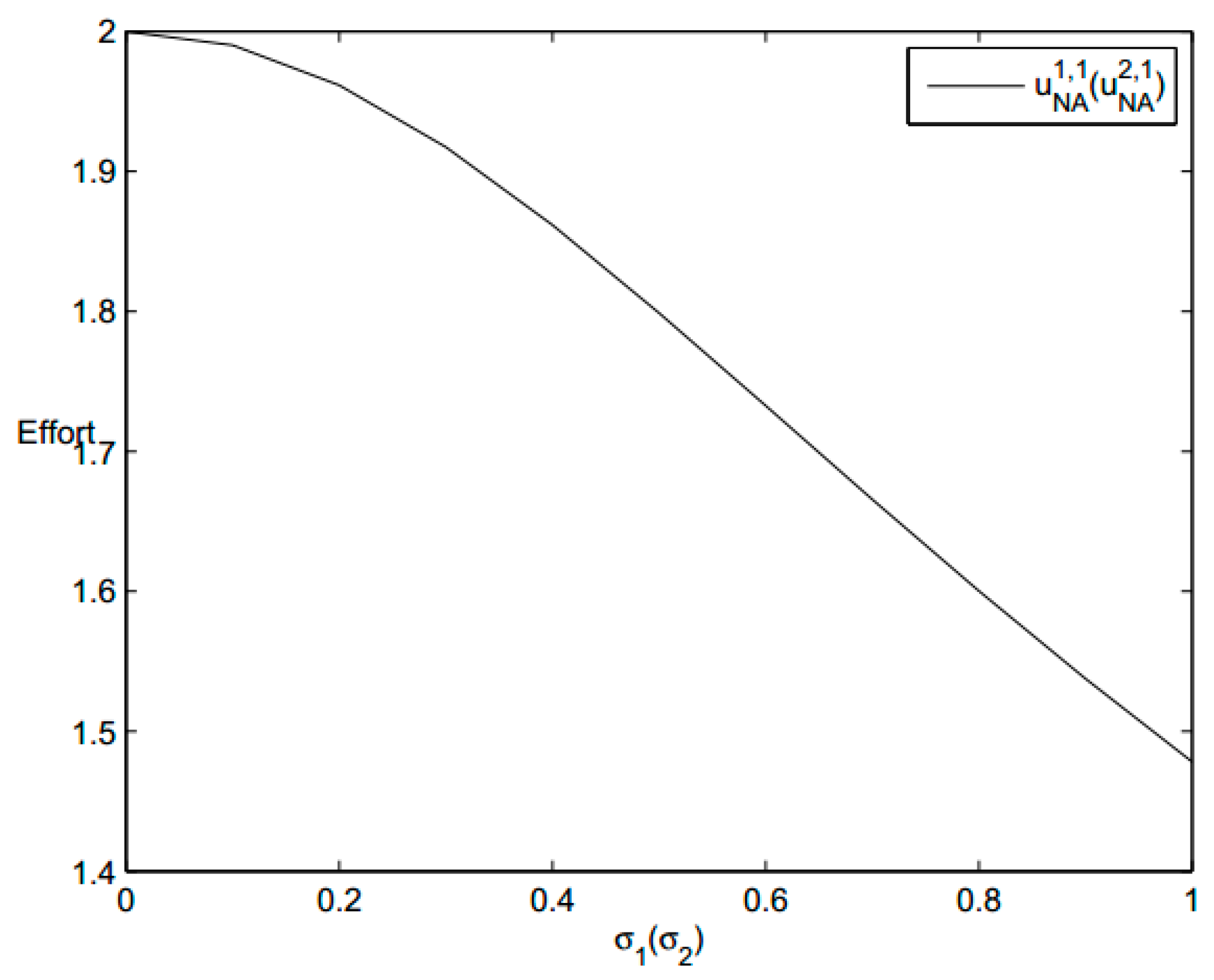
Figure 1. Salesman One’s second-best effort for different noise levels σ i .
Symmetry 11 00864 g001
Figure 2. The salesman Two’s second-best effort for different noise levels σ i .
Symmetry 11 00864 g002
Figure 3. The second-best contract for different λ .
Symmetry 11 00864 g003
Figure 4. The trend of U 0 P U S B P under different loss aversion coefficient λ .
Symmetry 11 00864 g004
Figure 5. The second-best contract under no consider the gain-loss utility.
Symmetry 11 00864 g005
Figure 6. The second-best contract under λ = 1 .
Symmetry 11 00864 g006
Figure 7. second-best contract under λ = 2 .
Symmetry 11 00864 g007

Share and Cite

MDPI and ACS Style

Li, C.; Cheng, S.-J.; Cheng, P.-F. Optimal Incentive Contract for Sales Team with Loss Aversion Preference. Symmetry 2019, 11, 864. https://doi.org/10.3390/sym11070864

AMA Style

Li C, Cheng S-J, Cheng P-F. Optimal Incentive Contract for Sales Team with Loss Aversion Preference. Symmetry. 2019; 11(7):864. https://doi.org/10.3390/sym11070864

Chicago/Turabian Style

Li, Chao, Si-Jie Cheng, and Peng-Fei Cheng. 2019. "Optimal Incentive Contract for Sales Team with Loss Aversion Preference" Symmetry 11, no. 7: 864. https://doi.org/10.3390/sym11070864

APA Style

Li, C., Cheng, S. -J., & Cheng, P. -F. (2019). Optimal Incentive Contract for Sales Team with Loss Aversion Preference. Symmetry, 11(7), 864. https://doi.org/10.3390/sym11070864

Note that from the first issue of 2016, this journal uses article numbers instead of page numbers. See further details here.

Article Metrics