Accelerating Density Peak Clustering Algorithm


Abstract
1. Introduction
2. Related Works
2.1. Clustering Methods
2.2. Density Peak Clustering Algorithm
| Algorithm 1. DPC algorithm. |
| Input: the set of data points and the parameters for defining the neighborhood, and for selecting density peaks |
| Output: the label vector of cluster index |
Algorithm:
|
3. Accelerating APC by Scanning Neighbors Only
| Algorithm 2. ADPC1 algorithm. |
| Input: the set of data points and the parameters for defining the neighborhood, and for selecting density peaks. |
| Output: the label vector of cluster index |
Algorithm:
|
4. Accelerating APC by Skipping Non-Peaks
| Algorithm 3. ADPC2 algorithm. |
| Input: the set of data points and the parameters for defining the neighborhood, and for selecting density peaks |
| Output: the label vector of cluster index |
Algorithm:
|
5. Performance Study
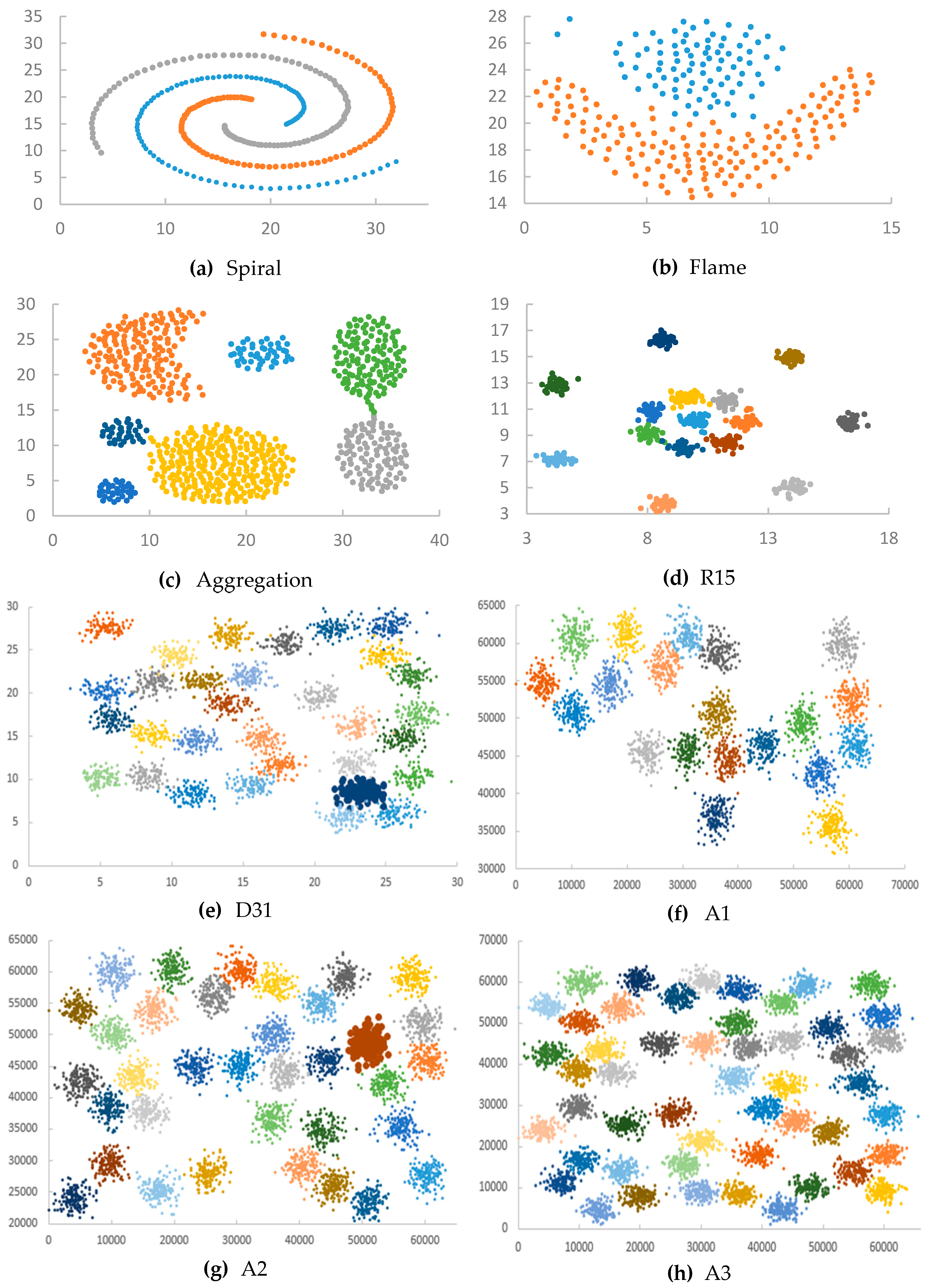
5.1. Test Datasets
5.2. Experiment Setup
5.3. Experiment Results
5.3.1. Test 1: Use a Fixed Threshold for Local Density
5.3.2. Test 2: Use an Exponential Kernel for Local Density
6. Conclusions
Funding
Acknowledgments
Conflicts of Interest
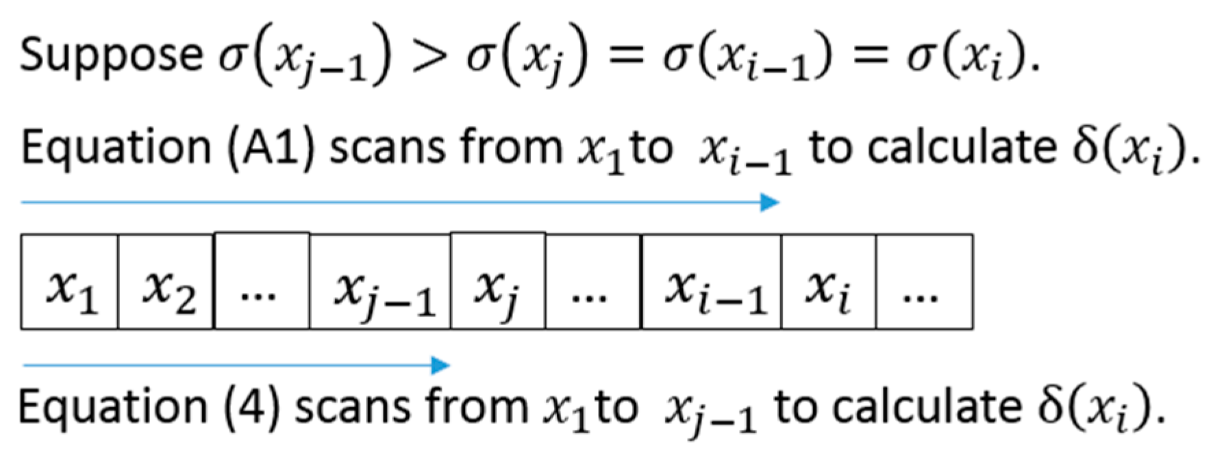
Appendix A. Implementation Details for Calculating Separation Distance in DPC


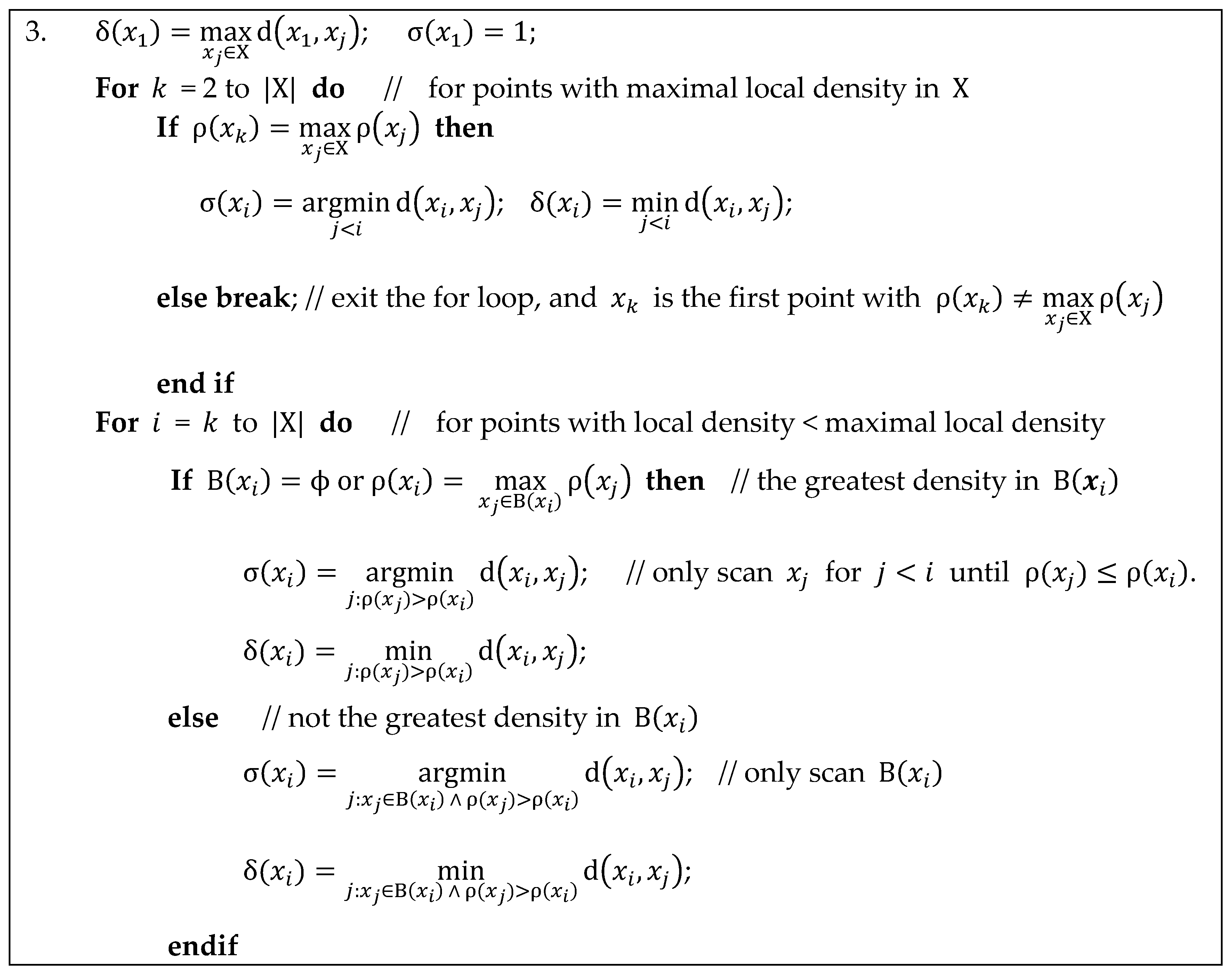
Appendix B. Implementation Details for Calculating Separation Distance in ADPC1

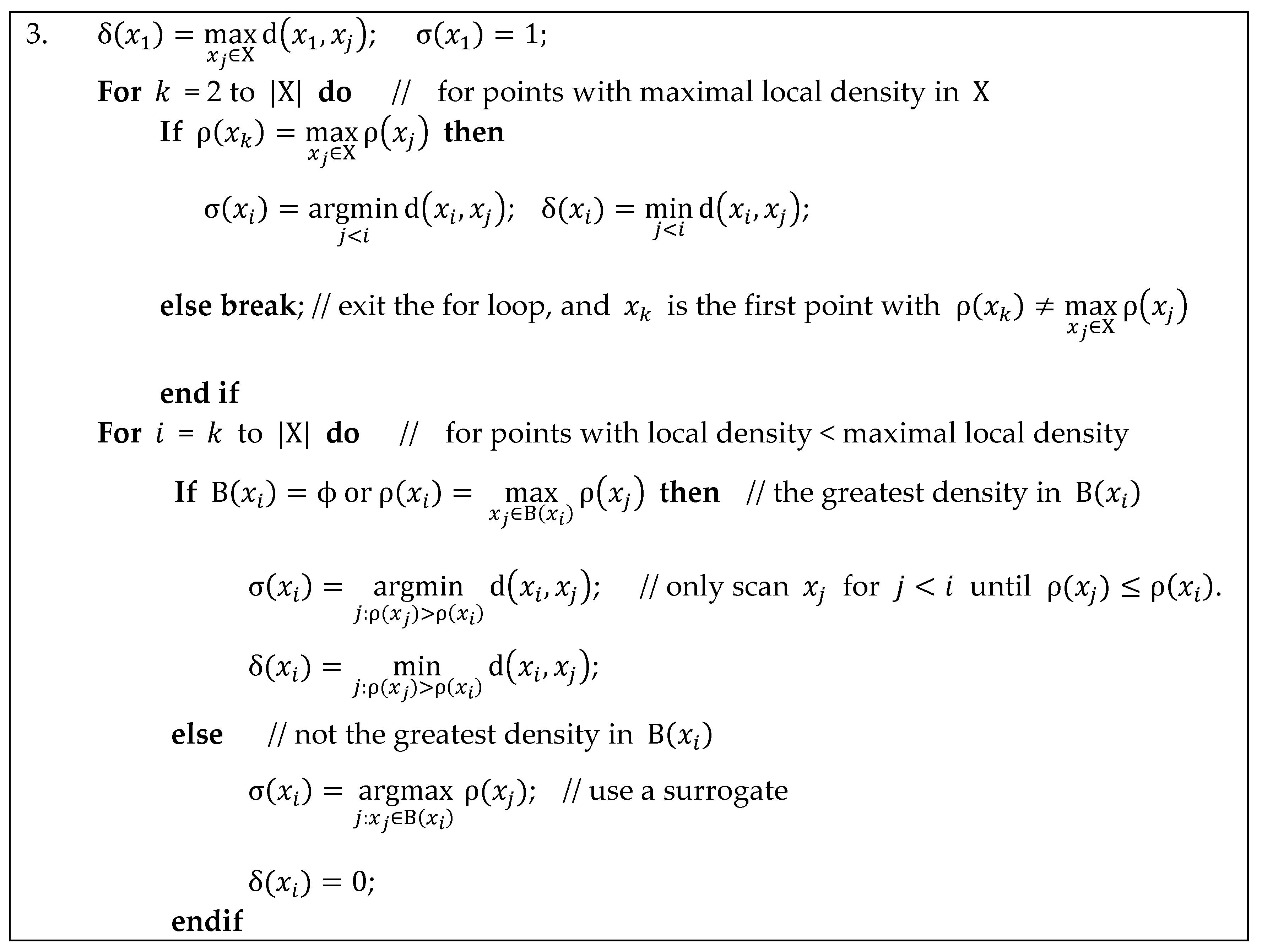
Appendix C. Implementation Details for Calculating Separation Distance in ADPC2

Appendix D. Datasets


| Dataset | Number of Clusters | Number of Points |
|---|---|---|
| Spiral | 3 | 312 |
| Flame | 2 | 240 |
| Aggregation | 7 | 788 |
| R15 | 15 | 600 |
| D31 | 31 | 3100 |
| A1 | 20 | 3000 |
| A2 | 35 | 5250 |
| A3 | 50 | 7500 |
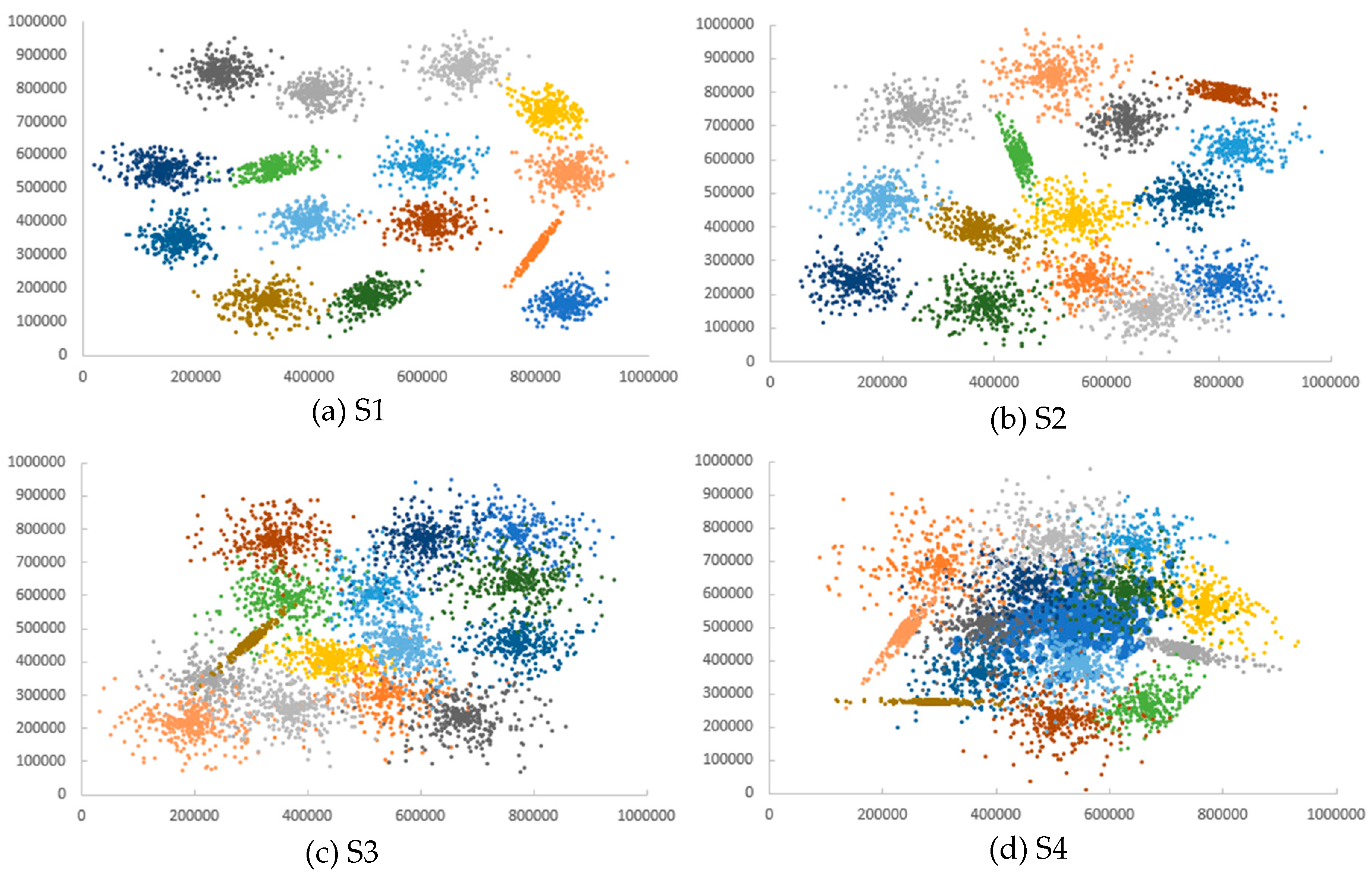
| S1 | 15 | 5000 |
| S2 | 15 | 5000 |
| S3 | 15 | 5000 |
| S4 | 15 | 5000 |
Appendix E. More Experimental Results
| Dataset (N) | p = 0.5 | p = 1 | p = 1.5 | p = 2 | p = 2.5 | p = 3 | p = 3.5 | p = 4 |
|---|---|---|---|---|---|---|---|---|
| Spiral (N = 312) | 62 | 90 | 110 | 139 | 161 | 187 | 208 | 232 |
| Flame (N = 240) | 75 | 143 | 177 | 208 | 213 | 221 | 226 | 231 |
| Aggregation (N = 788) | 609 | 704 | 744 | 760 | 763 | 761 | 761 | 768 |
| R15 (N = 600) | 348 | 490 | 537 | 558 | 563 | 570 | 564 | 567 |
| D31 (N = 3100) | 2952 | 3028 | 3034 | 3037 | 3013 | 2726 | 2034 | 2482 |
| A1 (N = 3000) | 2854 | 2955 | 2967 | 2968 | 2971 | 2973 | 2964 | 2962 |
| A2 (N = 5250) | 5140 | 5201 | 5192 | 5185 | 5202 | 5214 | 5236 | 5237 |
| A3 (N = 7500) | 7398 | 7418 | 7413 | 7456 | 7477 | 7483 | 7486 | 7490 |
| S1 (N = 5000) | 4305 | 4806 | 4912 | 4936 | 4945 | 4956 | 4974 | 4973 |
| S2 (N = 5000) | 4351 | 4834 | 4934 | 4953 | 4950 | 4954 | 4968 | 4961 |
| S3 (N = 5000) | 4474 | 4882 | 4942 | 4959 | 4977 | 4970 | 4977 | 4982 |
| S4 (N = 5000) | 4355 | 4818 | 4930 | 4955 | 4964 | 4968 | 4972 | 4976 |
| Dataset (N) | p = 0.5 | p = 1 | p = 1.5 | p = 2 | p = 2.5 | p = 3 | p = 3.5 | p = 4 |
|---|---|---|---|---|---|---|---|---|
| Spiral (N = 312) | 148 | 251 | 286 | 301 | 308 | 309 | 309 | 309 |
| Flame (N = 240) | 118 | 188 | 219 | 231 | 232 | 234 | 234 | 235 |
| Aggregation (N = 788) | 725 | 769 | 775 | 778 | 779 | 780 | 781 | 781 |
| R15 (N = 600) | 439 | 527 | 556 | 572 | 576 | 581 | 584 | 584 |
| D31 (N = 3100) | 2983 | 3044 | 3061 | 3067 | 3069 | 3070 | 3075 | 3085 |
| A1 (N = 3000) | 2914 | 2967 | 2977 | 2978 | 2980 | 2980 | 2981 | 2983 |
| A2 (N = 5250) | 5175 | 5212 | 5214 | 5216 | 5227 | 5236 | 5239 | 5243 |
| A3 (N = 7500) | 7424 | 7447 | 7453 | 7475 | 7483 | 7491 | 7493 | 7493 |
| S1 (N = 5000) | 4592 | 4880 | 4944 | 4963 | 4978 | 4983 | 4983 | 4984 |
| S2 (N = 5000) | 4605 | 4910 | 4968 | 4980 | 4982 | 4984 | 4985 | 4985 |
| S3 (N = 5000) | 4727 | 4932 | 4966 | 4979 | 4983 | 4985 | 4987 | 4988 |
| S4 (N = 5000) | 4652 | 4910 | 4953 | 4971 | 4974 | 4980 | 4985 | 4987 |
| Dataset | Algorithm | p = 0.5 | p = 1 | p = 1.5 | p = 2 | p = 2.5 | p = 3 | p = 3.5 | p = 4 |
|---|---|---|---|---|---|---|---|---|---|
| Spiral | DPC | 0.038101 | 0.046879 | 0.079211 | 0.052139 | 0.04688 | 0.046879 | 0.046879 | 0.046879 |
| ADPC1 | 0.035094 | 0.041108 | 0.036096 | 0.032086 | 0.046879 | 0.031252 | 0.031252 | 0.046879 | |
| ADPC2 | 0.04512 | 0.033088 | 0.04512 | 0.046878 | 0.031251 | 0.046845 | 0.04686 | 0.015646 | |
| Flame | DPC | 0.031253 | 0.031255 | 0.031273 | 0.031252 | 0.031253 | 0.031252 | 0.031252 | 0.031253 |
| ADPC1 | 0.015626 | 0.031253 | 0.015626 | 0 | 0.015599 | 0.015628 | 0 | 0.015628 | |
| ADPC2 | 0.031255 | 0.015625 | 0.015605 | 0.015627 | 0.015627 | 0 | 0.0156 | 0.015606 | |
| Aggregation | DPC | 0.252673 | 0.265685 | 0.281293 | 0.296938 | 0.296938 | 0.296938 | 0.312564 | 0.281312 |
| ADPC1 | 0.081215 | 0.078132 | 0.062506 | 0.062507 | 0.062506 | 0.078133 | 0.062506 | 0.078133 | |
| ADPC2 | 0.0781 | 0.062507 | 0.04688 | 0.04688 | 0.046901 | 0.062507 | 0.078133 | 0.062505 | |
| R15 | DPC | 0.156265 | 0.171892 | 0.171892 | 0.171892 | 0.171892 | 0.187519 | 0.171891 | 0.171891 |
| ADPC1 | 0.125012 | 0.078131 | 0.078131 | 0.04688 | 0.046879 | 0.04688 | 0.046873 | 0.046878 | |
| ADPC2 | 0.093759 | 0.07813 | 0.046879 | 0.046879 | 0.046878 | 0.031253 | 0.031253 | 0.031253 | |
| D31 | DPC | 4.281704 | 4.344213 | 4.375495 | 4.375465 | 4.375464 | 4.234823 | 3.187837 | 3.625386 |
| ADPC1 | 0.883543 | 0.7657 | 0.742746 | 0.781333 | 0.812588 | 0.937631 | 1.687681 | 1.672092 | |
| ADPC2 | 0.875124 | 0.71418 | 0.687573 | 0.7032 | 0.734489 | 0.828213 | 1.640798 | 1.578292 | |
| A1 | DPC | 4.016051 | 4.078557 | 4.125437 | 4.141065 | 4.145534 | 4.160485 | 4.234813 | 4.187945 |
| ADPC1 | 0.81259 | 0.687572 | 0.687606 | 0.734455 | 0.781332 | 0.79696 | 0.828212 | 0.89072 | |
| ADPC2 | 0.796961 | 0.656319 | 0.640726 | 0.67195 | 0.687573 | 0.687573 | 0.718826 | 0.762816 | |
| A2 | DPC | 12.48567 | 12.4857 | 12.59509 | 12.59508 | 12.59509 | 12.68885 | 12.76698 | 12.7982 |
| ADPC1 | 2.078376 | 1.984586 | 2.093839 | 2.203357 | 2.328372 | 2.484632 | 2.564224 | 2.672159 | |
| ADPC2 | 2.000502 | 1.922079 | 2.250205 | 2.000213 | 2.093969 | 2.187732 | 2.234609 | 2.297118 | |
| A3 | DPC | 25.42454 | 25.53396 | 25.69023 | 25.72854 | 26.01839 | 26.11215 | 26.40587 | 26.33089 |
| ADPC1 | 3.926412 | 4.189912 | 4.47909 | 4.547357 | 4.769292 | 5.194029 | 5.486006 | 5.506579 | |
| ADPC2 | 3.83774 | 3.802774 | 3.953544 | 4.1411 | 4.281703 | 4.420601 | 4.561412 | 4.742328 | |
| S1 | DPC | 11.42309 | 11.81372 | 11.65747 | 11.71463 | 11.75125 | 11.79816 | 11.79813 | 11.82938 |
| ADPC1 | 3.922292 | 2.422134 | 2.140852 | 2.125225 | 2.140851 | 2.234612 | 2.344002 | 2.437762 | |
| ADPC2 | 3.8584 | 2.328372 | 1.984588 | 1.93774 | 1.922111 | 1.953329 | 2.035082 | 2.125227 | |
| S2 | DPC | 11.21994 | 11.45434 | 11.52083 | 11.5481 | 11.68874 | 11.64186 | 11.65748 | 11.67311 |
| ADPC1 | 3.687891 | 2.312742 | 2.031496 | 2.062718 | 2.15648 | 2.218986 | 2.344 | 2.469012 | |
| ADPC2 | 3.641011 | 2.203357 | 1.906452 | 1.890826 | 1.922079 | 1.984584 | 2.047092 | 2.105681 | |
| S3 | DPC | 11.29808 | 11.48559 | 11.56373 | 11.56373 | 11.62623 | 11.59498 | 11.65748 | 11.67311 |
| ADPC1 | 3.21909 | 2.14085 | 2.031468 | 2.031467 | 2.109567 | 2.234612 | 2.343999 | 2.469044 | |
| ADPC2 | 3.187838 | 2.015836 | 1.890857 | 1.86247 | 1.906452 | 1.97208 | 2.031466 | 2.109599 | |
| S4 | DPC | 11.25118 | 11.51685 | 11.57936 | 11.62623 | 11.56371 | 11.64183 | 11.71999 | 11.70437 |
| ADPC1 | 3.515999 | 2.344002 | 2.078346 | 2.093971 | 2.203359 | 2.265865 | 2.359625 | 2.437758 | |
| ADPC2 | 3.484713 | 2.250242 | 1.937706 | 1.906451 | 1.968992 | 1.984586 | 2.062751 | 2.099317 |
| Dataset | Algorithm | p = 0.5 | p = 1 | p = 1.5 | p = 2 | p = 2.5 | p = 3 | p = 3.5 | p = 4 |
|---|---|---|---|---|---|---|---|---|---|
| Spiral | DPC | 0.217607 | 0.227606 | 0.24064 | 0.230642 | 0.218788 | 0.234399 | 0.218773 | 0.218806 |
| ADPC1 | 0.243648 | 0.210588 | 0.199559 | 0.177449 | 0.17189 | 0.218742 | 0.171892 | 0.187521 | |
| ADPC2 | 0.201514 | 0.179477 | 0.177471 | 0.215608 | 0.171891 | 0.18752 | 0.171869 | 0.171893 | |
| Flame | DPC | 0.12501 | 0.125012 | 0.125014 | 0.14064 | 0.125013 | 0.14064 | 0.125014 | 0.14064 |
| ADPC1 | 0.109386 | 0.109386 | 0.109386 | 0.125014 | 0.093759 | 0.109406 | 0.109387 | 0.109387 | |
| ADPC2 | 0.12501 | 0.109385 | 0.125013 | 0.109386 | 0.10938 | 0.109386 | 0.109384 | 0.109385 | |
| Aggregation | DPC | 1.299488 | 1.250166 | 1.250131 | 1.281362 | 1.281407 | 1.250169 | 1.250164 | 1.250162 |
| ADPC1 | 1.078868 | 1.062644 | 1.062612 | 1.062614 | 1.062644 | 1.062645 | 1.078269 | 1.078274 | |
| ADPC2 | 1.11083 | 1.062613 | 1.046983 | 1.047022 | 1.047018 | 1.047019 | 1.047018 | 1.047018 | |
| R15 | DPC | 0.779632 | 0.750111 | 0.750057 | 0.750113 | 0.750075 | 0.765738 | 0.734483 | 0.73445 |
| ADPC1 | 0.703232 | 0.671957 | 0.656351 | 0.640727 | 0.656351 | 0.640728 | 0.625097 | 0.625066 | |
| ADPC2 | 0.703232 | 0.671978 | 0.656351 | 0.625098 | 0.640724 | 0.640691 | 0.625097 | 0.60947 | |
| D31 | DPC | 20.34588 | 19.8146 | 19.90442 | 19.53329 | 19.65834 | 19.5177 | 19.54898 | 19.64271 |
| ADPC1 | 17.12682 | 16.74525 | 16.61117 | 16.39237 | 16.56423 | 16.39233 | 16.4581 | 16.59551 | |
| ADPC2 | 17.11119 | 16.64242 | 16.36111 | 16.25173 | 16.28676 | 16.35301 | 16.53297 | 16.37674 | |
| A1 | DPC | 18.58013 | 18.08004 | 17.95503 | 17.98625 | 17.8769 | 17.8988 | 17.95503 | 17.8769 |
| ADPC1 | 15.57978 | 15.26725 | 15.18911 | 15.15783 | 15.12657 | 15.15679 | 15.16565 | 15.19659 | |
| ADPC2 | 15.42351 | 15.15789 | 15.04847 | 15.01722 | 14.90703 | 15.00159 | 14.92343 | 14.87658 | |
| A2 | DPC | 56.31846 | 55.53715 | 55.05268 | 55.67778 | 55.25958 | 55.44339 | 55.5684 | 55.64653 |
| ADPC1 | 47.64571 | 46.62474 | 46.12989 | 46.31741 | 47.2863 | 46.45805 | 46.27054 | 46.87997 | |
| ADPC2 | 47.3644 | 46.12753 | 45.97363 | 46.37992 | 46.12989 | 45.84858 | 45.91012 | 46.16624 | |
| A3 | DPC | 115.6921 | 112.1025 | 112.9651 | 115.0125 | 112.3618 | 112.9651 | 112.1213 | 112.8714 |
| ADPC1 | 95.73069 | 93.50614 | 95.91672 | 95.73115 | 95.51016 | 94.68273 | 95.79348 | 96.21016 | |
| ADPC2 | 96.21336 | 94.86226 | 94.79854 | 93.96594 | 94.73864 | 93.69754 | 94.52285 | 94.63775 | |
| S1 | DPC | 53.11501 | 51.63048 | 50.92332 | 50.58346 | 50.44285 | 50.78661 | 50.19283 | 51.5836 |
| ADPC1 | 45.36419 | 43.80152 | 42.70859 | 42.8327 | 42.33265 | 42.0513 | 42.2279 | 42.50451 | |
| ADPC2 | 45.77048 | 43.614 | 42.9889 | 41.89504 | 42.33735 | 41.86379 | 41.8169 | 41.92629 | |
| S2 | DPC | 51.88047 | 50.97416 | 50.89606 | 50.00531 | 50.36472 | 50.08341 | 50.73976 | 50.56783 |
| ADPC1 | 44.75324 | 42.71937 | 42.00446 | 42.00442 | 42.22323 | 44.39533 | 42.66078 | 42.61389 | |
| ADPC2 | 44.58285 | 42.48891 | 41.85598 | 41.86382 | 41.86418 | 41.7544 | 41.9107 | 41.75443 | |
| S3 | DPC | 51.89613 | 50.14595 | 50.17026 | 49.89592 | 50.03655 | 50.63037 | 50.13029 | 50.03656 |
| ADPC1 | 43.45777 | 41.86382 | 41.75443 | 41.78568 | 41.64504 | 41.86382 | 42.22323 | 41.88364 | |
| ADPC2 | 44.23907 | 41.84819 | 42.20761 | 41.77006 | 42.27011 | 41.65029 | 41.87944 | 41.89504 | |
| S4 | DPC | 51.45296 | 50.1772 | 50.42723 | 50.5679 | 50.36469 | 50.05215 | 50.00527 | 50.23967 |
| ADPC1 | 44.00467 | 42.13493 | 41.84819 | 42.52013 | 42.05134 | 42.00442 | 42.274 | 42.28573 | |
| ADPC2 | 44.47347 | 41.88291 | 42.08256 | 42.03568 | 42.17635 | 41.66067 | 41.86382 | 41.84976 |
References
- Aggarwal, C.C.; Reddy, C.K. Data Clustering: Algorithms and Applications; Chapman and Hall/CRC: Boca Raton, FL, USA, 2014. [Google Scholar]
- Pham, G.; Lee, S.-H.; Kwon, O.-H.; Kwon, K.-R. A watermarking method for 3d printing based on menger curvature and k-mean clustering. Symmetry 2018, 10, 97. [Google Scholar] [CrossRef]
- MacQueen, J. Some methods for classification and analysis of multivariate observations. In Proceedings of the Fifth Berkeley Symposium on Mathematical Statistics and Probability, Berkeley, CA, USA, 18–21 June 1965; pp. 281–297. [Google Scholar]
- Ester, M.; Kriegel, H.-P.; Sander, J.; Xu, X. A density-based algorithm for discovering clusters a density-based algorithm for discovering clusters in large spatial databases with noise. KDD 1996, 96, 226–231. [Google Scholar]
- Han, J.; Kamber, M.; Pei, J. Data Mining: Concepts and Techniques; Morgan Kaufmann Publishers Inc.: San Francisco, CA, USA, 2011; p. 696. [Google Scholar]
- Rodriguez, A.; Laio, A. Clustering by fast search and find of density peaks. Science 2014, 344, 1492. [Google Scholar] [CrossRef] [PubMed]
- Mehmood, R.; Zhang, G.; Bie, R.; Dawood, H.; Ahmad, H. Clustering by fast search and find of density peaks via heat diffusion. Neurocomputing 2016, 208, 210–217. [Google Scholar] [CrossRef]
- Wang, S.; Wang, D.; Li, C.; Li, Y.; Ding, G. Clustering by fast search and find of density peaks with data field. Chin. J. Electron. 2016, 25, 397–402. [Google Scholar] [CrossRef]
- Bai, L.; Cheng, X.; Liang, J.; Shen, H.; Guo, Y. Fast density clustering strategies based on the k-means algorithm. Pattern Recognit. 2017, 71, 375–386. [Google Scholar] [CrossRef]
- Mehmood, R.; El-Ashram, S.; Bie, R.; Dawood, H.; Kos, A. Clustering by fast search and merge of local density peaks for gene expression microarray data. Sci. Rep. 2017, 7, 45602. [Google Scholar] [CrossRef]
- Liu, S.; Zhou, B.; Huang, D.; Shen, L. Clustering mixed data by fast search and find of density peaks. Math. Probl. Eng. 2017, 2017, 7. [Google Scholar] [CrossRef]
- Li, Z.; Tang, Y. Comparative density peaks clustering. Expert Syst. Appl. 2018, 95, 236–247. [Google Scholar] [CrossRef]
- Du, M.; Ding, S.; Jia, H. Study on density peaks clustering based on k-nearest neighbors and principal component analysis. Knowl.-Based Syst. 2016, 99, 135–145. [Google Scholar] [CrossRef]
- Yaohui, L.; Zhengming, M.; Fang, Y. Adaptive density peak clustering based on k-nearest neighbors with aggregating strategy. Knowl.-Based Syst. 2017, 133, 208–220. [Google Scholar] [CrossRef]
- Ding, S.; Du, M.; Sun, T.; Xu, X.; Xue, Y. An entropy-based density peaks clustering algorithm for mixed type data employing fuzzy neighborhood. Knowl.-Based Syst. 2017, 133, 294–313. [Google Scholar] [CrossRef]
- Yang, X.-H.; Zhu, Q.-P.; Huang, Y.-J.; Xiao, J.; Wang, L.; Tong, F.-C. Parameter-free laplacian centrality peaks clustering. Pattern Recognit. Lett. 2017, 100, 167–173. [Google Scholar] [CrossRef]
- Cheng, S.; Duan, Y.; Fan, X.; Zhang, D.; Cheng, H. Review of Fast Density-Peaks Clustering and Its Application to Pediatric White Matter Tracts. In Annual Conference on Medical Image Understanding and Analysis; Springer International Publishing: Cham, Switzerland, 2017; pp. 436–447. [Google Scholar]
- Han, J.; Kamber, M.; Pei, J. 10-cluster analysis: Basic concepts and methods. In Data Mining, 3rd ed.; Han, J., Kamber, M., Pei, J., Eds.; Morgan Kaufmann: Boston, MA, USA, 2012; pp. 443–495. [Google Scholar]
- Xenaki, S.D.; Koutroumbas, K.D.; Rontogiannis, A.A. A novel adaptive possibilistic clustering algorithm. IEEE Trans. Fuzzy Syst. 2016, 24, 791–810. [Google Scholar] [CrossRef]
- Bianchi, G.; Bruni, R.; Reale, A.; Sforzi, F. A min-cut approach to functional regionalization, with a case study of the italian local labour market areas. Optim. Lett. 2016, 10, 955–973. [Google Scholar] [CrossRef]
- Deng, Z.; Choi, K.-S.; Jiang, Y.; Wang, J.; Wang, S. A survey on soft subspace clustering. Inf. Sci. 2016, 348, 84–106. [Google Scholar] [CrossRef]
- Laio, A. Matlab Implementation of the Density Peak Algorithm. Available online: http://people.sissa.it/~laio/Research/Clustering_source_code/cluster_dp.tgz (accessed on 27 May 2019).
- Chang, H.; Yeung, D.-Y. Robust path-based spectral clustering. Pattern Recognit. 2008, 41, 191–203. [Google Scholar] [CrossRef]
- Fu, L.; Medico, E. Flame, a novel fuzzy clustering method for the analysis of DNA microarray data. BMC Bioinf. 2007, 8, 3. [Google Scholar] [CrossRef]
- Gionis, A.; Mannila, H.; Tsaparas, P. Clustering aggregation. ACM Trans. Knowl. Discov. Data 2007, 1, 4. [Google Scholar] [CrossRef]
- Veenman, C.J.; Reinders, M.J.T.; Backer, E. A maximum variance cluster algorithm. IEEE Trans. Pattern Anal. Mach. Intell. 2002, 24, 1273–1280. [Google Scholar] [CrossRef]
- Kärkkäinen, I.; Fränti, P. Dynamic Local Search Algorithm for the Clustering Problem; University of Joensuu: Joensuu, Finland, 2002. [Google Scholar]
- Fränti, P.; Virmajoki, O. Iterative shrinking method for clustering problems. Pattern Recognit. 2006, 39, 761–775. [Google Scholar] [CrossRef]
- Lin, J.; Peng, H.; Xie, J.; Zheng, Q. Novel clustering algorithm based on central symmetry. In Proceedings of the Internation Conference on Machine Learning and Cybernetics, Shanghai, China, 26–29 August 2004; pp. 1329–1334. [Google Scholar]
- Bandyopadhyay, S.; Saha, S. A Point Symmetry-Based Clustering Technique for Automatic Evolution of Clusters. IEEE Trans. Knowl. Data Eng. 2008, 20, 1441–1457. [Google Scholar] [CrossRef]
| Dataset | p = 0.5 | p = 1 | p = 1.5 | p = 2 | p = 2.5 | p = 3 | p = 3.5 | p = 4 |
|---|---|---|---|---|---|---|---|---|
| Spiral | 19.87% | 28.85% | 35.26% | 44.55% | 51.60% | 59.94% | 66.67% | 74.36% |
| Flame | 31.25% | 59.58% | 73.75% | 86.67% | 88.75% | 92.08% | 94.17% | 96.25% |
| Aggregation | 77.28% | 89.34% | 94.42% | 96.45% | 96.83% | 96.57% | 96.57% | 97.46% |
| R15 | 58.00% | 81.67% | 89.50% | 93.00% | 93.83% | 95.00% | 94.00% | 94.50% |
| D31 | 95.23% | 97.68% | 97.87% | 97.97% | 97.19% | 87.94% | 65.61% | 80.06% |
| A1 | 95.13% | 98.50% | 98.90% | 98.93% | 99.03% | 99.10% | 98.80% | 98.73% |
| A2 | 97.90% | 99.07% | 98.90% | 98.76% | 99.09% | 99.31% | 99.73% | 99.75% |
| A3 | 98.64% | 98.91% | 98.84% | 99.41% | 99.69% | 99.77% | 99.81% | 99.87% |
| S1 | 86.10% | 96.12% | 98.24% | 98.72% | 98.90% | 99.12% | 99.48% | 99.46% |
| S2 | 87.02% | 96.68% | 98.68% | 99.06% | 99.00% | 99.08% | 99.36% | 99.22% |
| S3 | 89.48% | 97.64% | 98.84% | 99.18% | 99.54% | 99.40% | 99.54% | 99.64% |
| S4 | 87.10% | 96.36% | 98.60% | 99.10% | 99.28% | 99.36% | 99.44% | 99.52% |
| Dataset | Algorithm | p = 0.5 | p = 1 | p = 1.5 | p = 2 | p = 2.5 | p = 3 | p = 3.5 | p = 4 |
|---|---|---|---|---|---|---|---|---|---|
| Spiral | ADPC1 | 7.89% | 12.31% | 54.43% | 38.46% | 0.00% | 33.33% | 33.33% | 0.00% |
| ADPC2 | –18.42% | 29.42% | 43.04% | 10.09% | 33.34% | 0.07% | 0.04% | 66.62% | |
| Flame | ADPC1 | 50.00% | 0.01% | 50.03% | 100.00% | 50.09% | 49.99% | 100.00% | 50.00% |
| ADPC2 | −0.01% | 50.01% | 50.10% | 50.00% | 50.00% | 100.00% | 50.08% | 50.07% | |
| Aggregation | ADPC1 | 67.86% | 70.59% | 77.78% | 78.95% | 78.95% | 73.69% | 80.00% | 72.23% |
| ADPC2 | 69.09% | 76.47% | 83.33% | 84.21% | 84.21% | 78.95% | 75.00% | 77.78% | |
| R15 | ADPC1 | 20.00% | 54.55% | 54.55% | 72.73% | 72.73% | 75.00% | 72.73% | 72.73% |
| ADPC2 | 40.00% | 54.55% | 72.73% | 72.73% | 72.73% | 83.33% | 81.82% | 81.82% | |
| D31 | ADPC1 | 79.36% | 82.37% | 83.02% | 82.14% | 81.43% | 77.86% | 47.06% | 53.88% |
| ADPC2 | 79.56% | 83.56% | 84.29% | 83.93% | 83.21% | 80.44% | 48.53% | 56.47% | |
| A1 | ADPC1 | 79.77% | 83.14% | 83.33% | 82.26% | 81.15% | 80.84% | 80.44% | 78.73% |
| ADPC2 | 80.16% | 83.91% | 84.47% | 83.77% | 83.41% | 83.47% | 83.03% | 81.79% | |
| A2 | ADPC1 | 83.35% | 84.11% | 83.38% | 82.51% | 81.51% | 80.42% | 79.92% | 79.12% |
| ADPC2 | 83.98% | 84.61% | 82.13% | 84.12% | 83.37% | 82.76% | 82.50% | 82.05% | |
| A3 | ADPC1 | 84.56% | 83.59% | 82.57% | 82.33% | 81.67% | 80.11% | 79.22% | 79.09% |
| ADPC2 | 84.91% | 85.11% | 84.61% | 83.90% | 83.54% | 83.07% | 82.73% | 81.99% | |
| S1 | ADPC1 | 65.66% | 79.50% | 81.64% | 81.86% | 81.78% | 81.06% | 80.13% | 79.39% |
| ADPC2 | 66.22% | 80.29% | 82.98% | 83.46% | 83.64% | 83.44% | 82.75% | 82.03% | |
| S2 | ADPC1 | 67.13% | 79.81% | 82.37% | 82.14% | 81.55% | 80.94% | 79.89% | 78.85% |
| ADPC2 | 67.55% | 80.76% | 83.45% | 83.63% | 83.56% | 82.95% | 82.44% | 81.96% | |
| S3 | ADPC1 | 71.51% | 81.36% | 82.43% | 82.43% | 81.86% | 80.73% | 79.89% | 78.85% |
| ADPC2 | 71.78% | 82.45% | 83.65% | 83.89% | 83.60% | 82.99% | 82.57% | 81.93% | |
| S4 | ADPC1 | 68.75% | 79.65% | 82.05% | 81.99% | 80.95% | 80.54% | 79.87% | 79.17% |
| ADPC2 | 69.03% | 80.46% | 83.27% | 83.60% | 82.97% | 82.95% | 82.40% | 82.06% |
| Dataset | p = 0.5 | p = 1 | p = 1.5 | p = 2 | p = 2.5 | p = 3 | p = 3.5 | p = 4 |
|---|---|---|---|---|---|---|---|---|
| Spiral | 47.44% | 80.45% | 91.67% | 96.47% | 98.72% | 99.04% | 99.04% | 99.04% |
| Flame | 49.17% | 78.33% | 91.25% | 96.25% | 96.67% | 97.50% | 97.50% | 97.92% |
| Aggregation | 92.01% | 97.59% | 98.35% | 98.73% | 98.86% | 98.98% | 99.11% | 99.11% |
| R15 | 73.17% | 87.83% | 92.67% | 95.33% | 96.00% | 96.83% | 97.33% | 97.33% |
| D31 | 96.23% | 98.19% | 98.74% | 98.94% | 99.00% | 99.03% | 99.19% | 99.52% |
| A1 | 97.13% | 98.90% | 99.23% | 99.27% | 99.33% | 99.33% | 99.37% | 99.43% |
| A2 | 98.57% | 99.28% | 99.31% | 99.35% | 99.56% | 99.73% | 99.79% | 99.87% |
| A3 | 98.99% | 99.29% | 99.37% | 99.67% | 99.77% | 99.88% | 99.91% | 99.91% |
| S1 | 91.84% | 97.60% | 98.88% | 99.26% | 99.56% | 99.66% | 99.66% | 99.68% |
| S2 | 92.10% | 98.20% | 99.36% | 99.60% | 99.64% | 99.68% | 99.70% | 99.70% |
| S3 | 94.54% | 98.64% | 99.32% | 99.58% | 99.66% | 99.70% | 99.74% | 99.76% |
| S4 | 93.04% | 98.20% | 99.06% | 99.42% | 99.48% | 99.60% | 99.70% | 99.74% |
| Dataset | Algorithm | p = 0.5 | p = 1 | p = 1.5 | p = 2 | p = 2.5 | p = 3 | p = 3.5 | p = 4 |
|---|---|---|---|---|---|---|---|---|---|
| Spiral | ADPC1 | –11.97% | 7.48% | 17.07% | 23.06% | 21.44% | 6.68% | 21.43% | 14.30% |
| ADPC2 | 7.40% | 21.15% | 26.25% | 6.52% | 21.43% | 20.00% | 21.44% | 21.44% | |
| Flame | ADPC1 | 12.50% | 12.50% | 12.50% | 11.11% | 25.00% | 22.21% | 12.50% | 22.22% |
| ADPC2 | 0.00% | 12.50% | 0.001% | 22.22% | 12.51% | 22.22% | 12.50% | 22.22% | |
| Aggregation | ADPC1 | 16.98% | 15.00% | 15.00% | 17.07% | 17.07% | 15.00% | 13.75% | 13.75% |
| ADPC2 | 14.52% | 15.00% | 16.25% | 18.29% | 18.29% | 16.25% | 16.25% | 16.25% | |
| R15 | ADPC1 | 9.80% | 10.42% | 12.49% | 14.58% | 12.50% | 16.33% | 14.89% | 14.89% |
| ADPC2 | 9.80% | 10.42% | 12.49% | 16.67% | 14.58% | 16.33% | 14.89% | 17.02% | |
| D31 | ADPC1 | 15.82% | 15.49% | 16.55% | 16.08% | 15.74% | 16.01% | 15.81% | 15.51% |
| ADPC2 | 15.90% | 16.01% | 17.80% | 16.80% | 17.15% | 16.21% | 15.43% | 16.63% | |
| A1 | ADPC1 | 16.15% | 15.56% | 15.40% | 15.73% | 15.38% | 15.32% | 15.54% | 14.99% |
| ADPC2 | 16.99% | 16.16% | 16.19% | 16.51% | 16.61% | 16.19% | 16.88% | 16.78% | |
| A2 | ADPC1 | 15.40% | 16.05% | 16.21% | 16.81% | 14.43% | 16.21% | 16.73% | 15.75% |
| ADPC2 | 15.90% | 16.94% | 16.49% | 16.70% | 16.52% | 17.31% | 17.38% | 17.04% | |
| A3 | ADPC1 | 17.25% | 16.59% | 15.09% | 16.76% | 15.00% | 16.18% | 14.56% | 14.76% |
| ADPC2 | 16.84% | 15.38% | 16.08% | 18.30% | 15.68% | 17.06% | 15.70% | 16.15% | |
| S1 | ADPC1 | 14.59% | 15.16% | 16.13% | 15.32% | 16.08% | 17.20% | 15.87% | 17.60% |
| ADPC2 | 13.83% | 15.53% | 15.58% | 17.18% | 16.07% | 17.57% | 16.69% | 18.72% | |
| S2 | ADPC1 | 13.74% | 16.19% | 17.47% | 16.00% | 16.17% | 11.36% | 15.92% | 15.73% |
| ADPC2 | 14.07% | 16.65% | 17.76% | 16.28% | 16.88% | 16.63% | 17.40% | 17.43% | |
| S3 | ADPC1 | 16.26% | 16.52% | 16.77% | 16.25% | 16.77% | 17.31% | 15.77% | 16.29% |
| ADPC2 | 14.75% | 16.55% | 15.87% | 16.29% | 15.52% | 17.74% | 16.46% | 16.27% | |
| S4 | ADPC1 | 14.48% | 16.03% | 17.01% | 15.91% | 16.51% | 16.08% | 15.46% | 15.83% |
| ADPC2 | 13.56% | 16.53% | 16.55% | 16.87% | 16.26% | 16.77% | 16.28% | 16.70% |
© 2019 by the author. Licensee MDPI, Basel, Switzerland. This article is an open access article distributed under the terms and conditions of the Creative Commons Attribution (CC BY) license (http://creativecommons.org/licenses/by/4.0/).
Share and Cite
Lin, J.-L. Accelerating Density Peak Clustering Algorithm. Symmetry 2019, 11, 859. https://doi.org/10.3390/sym11070859
Lin J-L. Accelerating Density Peak Clustering Algorithm. Symmetry. 2019; 11(7):859. https://doi.org/10.3390/sym11070859
Chicago/Turabian StyleLin, Jun-Lin. 2019. "Accelerating Density Peak Clustering Algorithm" Symmetry 11, no. 7: 859. https://doi.org/10.3390/sym11070859
APA StyleLin, J.-L. (2019). Accelerating Density Peak Clustering Algorithm. Symmetry, 11(7), 859. https://doi.org/10.3390/sym11070859