3D Flow Entropy Contour Fitting Segmentation Algorithm Based on Multi-Scale Transform Contour Constraint

Abstract

Image segmentation is a crucial topic in image analysis and understanding, and the foundation of target detection and recognition. Image segmentation, essentially, can be considered as classifying the image according to the consistency of the region and the inconsistency between regions, it is widely used in medical and criminal investigation, cultural relic identification, monitoring and so forth. There are two outstanding common problems in the existing segmentation algorithm, one is the lack of accuracy, and the other is that it is not widely applicable. The main contribution of this paper is to present a novel segmentation method based on the information entropy theory and multi-scale transform contour constraint. Firstly, the target contour is initially obtained by means of a multi-scale sample top-hat and bottom-hat transform and an improved watershed method. Subsequently, in terms of this initial contour, the interesting areas can be finely segmented out with an innovative 3D flow entropy method. Finally, the sufficient synthetic and real experiments proved that the proposed algorithm can greatly improve the segmentation effect. In addition, it is widely applicable.

1. Introduction

Image segmentation is an important technology of image analysis, and its results often determine the effect of image recognition. It has been widely used in medical and criminal investigation, cultural relic identification, monitoring and other areas. The main task of image segmentation is to obtain a region of interest from the image. Due to the significance of image segmentation, numerous researchers focus great attention on it.

Classic segmentation methods include the Otsu method, maximum entropy method [1,2], watershed algorithm [3], active contour method [4,5,6] and so on. Among them, the Otsu method uses selection of the global optimal threshold to segment an image. This method shows an ideal segmentation effect when the image histogram has the form of a double-peak. However, it is vulnerable to noise and image contrast. The maximum entropy method is a kind of statistic-based method that employs maximum information entropy to extract a target edge, and because of the pixel confusion in the noisy concentrated region, this method is likely to mistakenly identify the noise area as the target profile, which leads to the worse accuracy than Otsu. The watershed algorithm is a morphological segmentation algorithm, it tends to produce an over segmentation phenomenon if an image contains multiple target segmentation results. The active contour method uses the energy theory. The algorithm achieves great results when targets have a relatively convex contour line. However, this algorithm cannot satisfactorily deal with a target that has a concave contour. In view of the defects of the classical segmentation algorithms, researchers have made a lot of improvements to the existing classical segmentation algorithms in recent years. They can be approximately divided into three different directions: threshold methods, clustering methods and conditional constraint methods. In threshold methods, Li et al. [7] proposed an improved two-dimensional histogram partitioning threshold segmentation method, which uses two straight lines by threshold vector point and gray level shafts, respectively into the $\alpha$ and $\beta$ angle to partition a two-dimensional histogram. In this way, the threshold segmentation can be used on a wider range of applications, but for low contrast images, the segmentation effect of this method is not ideal. Fan et al. [8] further proposed a three-dimensional Otsu segmentation method which extended the two-dimensional histogram to the three-dimensional. This method greatly optimized the classical Otsu method, and the image with low contrast and low signal to noise ratio has a better segmentation effect. However, the threshold is still a global threshold, and the detail of the segmentation is not clear. Coupled with the complexity of the computation, the overall effect of the segmentation needs to be improved. Gao et al. [9] proposed a new watershed image segmentation algorithm based on markers, which directly used the watershed to segment the original gradient image. Hongnan Liang et al. [10] adopted a modified grasshopper optimization algorithm (GOA) to render multilevel Tsallis cross entropy more practical and reduce the complexity. Satish Rapaka et al. [11] proposed an efficient method for the segmentation of iris images that deal with non-circular iris boundaries. C. Zhang et al. [12] proposed a real-time segmentation method that separates the target signal from the navigation image. Qingyong Li et al. [13] proposed a double-scale non-linear thresholding method based on vessel support regions. In clustering methods, Zheng et al. [14] proposed the improved gray image maximum entropy segmentation method to replace the gray probability by the spatial information value and the two-dimensional difference attribute information entropy is generated. The algorithm has anti-noise ability. However, because of the lack of statistical information, when the image target is densely stacked, the segmentation result is not ideal. Wu et al. [15] proposed a contour of body of tongue image segmentation algorithm based on watershed transform and an active contour model, which used the result of the watershed transform as the initial curve of the active contour model algorithm. The segmentation effect can be improved to a certain extent, but the contour line in the target depression could not provide a normal component of force, and the segmentation effect for the target that has a depressed part is not ideal. Arbelaez’s [16] segmentation algorithm consists of generic machinery for transforming the output of any contour detector into a hierarchical region tree. L. Li, et al. [17] introduced background prior and object-center prior into infrared pedestrian segmentation and proposed a robust and efficient saliency-based scheme. In conditional constraint methods, Chen [18] proposed a new method that integrates the newly developed constrained spectral variance difference (CSVD) and the edge penalty (EP). Montoya et al. [19] discussed and evaluated parallel implementations of a segmentation algorithm based on the split-and-merge approach to solve the region growing problem. Haris et al. [20] proposed a hybrid multidimensional image segmentation algorithm. Soille [21] introduced an image partitioning and simplification method based on the constrained connectivity paradigm. Boyuan Ma et al. [22] trained a deep convolutional neural network based on DeepLab to achieve image segmentation and have significant results. Vijay Badrinarayanan et al. [23] present a novel and practical deep fully convolutional neural network architecture for semantic pixel-wise segmentation termed SegNet. Shervin Minaee et al. [24] proposed an algorithm for separating the foreground (mainly text and line graphics) from the smoothly varying background in screen content images. Liang-Chieh Chen et al. [25] proposed an attention mechanism that learns to softly weight the multi-scale features at each pixel location. Annegreet Van Opbroek et al. [26] proposed a new image weighting segmentation method that minimizes maximum mean discrepancy (MMD) between training and test data. Chen et al. [27] designed modules which employ atrous convolution in cascade or in parallel to capture multi-scale context by adopting multiple atrous rates. Shervin Minaee et al. [28] found a binary mask which shows the location of each image-component to make a synthesis of the above-mentioned segmentation method. Although having the effect of innovation in their respective fields, they still cannot solve the common problems of the existing algorithms.

This paper puts forward an algorithm innovation aiming at the two outstanding hot spots of the current research work—the effect of segmentation and the scope of application of the algorithm. First, a method for determining the initial contour line is proposed. The method uses top-hat and bottom-hat transform with multi-scale structure and the morphological segmentation method by adding the weighted vector cosine distance check to the select threshold in the initial region of interest. Experiments show that the algorithm greatly improves the running efficiency and reduces the over segmentation phenomenon. Second, the method proposes the establishment of a new three-dimensional coordinate system using the mean of skewness, median of skewness and gradient. Based on the information entropy and energy theory, the concept of flow entropy is proposed to segment the initial contour finely. The experimental results show that the proposed algorithm can solve the ubiquitous problem in the current information entropy edge detection and energy edge detection, which is inaccurate segmentation of the depressed area, low contrast region and noise region.

This paper is organized as follows. The first section introduces the significance of the topic, analysis of international research status and innovation points. The second section introduces the method of determining the initial contour line. In Section 2.1, the target image is pre-processed by the improved top-hat and bottom-hat transform. In Section 2.2, the high dimensional watershed algorithm is used to segment, and the weighted the vector cosine distance is finally added to ensure that the over segmentation phenomenon of the initial segmentation is reduced, as well as the more accurate region of interest. In the third section, the paper introduces the fine segmentation of the contour line. In Section 3.1, a new 3D segmentation model is established. In Section 3.2, the initial contour is finely segmented by the information entropy and energy restriction. The fourth section is the experimental results. This paper, in order to prove the segmentation effect and field of application, makes a comparison with existing image segmentation algorithms through three different types of image data as the experimental material. The fifth section summarizes the full text.

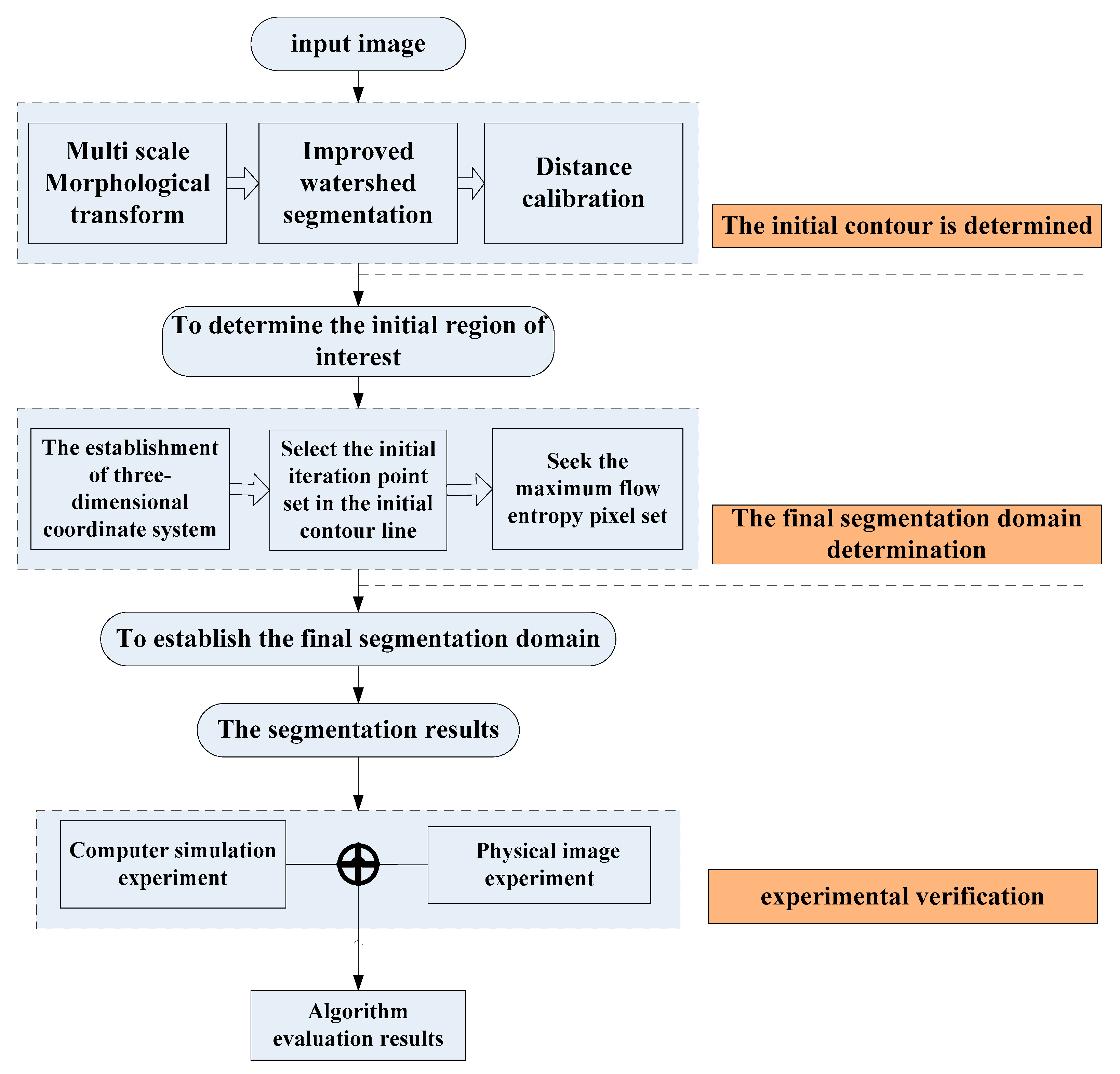
2. The Determination of the Initial Contour by Multi-Scale Morphological Fitting

Firstly, initial segmentation is carried out, by which the general region of interest for the image is selected. The initial segmentation can improve the accuracy of the segmentation.

2.1. Improved Top-Hat and Bottom-Hat Transform Sample Pretreatment

The top-hat and bottom-hat transform is an ideal technology for processing an image in primary vision [29,30,31]. Firstly, it can balance the brightness of the image and extract the inapparent target in the low contrast regions. Secondly, it can suppress the point source noise in the background. Top-hat transformation of a gray image $f$ is defined as $f$ subtracting its opening operation. Similarly, bottom-hat transformation of a gray image $f$ is defined as closing operation of minus $f$. This algorithm removes objects from an image by an opening or closing operation, instead of fitting the deleted object. Then, the image without the deleted component is obtained by the difference operation. The top-hat transformation is used for the bright objects in the dark background, while the bottom-hat transformation is used in the opposite case. One of the important uses of this transformation is to correct the effects of uneven illumination.

This paper, aimed at traditional top-hat and bottom-hat transform that cannot enhance image details, combines with geometric scaling transformation theory, and proposes hierarchical top-hat and bottom-hat structuring elements. The proposed method can allow image background to be processed at the same time.

This paper selects the round top-hat transform structure unit $N_b$. Its radius is $R$, circular edge structure unit $\Delta N$, its radius is $L$, as shown in Figure 1. The image region, in which scale is smaller than the circle region of $L-2\phi$, is extracted by the improved transform.

$N_b$ is defined as the structure unit of the target domain, and $\Delta N$ is the difference domain between $N_{\max }$ which is larger than the structure unit of the target domain and $N_{\min }$ which is smaller than the base structure of the target domain, $\Delta N=N_{\max }-N_{\min }$. Assuming that the structure is changed in the scale region $i(0\le i\le n-1)$, the random size Formulas is (1) and (2).

$$R_i=R+i\times S$$

(1)

$$L_i=L+i\times S$$

(2)

where, R is the radius of the round top-hat transform structure unit $N_b$, L is the radius of the circular edge structure unit $\Delta N$. $S$ is the increasing step length. At the same time, the base structure $N_i(\mu ,\nu )(0\le i\le n-1)$ is defined. The improved open and close operation is shown in Formulas (3) and (4).

$$\overline{f•N_{bi}(x,y)}=(f\oplus \Delta N_i)\Theta N_{bi}$$

(3)

$$\overline{f\circ N_{bi}(x,y)}=(f\Theta \Delta N)\oplus N_{bi}$$

(4)

Among them, $\Theta$, $\oplus$ are the basic erosion and dilation. The scale of $N_{bi}$ is $R_i$, and the scale of $\Delta N_i$ is $L_i$. When the scale changes, the separable scale image can be extracted. Based on the theory of variable scale theory, an improved formula of top-hat and bottom-hat structure (5) (6) is derived.

$$NTOP(x,y)=f(x,y)-\min \{\overline{f•N_{ni}(x,y)},f(x,y)\}$$

(5)

$$NBOT(x,y)=\max \left\{\overline{f\circ N_{ni}(x,y)},f(x,y)\right\}-f(x,y)$$

(6)

In order to expand the scope of the algorithm and deal with the image data under different illumination at the same time, this paper will perform a weighted deal with each step in the pretreatment process and get Formula (7).

$$f^{\prime }=f\times {\Psi }_1+f_T\times {\Psi }_2+f_B\times {\Psi }_3$$

(7)

where, $f^{\prime }$ and $f$, are the result image and initial image respectively, $f_T$ and $f_B$ are the result of the improvement of the Top-Hat and Bottom-Hat transformation respectively. ${\Psi }_1$, ${\Psi }_2$, ${\Psi }_3$ are the weight coefficient of the Top-Hat and Bottom-Hat transform. Comparison results of background preprocessing methods are shown in Figure 2.

2.2. Improved Morphological Watershed Segmentation Method

Common morphological segmentation methods mainly include the operation division method, the morphological watershed method [32,33], skeleton extraction method and so on. The watershed algorithm is used to segment the image according to the method of finding the local minimum value [34], and the segmentation method with the maximum inter class distance is widely used [35]. The calculation process of the watershed is an iterated annotation process. In this algorithm, the watershed calculation is divided into two steps, one is the sorting process and the other is the submerged process. First, the gray level of each pixel is sorted from low to high. Then, in the process of submergence from low to high, the watershed represents the maximum point of the input image. Therefore, in order to get the edge information of the image, the gradient image is usually used as the input image.

However, in practical applications, appears over segmentation phenomenon due to the influence of noise and low contrast. In this paper, based on the preprocessing of the image using top-hat and bottom-hat transform, the watershed transformation is performed on the gradient image directly. Firstly, top-hat and bottom-hat transform [36,37] is used to enhance clearance, valley point detection and the maximum between class variance method is used to determine local minima. Then, the vector distance is used to reduce the number of local minima range. Finally, more accurate watershed boundaries are found out.

After the watershed transformation mentioned above, there is still a serious over segmentation phenomenon. This paper proposes a method of vector cosine distance to check the over segmentation and combines the over segmentation regions.

Construct a four-dimensional vector $Z_i(x_{i1},x_{i2},x_{i3},x_{i4})$. Where $x_{i1},x_{i2},x_{i3},x_{i4}$ respectively indicate the median similarity, mean similarity and modal similarity and mean variance similarity between the arbitrary division region pixel and the whole target region pixel. Use the Formula (8) to calculate the cosine distance of two vectors.

$$\cos (\theta )=\frac{{\displaystyle \sum _{k=1}^4{x}_{ik}{x}_{jk}}}{\sqrt{{\displaystyle \sum _{k=1}^4{x}_{ik}{}^2}}\sqrt{{\displaystyle \sum _{k=1}^4{x}_{jk}{}^2}}}$$

(8)

When the value of the Formula (8) is in the area $[\frac{1}{2},1]$, merge the two sub regions, otherwise, do nothing. Finally, get the initial target area.

Comparison between the watershed segmentation method and the proposed method is showed in Figure 3.

3. Flow Entropy Resegmentation Algorithm Based on Three-Dimensional Information Constraints

In order to obtain the accurate contour of the target in the initial region of interest, this paper uses 3D flow entropy to segment the image finely.

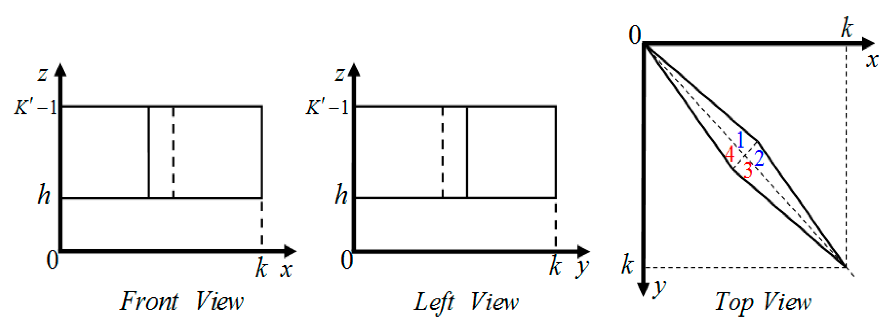
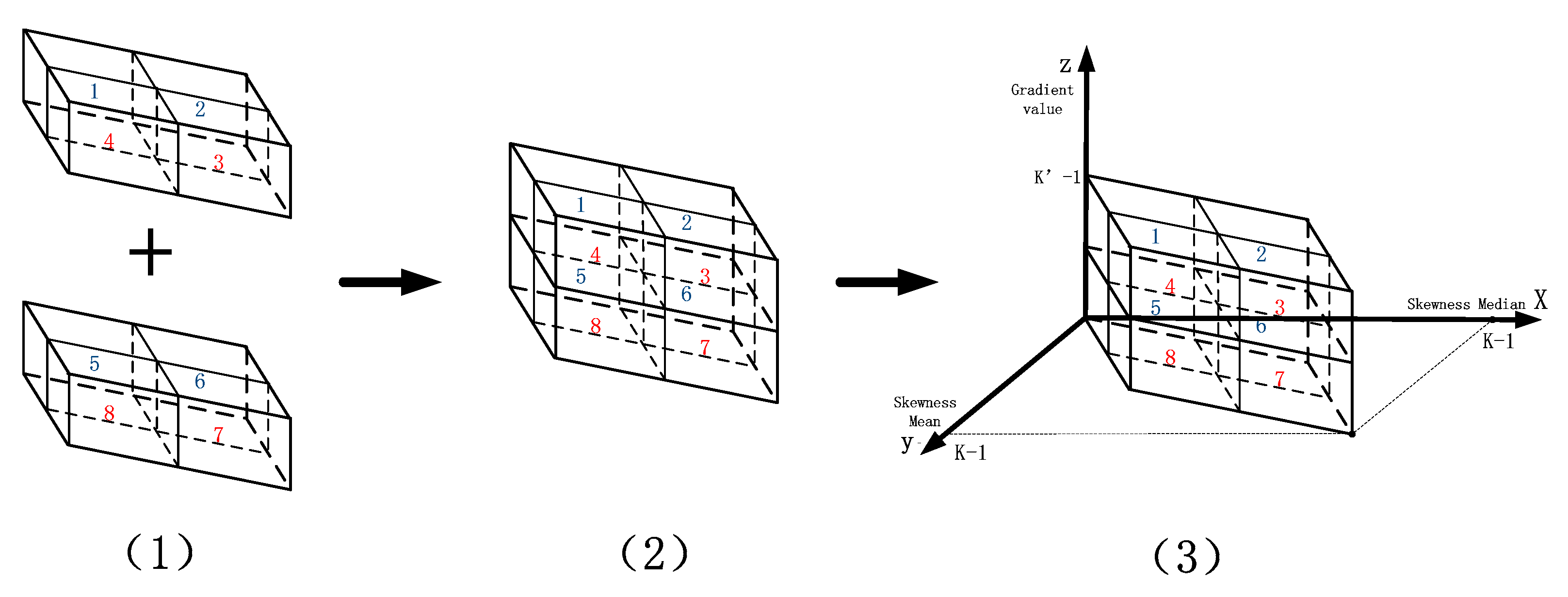
3.1. The Establishment of Three-Dimensional Information Segmentation Model

The segmentation result is not ideal due to the interpretation. In order to solve this problem, a 3D segmentation model is proposed in this paper. We considered the value of the gradient information of the contour, introduced skewness mean and skewness median value information at the same time. In addition, the paper added a median-mean filter of sub-region and sub-level for the final segmentation.

Axis Z of 3D coordinate axe expresses the image’s gradient value. While axis X and axis Y express skewness median and skewness mean. Axis X and axis Y provide the median and mean dispersion of the image’s local 3 × 3 window pixels and the entire image by skewness, which avoid the effect on image sharpness when removing the noise and return to the true image. This paper firstly calculates the sample standard dispersion ${\delta }_d$ and the mean skewness coefficient $\partial {(x)}_N$ of the 5 × 5 window pixels value. Which can be expressed as Formulas (9) and (10).

$${\delta }_d=E\left[(X_5-\mu {)}^2\right]$$

(9)

$$\partial {(x)}_N=E\left[(\frac{X_5-\mu }{{\delta }_d}{)}^3\right]+\eta$$

(10)

Therefore, Formula (11) can be obtained:

$$\begin{array}{ll}\partial (x{)}_N& =E\left[{(\frac{X_5-\mu }{{\delta }_d})}^3\right]+\eta =\frac{E\left[{(X_5-\mu )}^3\right]}{{\delta }_d{}^3}+\eta =\frac{E{X}_5{}^3-3\mu E{X}_5{}^2+3{\mu }^{2}E{X}_5-{\mu }^3}{{\delta }_d{}^3}+\eta \hfill \\ & =\frac{E{X}_5{}^3-3\mu E{X}_5{}^2+2{\mu }^3}{{\delta }_d{}^3}+\eta =\frac{E{X}_5{}^3-3E{X}_{5}E{X}_5{}^2+2E^3{X}_5}{{(E{X}_5{}^2-E^2{X}_5)}^{3/2}}+\eta \hfill \end{array}$$

(11)

In order to avoid the frequent high-power operation of window pixels, this paper simplifies as Formula (12):

$$\begin{array}{ll}\partial (x{)}_N=& E\left[{(\frac{X_5-\mu }{{\delta }_d})}^3\right]+\eta =\frac{E{X}_5{}^3-3\mu E{X}_5{}^2+3{\mu }^{2}E{X}_5-{\mu }^3}{{\delta }_d{}^3}+\eta \hfill \\ & =\frac{E{X}_5{}^3-3\mu (E{X}_5{}^2+\mu E{X}_5)-{\mu }^3}{{\delta }_d{}^3}+\eta =\frac{E{X}_5{}^3-3\mu {\delta }_d{}^2-{\mu }^3}{{\delta }_d{}^3}+\eta =\frac{{\mu }^3}{{\delta }_d{}^3}+\eta \hfill \end{array}$$

(12)

where, $X_5$ is 5 × 5 window pixels sample, $\mu$ is global mean, ${\delta }_d$ is the sample standard dispersion of window and global, $\eta$ is the skewness correction coefficient which makes the skewness coefficient greater than zero.

The skewness mean is ${\mu }_s=\partial {(x)}_N\mu$. Similarly, the skewness median $m_{gs}$ is expressed as Formulas (13) and (14).

$$\partial {(x)}_{\mathrm{M}}=E\left[{(\frac{X_5-m_g}{{\delta }_s})}^3\right]+\eta =\frac{m_g{}^3}{{\delta }_s{}^3}+\eta$$

(13)

$$m_{gs}=\partial {(x)}_M{m}_g$$

(14)

For all the pixels in the image, the target and background pixels have the largest proportion, the target area and background area within the pixel gray level is relatively uniform, the skewness mean and skewness median value of the 5 × 5 neighborhood around a pixel $i(x,y)$ are approximately equal, it usually expresses in the two-dimensional plane that the pixel value is concentrated in a narrow band on both sides of the quadrant bisector, at this time, pixels away from the bisector can be ignored. The values of the skewness coefficient are evenly distributed in the right neighborhood of origin, and the area-midpoint is the demarcation point of positive and negative skewness before revision. According to the theory of skewness values, when the mean and median of skewness are less than k/2, $m_{gs}\ge {\mu }_s$. When the mean and median of skewness are greater than k/2, $m_g{}_s\le {\mu }_s$. Thus, the two-dimensional planform of the model is shown in Figure 4.

The image after being partitioned is placed in the three-dimensional coordinate system above, and the profile of the image object can be obtained in the upper part of the three-dimensional object. In combination with the two-dimensional analysis of the coordinate system above, the contour of the object ought to distribute in the 1,3 part of the 3D object. The 3D representation of the image is shown in Figure 5 and Figure 6.

3.2. Using the Energy Theory and the Maximum Information Entropy to Fit the Contour of the Target

This part firstly introduced the concept of curve flow entropy. The contour is compared to water flowing from high place. In the equilibrium position of the lowest point (the final stop of edge line), the water flow has the minimum mechanical energy (due to friction loss and water chain reactions) and maximum kinetic energy. The mechanical energy of the water flow is the energy of the contour when it is balanced, and the kinetic energy that represents the degree of confusion is the information entropy of the edge line at this time. The exact outline of the image object can be obtained by minimum energy range under the maximum information entropy constraints.

The Snake model needs to give an initial curve near the region of interest, and then minimizes the energy function, so that the curve will deform in the image and continue to approach the target edge. The original Snakes model proposed by Kass is composed of a set of control points as Formula (15):

$$v(s)=[x(s),y(s)]s\in [0,1]$$

(15)

where, X (s) and Y (s) represent the coordinates of each control point in the image. S is the independent variable, which is based on Fourier transform. At the control point of Snakes, the energy function is defined (the relationship between the energy and the edge line) as Formula (16):

$$E_{total}={\displaystyle \underset{s}{\int }\left(\alpha {\left|\frac{\partial }{\partial s}\overline{v}\right|}^2+\beta {\left|\frac{{\partial }^2}{\partial s^2}\overline{v}\right|}^2+E_{ext}(\overline{v}(s))\right)}ds$$

(16)

where, the first item is called elastic energy, it is the modulus of the first-order derivative of the V, the second item is called bending energy, it is the modulus of second-order derivative of the V, the third is the external energy (external force). The final segmentation of the image is converted to the minimization of the energy function $E_{total}(v)$ by the variational method (the energy of the minimization of the edge).

The maximum entropy method for image segmentation using image entropy as the criterion. The aim of this method is to divide the gray histogram of the image into independent class, it makes the total entropy of each class to the maximum. A two-dimensional gray histogram is used to calculate the maximum entropy of the image.

In this paper, the process of fitting the final contour of the target is as follows (in order to facilitate the description, in this paper, the first iterative fitting procedure is mainly introduced. The rest of the process and so forth receives less attention).

(1)

Randomly select N points on the obtained contour from the pre-segmentation as the initial iteration data source $(v_{11},v_{12},v_{13},\dots ,v_{1n})$. $v_{1i}$ represents the ith pixel of the edge line and $v_{1i}$ is the ith 5 × 5 pixels window center.

(2)

Pixels belonging to the 1,3 quadrant region in $(v_{11},v_{12},v_{13},\dots ,v_{1n})$ are selected to compose the set $(v_{11},v_{12},v_{13},\dots ,v_{1k})$. $v_{11(ij)}$ expresses pixel at (i, j) in the 5 × 5 pixels window of $v_{11}$. The pixels at the same place of the 5 × 5 neighborhood of each pixel in $(v_{11},v_{12},v_{13},\dots ,v_{1k})$ reform 25 sets of k-dimensional vector. When $k\ge N/2$, calculate the flow entropy of pixel points belong to 1,3 quadrant of the three-dimensional coordinates. When $k\le N/2$, repeat (1) process.

(3)

After one calculation, the set of pixels that $(v_{11(ij)},v_{12(ij)},v_{13(ij)},\dots ,v_{1k(ij)})(1\le i,j\le 5)$ with the maximum flow entropy in the 5 × 5 neighborhood is selected as the final contour of the object.

The fitting calculation diagram is showed in Figure 7.

This paper uses the symbol $\Psi$ to represent the flow entropy. Define the pixel flow entropy formula of three-dimensional coordinate system 1,3 region. It can be expressed as Formula (17).

$$\Psi (I_{x,y,z})={\displaystyle \sum _{x=0}^{K/2}{\displaystyle \sum _{y=K/2}^K{\displaystyle \sum _{z=h}^{K^{\prime }-1}[H(I_{x,y,z})-E(I_{x,y,z})]}}}$$

(17)

The information entropy and energy terms of $I_{x,y,z}$ in the three-dimensional coordinate system are expressed on the right side of the formula. If the segmentation result is correct, then it needs to meet the condition ${\displaystyle \sum _{x=0}^{K/2}{\displaystyle \sum _{y=K/2}^K{\displaystyle \sum _{z=h}^{K^{\prime }-1}\Psi (I_{x,y,z})}}}\to Max$ at the end of the segmentation. At this point, the pixel point set has the maximum information entropy and the minimum energy term. The two terms on the right side of Formula (12) can be expressed by the Formulas (18) and (19).

$$H(I_{x,y,z})=-\sum P(I_{x,y,z})\log P(I_{x,y,z})$$

(18)

$$E(I_{x,y,z})={\phi }_1{E}_{external}(I_{x,y,z})+{\phi }_2{E}_{blending}(I_{x,y,z})+{\phi }_3{E}_{elastic}(I_{x,y,z})+\eta$$

(19)

where, $P(I_{x,y,z})$ is the probability of the pixel $I_{x,y,z}$ appearing in the 3D coordinate system. ${\phi }_1$, ${\phi }_2$, ${\phi }_3$ are weight of the energy term. ${\phi }_1$, ${\phi }_3$ have the same sign (positive or negative) and are different from ${\phi }_2$. $\eta$ is the positive and negative correction factor, which ensures that the energy term is always negative. $E_{external}(I_{x,y,z})$, $E_{blending}(I_{x,y,z})$, $E_{elastic}(I_{x,y,z})$ are external energy, bending energy and elastic properties energy of $I_{x,y,z}$.

In view of the choice of the pixel in the algorithm process (1), the energy terms can be expressed by the Formulas (20–22). According to (1), contour provides the main information of the image and the information entropy characterizes average information of the image. (2) Contour pixels have the minimum energy value. The pixel point set in the evolution of the final iteration results is determined as the edge in a maximum probability.

$$E_{external}(I_{j,k})=\alpha (s){\nu }^{″}(s)=\sqrt{{(I_{j,k}-I_{j-1,k})}^2+{(I_{j,k}-I_{j,k-1})}^2}$$

(20)

$$E_{blending}(I_{j,k})=\beta (s){\nu }^{⁗}(s)=\Vert I_{j,k}-\frac{1}{2}(v_{j(i-1)}+v_{j(i+1)})\Vert$$

(21)

$$E_{elastic}(I_{j,k})=-\nabla E_{external}=n_i(v_{ji}-I_{j,k})$$

(22)

where, $v_{j(i-1)},v_{ji},v_{j(i+1)}$ are three adjacent pixels on target contour selected by process (1) in the jth iteration process, that are center pixels of three adjacent 5 × 5 windows. $I_{j,k}$ is the pixel in the 5 × 5 neighborhood of $v_{ji}$. $t_i=\frac{v_{ji}-v_{j(i-1)}}{\Vert v_{ji}-v_{j(i-1)}\Vert }+\frac{v_{j(i+1)}-v_{ji}}{\Vert v_{j(i+1)}-v_{ji}\Vert }$, $n_i$ is the tangent vector and the normal vector between the pixels in the center of the three adjacent 5 × 5 windows. The software flow chart is shown in Figure 8.

4. Experimental Results

In order to verify the robustness and effectiveness of the proposed algorithm, this paper conducted two groups of experiments, one group through computer simulation of interference environment, the quantitative data curve is used to contrast the segmentation results of different algorithms under the different degree interference conditions. The other group segmented the physical image segmentation under different interference environments, using subjective visual comparison to contrast the segmentation results of different algorithms.

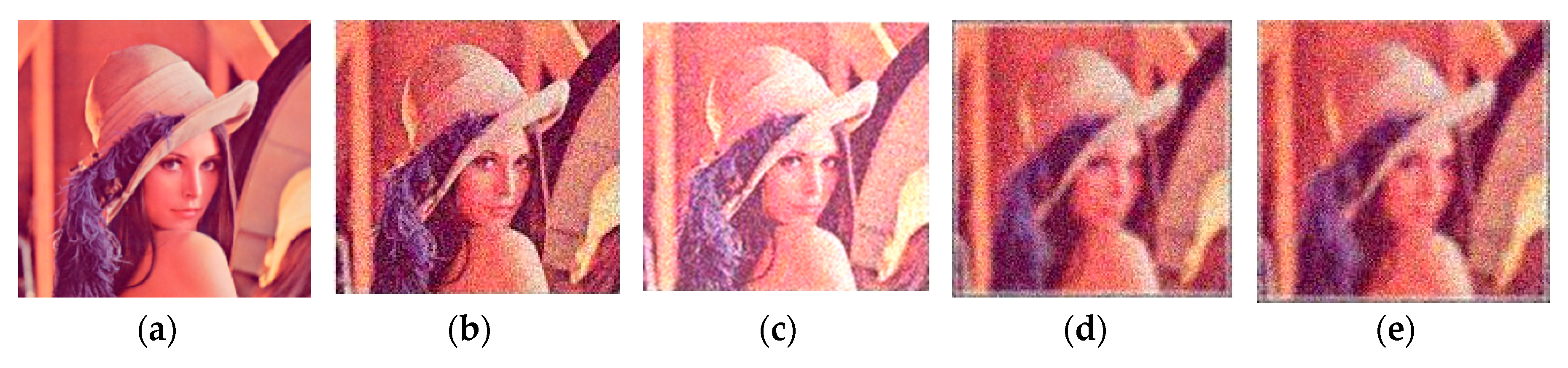
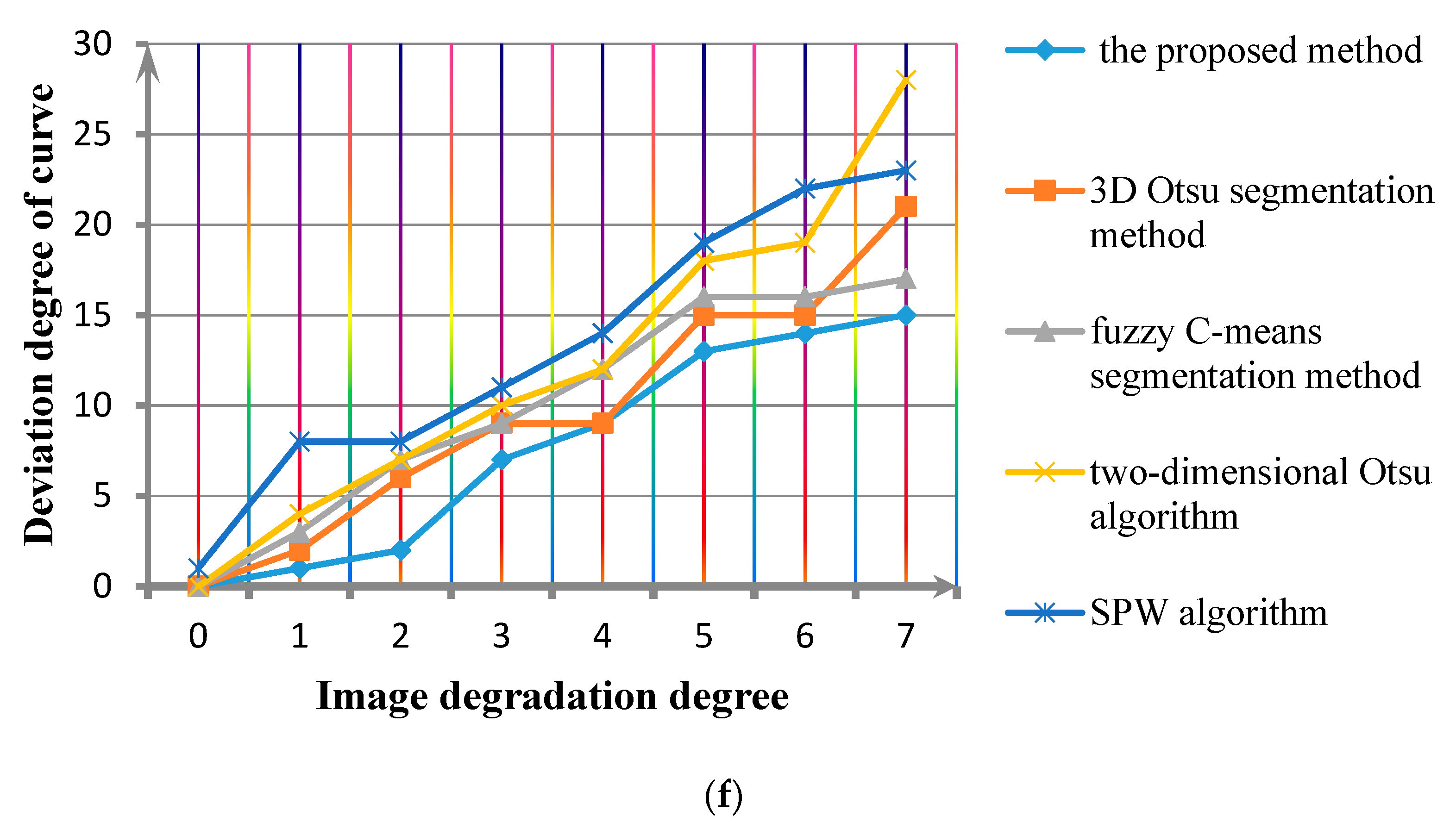
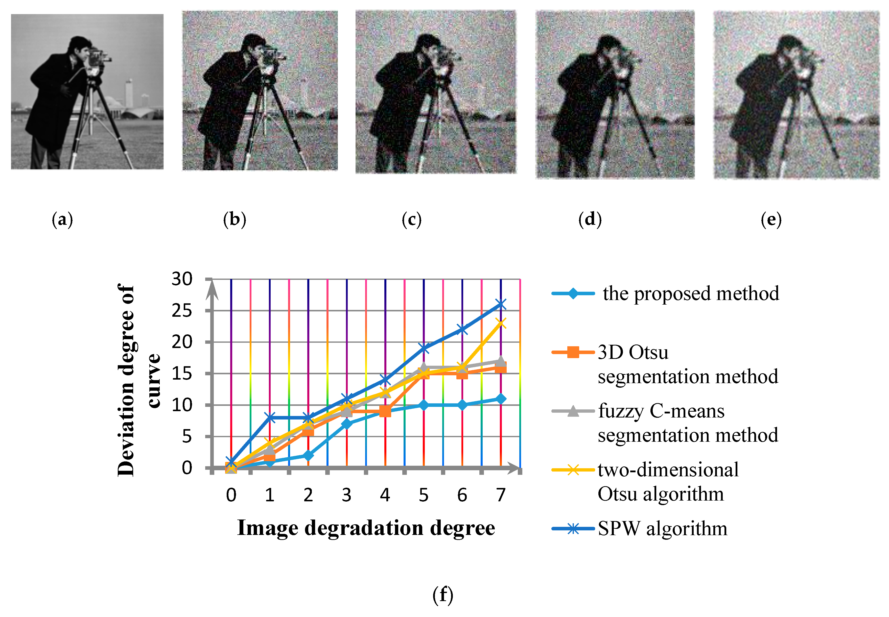
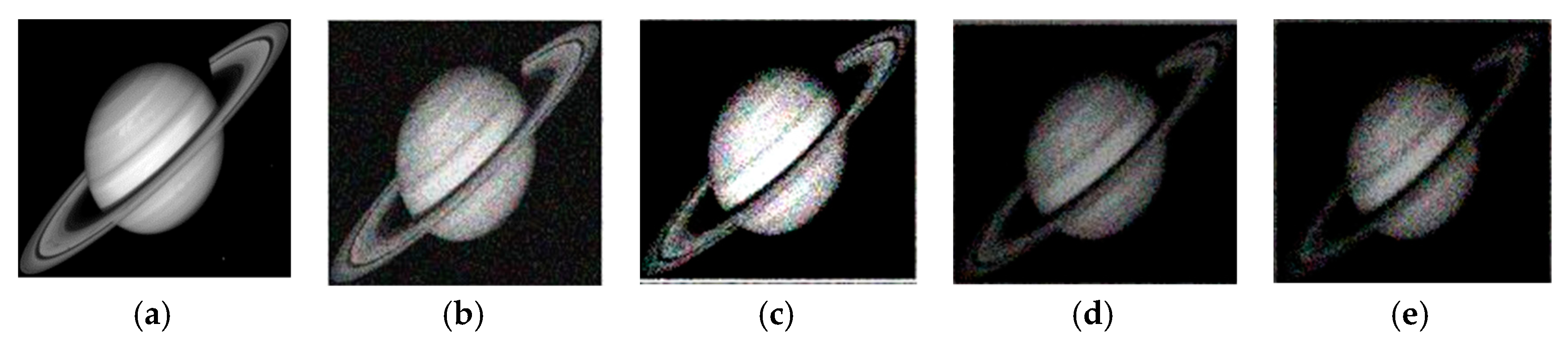
4.1. Computer Simulation Experiment

In this paper, in order to carry out simulation experiment, we first reduce the quality of the known clear image. Images of different clarity are multiplying the correlation coefficient with a constant to expand to 0–7 eight groups. The eight sets of images were labeled as $\varsigma =0$, $\varsigma =1$, $\varsigma =2$, $\varsigma =3$, $\varsigma =4$, $\varsigma =5$, $\varsigma =6$, $\varsigma =7$, where, $\varsigma$ represents the image degradation degree. In addition, the concept of a curve fit is introduced, that is, the segmentation result is judged by the similarity degree between the experimental contour of the target and the true contour of the target. In order to compare the curve fit, the closed contour of the target is expressed in function by polar coordinates. The qualitative function structure process is as shown in Figure 9.

The fit of the two curves can be expressed by the curve distance. Define zero order distance of curve in [a, b] as Formula (23).

$$d_0=\max \left|f(\rho )-\tilde{f}(\rho )\right|\rho \in [a,b]$$

(23)

where, $f(\rho )$, $\tilde{f}(\rho )$ represent real object contour function and experimental segmentation contour function.

From the curve theory, $d_0=0$ is sufficient and necessary conditions for the coincidence of the two curves. If $d_0\ne 0$, the first order distance of the two curves is still to be judged. That is Formula (24).

$$d_1=\max \left|f^{\prime }(\rho )-\widetilde{f^{\prime }}(\rho )\right|\rho \in [a,b]$$

(24)

where, $f^{\prime }(\rho )$, $\widetilde{f^{\prime }}(\rho )$ represent the first derivative real object contour function and the first derivative experimental segmentation contour function. This paper proposed the deviation degree of curve as Formula (25).

$$d=\frac{d_0+d_1}{2}$$

(25)

Comparing the segmentation experimental results with the segmentation method based on watershed transform combined an active contour model (SPW algorithm) [38], two-dimensional Otsu algorithm [39,40,41], fuzzy C-means segmentation method [42], 3D Otsu segmentation method and the proposed method, the results are shown in Figure 10, Figure 11, Figure 12 and Figure 13.

Over analysis can be obtained, comparing the segmentation experimental results with the segmentation method based on watershed transform combined with an active contour model (SPW algorithm), two-dimensional Otsu algorithm, fuzzy C-means segmentation method and 3D Otsu segmentation method. Without a fixed initial contour recognition criterion in SPW algorithm, the accuracy of the recognition results is unstable. The two-dimensional Otsu algorithm is very sensitive to noise because it is a regional threshold clustering method. When random noise appears, it will not obtain an ideal segmentation result. Fuzzy C-means algorithm’s clustering number is difficult to determine, and even when C is determined, clustering performance is still related to the selection of initial clustering centre, therefore the algorithm is very unstable. The 3D Otsu segmentation method has some anti-noise ability, but the ability of optical correction is not strong. 3D dimensional OTSU has no image pre-processing, such as uneven illumination background elimination, etc. It only considers the neighborhood gray mean value, gray mean, the image boundary information is not considered. The application of this algorithm is not wide enough. The $d$ of the proposed method is obviously minimal. That is to say, compared with other methods, the proposed method has a higher segmentation robustness for images with different definition.

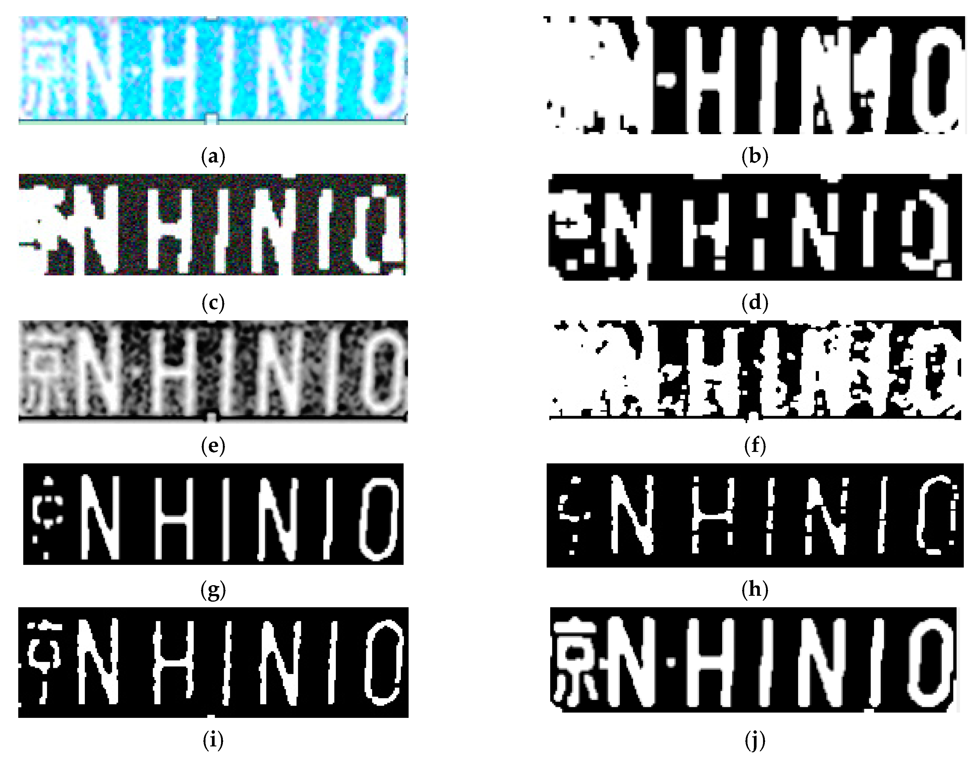
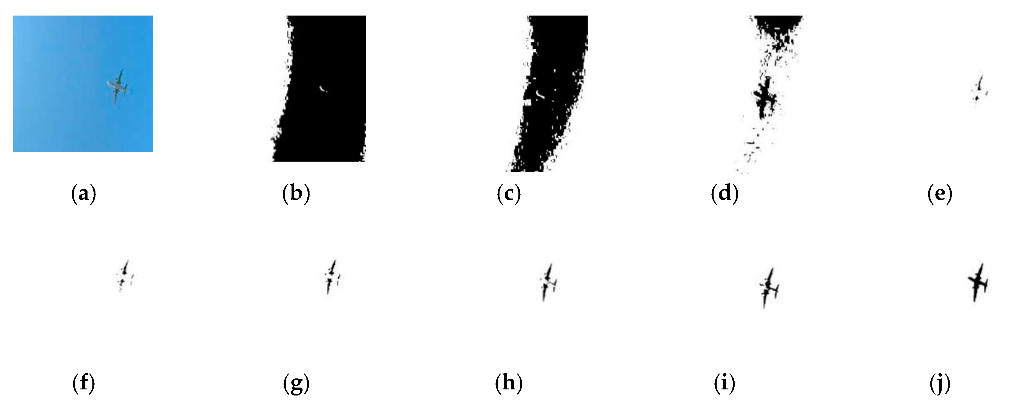
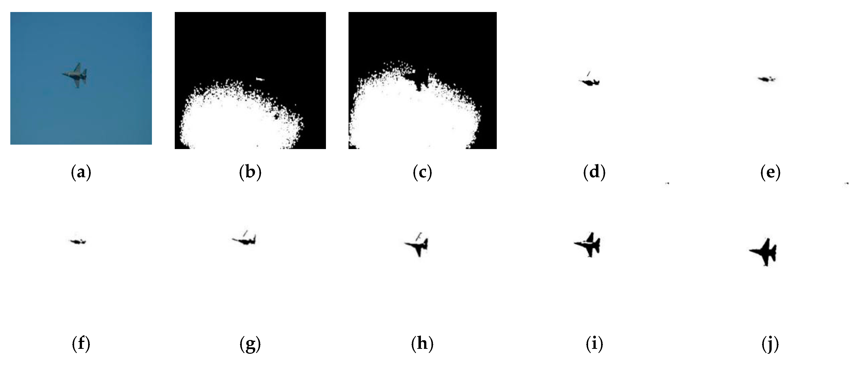
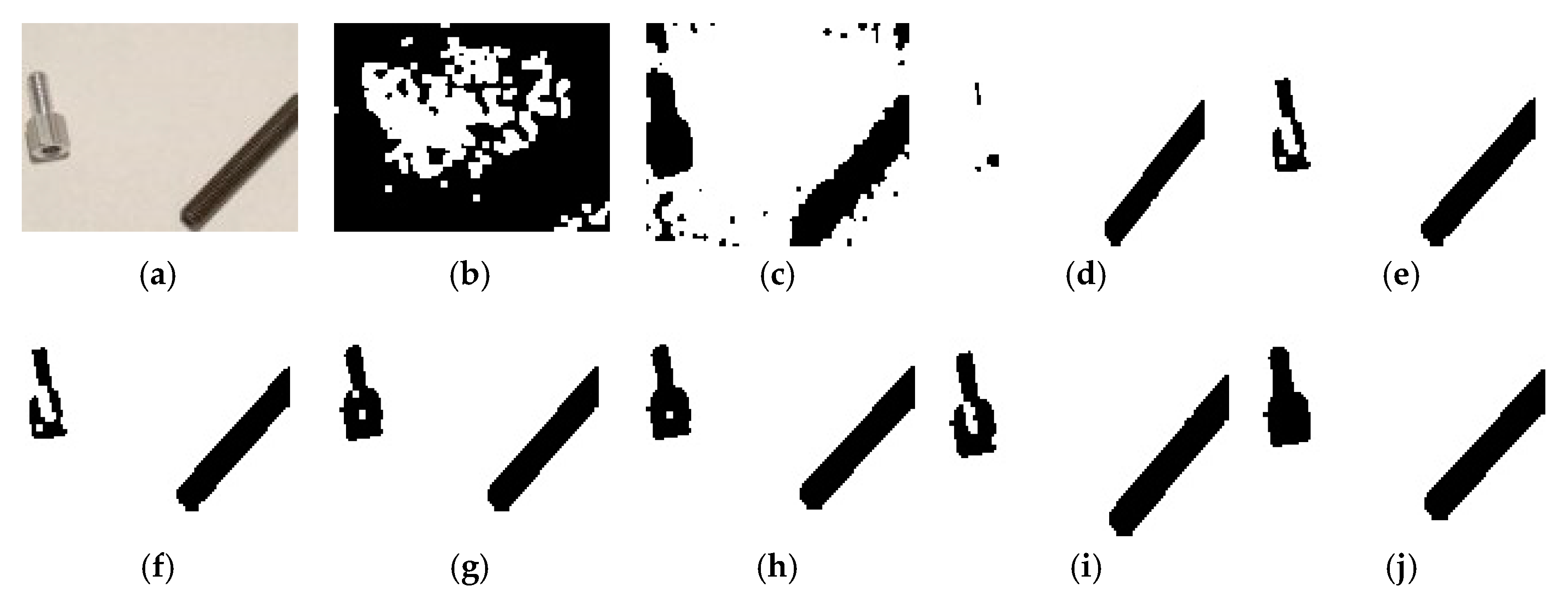
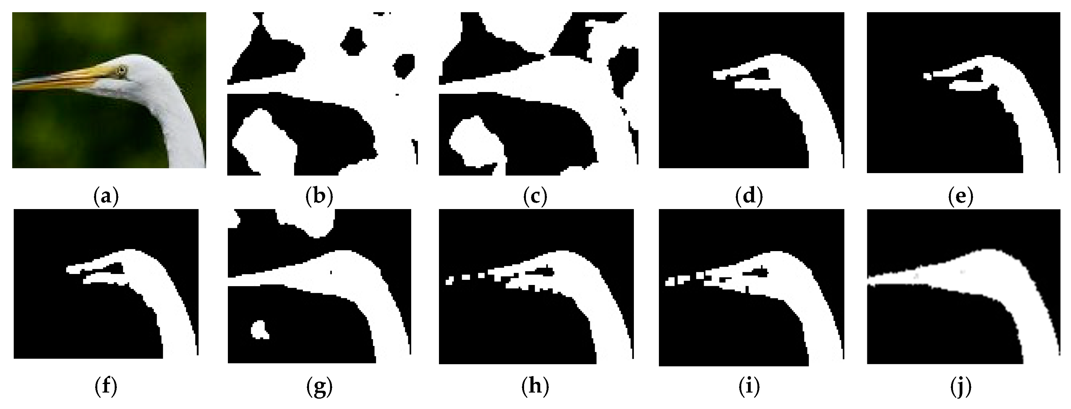
4.2. Physical Image Experiment

This paper uses seven different types of image—the license plate image under the condition of low contrast, aircraft in uneven illumination background, fighter image with low illumination, the object image with low illumination, the lighthouse image, the image of crane with rich detail information and dolphin image with local weak contrast as the experimental data. Comparing the segmentation experimental results in a segmentation method based on watershed transform combined an active contour model (SPW algorithm), two-dimensional Otsu algorithm, fuzzy C-means segmentation method, Markov Random Model of multiscale edge detection and image segmentation (MRM), the adaptive active contour method (AAC), 3D Otsu segmentation method, Semi-Supervised Learning With Deep Embedded Clustering for Image Classification and Segmentation (S’s method) [43] and Bayesian Polytrees With Learned Deep Features (BL method) [44]. The results are shown in Figure 14, Figure 15, Figure 16, Figure 17, Figure 18, Figure 19 and Figure 20.

Through the analysis of the experimental results, some conclusions can be drawn. The SPW algorithm has no normal convergence in the depressions, and the dependence of the initial contour is strong. In addition, the algorithm is not suitable for processing low contrast images. The two-dimensional Otsu algorithm effect for image preprocessing is inadequate, the algorithm is greatly influenced by noise, which impacts the segmentation results. The fuzzy C-means segmentation method is based on statistical information, segmentation of target information is not complete. In the MRM. The minimum energy configuration of the image field always corresponds to the original scene, whether in the uniform gray area or at the edge of the image. When the energy function is minimized, the MRM must distinguish whether the pixel is located at the edge. The edge detection technology is used in the segmentation algorithm. However, the edge detection operator is sensitive to noise, so the segmentation method’s anti-interference is not ideal. In the adaptive active contour method, the possibility that the active shape model converges to the local extremum is dependent on the initial edge line. If the initial contour is not well chosen, the curve may shrink to the local extremum. The convergence of the obvious concave and convex regions in the target is not ideal. In addition, the active shape model is only sampled for the pixel values in the normal direction. This normal model does not fully describe the features of the edge line. The 3D Otsu segmentation method has some anti-noise ability, but the ability of optical correction is not strong. Both of them belong to supervised in-depth learning method. S’s method and BL method, both belong to supervised deep learning-based method. They relies on a large number of training samples to learn. The selected sampling multiple and degree of confidence judging are difficult to adapt to a random background. As a result, the segmentation results are greatly affected by background interference. The proposed method has ideal pretreatment ability, combining with the advantages of threshold and energy segmentation, the segmentation effect is better than the above algorithms.

Region uniformity is used to objectively evaluate the segmentation results. It evaluates the segmentation image by calculating the uniformity degree of internal characteristics. The uniformity measure is defined as Formula (26):

$$\mathrm{UM}=1-\frac{1}{C}\sum _i\left\{\sum _{\left(x,y\right)\in R_i}{[f(x,y)-\frac{1}{A_i}\sum _{(x,y)\in R_i}f(x,y)]}^2\right\}$$

(26)

where $R_i$ is the $\mathrm{i}$-th region, and its area is $A_i$, $C$ is normalization coefficient.

Overlap measure (OM) is used to objectively evaluate the segmentation results. The accuracy of OM segmentation is the percentage of the exact segmentation area pixels in the manual signed image. OM is defined as Formula (27):

$$OM=(1-\frac{\left|R_s-T_s\right|}{R_s})\times 100\%$$

(27)

where, $R_s$ is the reference area of the true segmentation area pixels. $T_s$ is the real segmentation area pixels of the algorithm, and $\left|R_s-T_s\right|$ represents the number of pixels of the wrong segmentation.

The dice index is mainly used to calculate the similarity between two regions. The real region of the segmentation methods and the actual segmentation region of the target are taken as comparison targets. The overlapping pixels can be used as a quantitative evaluation criterion for image segmentation. The dice index is as shown in Formula (28):

$$\mathrm{Dice}=\frac{2•\left(R_{seg}\cap R_{real}\right)}{R_{seg}+R_{real}}$$

(28)

where, $R_{seg}$ is the segmentation area of the method. $R_{real}$ is the true area of the target. $R_{seg}\cap R_{real}$ is pixels of overlapping parts of the two regions. $R_{seg}+R_{real}$ is total number of pixels in two regions.

The quantitative evaluation data comparison of the five segmentation algorithms is given in

Table 1. Region uniformity comparison.

Segmentation Algorithms	License Plate Image	Aircraft Image	Fighter Image	The Object Image	The Lighthouse Image	Crane Image	Dolphin Image
The proposed method	0.9011	0.9523	0.9435	0.9501	0.8913	0.9042	0.9098
SPW	0.8016	0.4121	0.3117	0.5131	0.5962	0.6858	0.8714
2D-Otsu	0.4036	0.5271	0.4015	0.7254	0.6525	0.6555	0.8544
Fuzzy C-means	0.5542	0.4651	0.4754	0.7541	0.7288	0.7359	0.4653
MRM	0.6654	0.4553	0.4573	0.7252	0.7075	0.7459	0.4943
AAC	0.7956	0.5152	0.5565	0.7752	0.7586	0.8785	0.7789
3D-Otsu	0.8656	0.7815	0.7153	0.7963	0.8848	0.8796	0.8906
S’s method	0.8215	0.9245	0.8978	0.8645	0.8875	0.8632	0.8514
BL method	0.8773	0.8998	0.9015	0.9096	0.8563	0.8731	0.8721

,

Table 2. Overlap measure (OM) comparison.

Segmentation Algorithms	License Plate Image	Aircraft Image	Fighter Image	The Object Image	The Lighthouse Image	Crane Image	Dolphin Image
The proposed method	92.11%	94.54%	90.87%	95.52%	89.15%	90.95%	84.11%
SPW	82.16%	37.65%	44.65%	55.27%	54.89%	60.27%	64.98%
2D-Otsu	57.14%	45.15%	45.63%	60.16%	63.86%	59.88%	55.48%
Fuzzy C-means	53.16%	36.19%	59.61%	68.15%	73.02%	65.19%	57.46%
MRM	59.15%	63.03%	55.30%	65.48%	65.53%	59.05%	45.89%
AAC	47.51%	53.43%	57.15%	56.57%	69.51%	60.12%	65.88%
3D-Otsu	80.19%	77.64%	79.65%	80.22%	83.91%	87.51%	79.81%
S’s method	84.54%	89.89%	82.05%	83.79%	86.13%	81.15%	81.03%
BL method	85.13%	89.25%	81.25%	85.94%	80.82%	84.12%	80.09%

and

Table 3. Dice comparison.

Segmentation Algorithms	License Plate Image	Aircraft Image	Fighter Image	The Object Image	The Lighthouse Image	Crane Image	Dolphin Image
The proposed method	0.91	0.92	0.89	0.95	0.89	0.90	0.84
SPW	0.65	0.74	0.75	0.55	0.54	0.60	0.64
2D-Otsu	0.57	0.66	0.70	0.60	0.63	0.59	0.55
Fuzzy C-means	0.53	0.58	0.61	0.68	0.73	0.65	0.57
MRM	0.59	0.65	0.55	0.64	0.61	0.59	0.46
AAC	0.48	0.56	0.54	0.56	0.62	0.60	0.66
3D-Otsu	0.80	0.78	0.83	0.80	0.81	0.86	0.77
S’s method	0.82	0.88	0.80	0.81	0.85	0.84	0.80
BL method	0.81	0.85	0.85	0.83	0.86	0.81	0.81

. The greater the uniformity measure, in OM and dice, the better the segmentation result would be. As shown in the Table 1, Table 2 and Table 3, the dependence of the initial contour in SPW algorithm is strong and the result has a randomness. 2D-Otsu is greatly affected by noise, and cannot effectively segment the image seriously polluted by noise. Due to the clustering’s uncertainties, Fuzzy C-means cannot cluster accurately when segmenting the noise polluted image and the low-contrast image, causing serious error-segmentation. But it has a strong robustness to the slow uneven illumination change. MRM’s anti-interference is not ideal, the uniformity measure of MRM is low under the condition of interference. AAC converges to multiple local regions in the process of convergence of target initial edge line. In the uniform area, the convergence effect of edge line is ideal. However, in the obvious concave and convex parts of targets, the convergence of edges tends to be wrong. The 3D-Otsu algorithm has good anti-noise performance, but gets undesirable results in dark area if the segmentation basis coefficient is not appropriately chosen. S’s method and the BL method are the deep learning based methods, they are able to more accurately grasp the boundaries and regions of interested objects, but are limited by the supervised training of the sample set, they are easily disturbed by complex environments when using network to determine the confidence of targets. On the contrary, the proposed algorithm in this paper achieved an outstanding segmentation result on noise-polluted, low-contrast, and multiple targets and uneven illumination change.

We also give the comparison of the calculation times among the proposed method with other methods presented in this paper, and the results are shown in

Table 4. Running time of the four methods on test images (s).

Segmentation Algorithms	License Plate Image	Aircraft Image	Fighter Image	The Object Image	The Lighthouse Image	Crane Image	Dolphin Image
the proposed algorithm	9.25	9.19	8.97	8.98	9.01	9.19	8.49
SPW	8.17	8.81	8.74	7.25	7.19	8.57	8.23
2D-Otsu	4.72	5.23	6.16	3.29	4.64	4.52	5.54
Fuzzy C-means	7.64	8.05	8.01	7.59	7.03	6.98	8.45
MRM	9.12	9.36	10.14	11.73	9.69	9.42	10.57
AAC	8.97	8.14	8.02	5.95	6.14	7.59	8.42
3D-Otsu	10.12	12.14	9.69	11.37	12.49	10.91	9.56
S’s method	8.98	9.19	8.39	8.19	8.19	8.94	9.11
BL method	8.17	8.29	9.01	8.55	9.14	9.33	9.67

. In this paper, the computer hardware configuration used by the algorithm execution is: CPU is i3-380, the main frequency is 2 GHz, the internal memory is 1G, and the software environment is Matlab7.0.

We carried out the calculation of the complexity of the algorithm. In order to express it intuitively, we firstly classified the method of the upper table. The SPW method and the AAC method belong to the way of the energy contour line iteration. The computational efficiency of the algorithm is mainly determined by the convergence speed of the discrete contour energy function. 2D-Otsu, Fuzzy C-means, MRM and are the threshold segmentation method. The computational efficiency of the 2D-Otsu is mainly determined by the calculation of the similarity distance between classes. The computational efficiency of the Fuzzy C-means is mainly determined by the calculation of the optimal central threshold. The computational efficiency of the MRM is mainly determined by the calculation of the number of layers in the Markov model and the optimal threshold for each layer. The computational efficiency of the 3D-Otsu is mainly determined by the calculation of iterative solution of the three-dimensional distance. The similarity between the initial segmentation classes (Complexity O(n)) and the execution time of the 3D flow entropy comparison (Complexity O(n²)) determines the computational efficiency of the proposed method. There is no uniform computational complexity in the deep learning based method, and the operation time of image segmentation can be obtained according to the connection design of the network.

5. Conclusions and Future Works

The proposed 3D flow of the entropy contour fitting segmentation algorithm based on the multi-scale transform contour constraint, within the scope of the initial contour line, considers the gradient information of the image, regional skewness mean and skewness median information. When a 3D coordinate is established, a simplified algorithm based on moment theory and a novel flow entropy segmentation method is used in determining the contour. The experimental results prove that the algorithm has an ideal segmentation effect for images. Because of the algorithm still uses an iterative method, operation speed does not substantially improve. In the future, it needs to improve the operation process of the existing algorithm, and further reduce the running time of the algorithm.

References

1. Qi, C.M. Maximum entropy for image segmentation based on an adaptive particle swarm optimization. Appl. Math. Inf. Sci. 2014, 8, 3129–3135. [Google Scholar] [CrossRef]
2. Ahmed, L.J.; Jeyakumar, A.E. Image segmentation using a refined comprehensive learning particle swarm optimizer for maximum tsallis entropy thresholding. Int. J. Eng. Technol. 2013, 5, 3608–3616. [Google Scholar]
3. Lu, Y.; Zhao, W.; Mao, X. Multi-threshold image segmentation based on improved particle swarm optimization and maximum entropy method. Adv. Mater. Res. 2014, 12, 3649–3653. [Google Scholar] [CrossRef]
4. Filho, P.P.R.; Cortez, P.C.; da Silva Barros, A.C.; de Albuquerque, V.H.C. Novel Adaptive Balloon Active Contour Method based on internal force for image segmentation—A systematic evaluation on synthetic and real images. Expert Syst. Appl. 2014, 41, 7707–7721. [Google Scholar] [CrossRef]
5. Li, D.; Li, W.; Liao, Q. A fuzzy geometric active contour method for image segmentation. IEICE Trans. Inf. Syst. 2013. [Google Scholar] [CrossRef]
6. Padmapriya, B.; Kesavamurthi, T. An approach to the calculation of volume of urinary bladder by applying localising region-based active contour segmentation method. Int. J. Biomed. Eng. Technol. 2013, 13, 177–184. [Google Scholar] [CrossRef]
7. Li, M.; Yang, H.; Zhang, J.; Zhou, T.; Tan, Z. Image thresholding segmentation research based on an improved region division of two-dimensional histogram. J. Optoelectron. Laser 2013, 24, 1426–1433. [Google Scholar]
8. Fan, J.L.; Zhao, F.; Zhang, X.F. Recursive algorithm for three-dimensional Otsu’s thresholding segmentation method. Acta Electron. Sin. 2017, 35, 1398–1402. [Google Scholar]
9. Gao, L.; Yang, S.; Li, H. New unsupervised image segmentation via marker-based watershed. J. Image Graph. 2017, 12, 1025–1032. [Google Scholar]
10. Liang, H.; Jia, H.; Xing, Z.; Ma, J.; Peng, X. Modified grasshopper algorithm-based multilevel thresholding for color image segmentation. IEEE Access 2019, 12, 11258–11295. [Google Scholar] [CrossRef]
11. Rapaka, S.; Kumar, P.R. Efficient approach for non-ideal iris segmentation using improved particle swarm optimisation-based multilevel thresholding and geodesic active contours. IET Image Process. 2018, 12, 1721–1729. [Google Scholar] [CrossRef]
12. Zhang, C.; Xie, Y.; Liu, D.; Wang, L. Fast threshold image segmentation based on 2D fuzzy fisher and random local optimized QPSO. IEEE Trans. Image Process. 2017, 26, 1355–1362. [Google Scholar] [CrossRef] [PubMed]
13. Li, Q.; Zheng, M.; Li, F.; Wang, J.; Geng, Y.; Jiang, H. Retinal image segmentation using double-scale non-linear thresholding on vessel support regions. CAAI Trans. Intell. Technol. 2017, 2, 109–115. [Google Scholar] [CrossRef]
14. Zheng, L.; Li, G.; Jiang, H. Improvement of the gray image maximum entropy segmentation method. Comput. Eng. Sci. 2010, 32, 53–56. [Google Scholar]
15. Wu, J.; Zhang, Y.; Bai, J.; Weng, W.; Wu, Y.; Han, Y.; Li, J. Tongue contour image extraction using a watershed transform and an active contour model. J. Tsinghua Univ. (Sci. Technol.) 2018, 48, 1040–1043. [Google Scholar]
16. Arbelaez, P.; Maire, M.; Fowlkes, C.; Malik, J. Contour detection and hierarchical image segmentation. IEEE Trans. Pattern Anal. Mach. Intell. 2011, 33, 898–916. [Google Scholar] [CrossRef] [PubMed]
17. Li, L.; Zhou, F.; Bai, X. Infrared pedestrian segmentation through background likelihood and object-biased saliency. IEEE Trans. Intell. Transp. Syst. 2018, 19, 2826–2844. [Google Scholar] [CrossRef]
18. Chen, B.; Qiu, F.; Wu, B. Image segmentation based on constrained spectral variance difference and edge penalty. Remote Sens. 2015, 7, 5980–6004. [Google Scholar] [CrossRef]
19. Montoya, M.; Gil, C.; Garcia, I. The load unbalancing problem for region growing image segmentation algorithms. J. Parallel Distrib. Comput. 2003, 63, 387–395. [Google Scholar] [CrossRef]
20. Haris, K.; Efstratiadis, S.; Maglaveras, N. Hybrid image segmentation using watersheds and fast region merging. IEEE Trans. Image Process. 1998, 7, 1684–1699. [Google Scholar] [CrossRef] [Green Version]
21. Soille, P. Constrained connectivity for hierarchical image partitioning and simplification. IEEE Trans. Pattern Anal. Mach. Intell. 2018, 30, 1132–1145. [Google Scholar] [CrossRef] [PubMed]
22. Ma, B.; Ban, X.; Huang, H.; Chen, Y.; Liu, W.; Zhi, Y. Deep learning-based image segmentation for Al-La alloy microscopic images. Symmetry 2018, 10, 107. [Google Scholar] [CrossRef]
23. Badrinarayanan, V.; Kendall, A.; Cipolla, R. SegNet: A deep convolutional encoder-decoder architecture for image segmentation. IEEE Trans. Pattern Anal. Mach. Intell. 2017, 39, 2481–2495. [Google Scholar] [CrossRef] [PubMed]
24. Minaee, S.; Wang, Y. Screen content image segmentation using least absolute deviation fitting. In Proceedings of the 2015 IEEE International Conference on Image Processing (ICIP), Quebec City, QC, Canada, 27–30 September 2015; pp. 3295–3299. [Google Scholar]
25. Chen, L.; Yang, Y.; Wang, J.; Xu, W.; Yuille, A.L. Attention to scale: Scale-aware semantic image segmentation. In Proceedings of the 2016 IEEE Conference on Computer Vision and Pattern Recognition (CVPR), Las Vegas, NV, USA, 27–30 June 2016; pp. 3640–3649. [Google Scholar]
26. van Opbroek, A.; Achterberg, H.C.; Vernooij, M.W.; de Bruijne, M. Transfer learning for image segmentation by combining image weighting and kernel learning. IEEE Trans. Med Imaging 2019, 38, 213–224. [Google Scholar] [CrossRef] [PubMed]
27. Chen, L.C.; Papandreou, G.; Schroff, F.; Adam, H. Rethinking atrous convolution for semantic image segmentation. Comput. Vis. Pattern Recognit. 2017, 12, 210–217. [Google Scholar]
28. Minaee, S.; Wang, Y. An ADMM approach to masked signal decomposition using subspace representation. IEEE Trans. Image Process. 2019, 28, 3192–3204. [Google Scholar] [CrossRef]
29. Braquelaire, J.P.; Brun, L. Image segmentation with topological maps and inter-pixel representation. J. Vis. Commun. Image Represent. 1998, 9, 62–79. [Google Scholar] [CrossRef]
30. Arbelaez, P.A.; Cohen, L.D. Energy partitions and image segmentation. J. Math. Imaging Vis. 2004, 20, 43–57. [Google Scholar] [CrossRef]
31. Amelio, A.; Pizzuti, C. An evolutionary approach for image segmentation. Evol. Comput. 2014, 22, 525–557. [Google Scholar] [CrossRef]
32. Wang, X.; Wan, S.; Lei, T. Brain tumor segmentation based on structuring element map modification and marker-controlled watershed transform. J. Softw. 2014, 9, 2925. [Google Scholar] [CrossRef]
33. Saini, S.; Arora, K.S. Enhancement of watershed transform using edge detector operator. Int. J. Eng. Sci. Res. Technol. 2014, 3, 763–767. [Google Scholar]
34. Zhang, J.; Hou, H.; Zhao, X. A modified Otsu segmentation algorithm based on preprocessing by Top-hat transformation. Sens. World 2011, 17, 9–11. [Google Scholar]
35. Liu, R.; Peng, Y.; Tang, C.; Cheng, S. Object auto-segmentation based on watershed and graph cut. J. Beijing Univ. Aeronaut. Astronaut. 2012, 38, 636–640. [Google Scholar]
36. Zhu, S. Function extension and application of morphological top-hat transformation and bottom-hat transformation. Comput. Eng. Appl. 2011, 47, 190–192. [Google Scholar]
37. Ge, W.; Gao, L.Q.; Shi, Z.G. An algorithm based on wavelet lifting transform for extraction of multi-scale edge. J. Northeast. Univ. (Nat. Sci.) 2017, 4, 3005–3026. [Google Scholar]
38. Claveau, V.; Lefèvre, S. Topic segmentation of TV-streams by watershed transform and vectorization. Comput. Speech Lang. 2015, 29, 63–80. [Google Scholar] [CrossRef] [Green Version]
39. Chen, Q.; Zhao, L.; Lu, J.; Kuang, G. Modified two-dimensional Otsu image segmentation algorithm and fast realization. IET Image Process. 2012, 6, 426–433. [Google Scholar] [CrossRef]
40. Nakib, A.; Oulhadj, H.; Siarry, P. A thresholding method based on two-dimensional fractional differentiation. Image Vis. Comput. 2009, 27, 1343–1357. [Google Scholar] [CrossRef]
41. Guo, W.; Wang, X.; Xia, X. Two-dimensional Otsu’s thresholding segmentation method based on grid box filter. Optik 2014, 125, 5234–5240. [Google Scholar] [CrossRef]
42. Zhang, W.; Kang, J. Neighboring weighted fuzzy C-Means with kernel method for image segmentation and its application. Optik 2013, 13, 2306–2310. [Google Scholar]
43. Enguehard, J.; Halloran, P.; Gholipour, A. Semi-supervised learning with deep embedded clustering for image classification and segmentation. IEEE Access 2019, 3, 11093–11104. [Google Scholar] [CrossRef]
44. Fehri, H.; Gooya, A.; Lu, Y.; Meijering, E.; Johnston, S.A.; Frangi, A.F. Bayesian polytrees with learned deep features for multi-class cell segmentation. IEEE Trans. Image Process. 2019, 28, 3246–3260. [Google Scholar] [CrossRef] [PubMed]
Figure 1. Schematic diagram of circular base structure.
Symmetry 11 00857 g001
Figure 2. Image preprocessing. (a) Initial image, (b) Original background image, (c) Results of traditional top-hat and bottom-hat transform, (d) Gauss filter processing results, (e) Wavelet transform enhancement results, (f) Algorithm processing results of this paper.
Symmetry 11 00857 g002
Figure 3. Comparison results of initial contour detection. (a) Initial image, (b) watershed segmentation, (c) The proposed method.
Symmetry 11 00857 g003
Figure 4. The two-dimensional model of the mean and median of skewness.
Symmetry 11 00857 g004
Figure 5. Schematic diagram of the three views of the upper part of the image’s 3D object.
Symmetry 11 00857 g005
Figure 6. Schematic diagram of image’s 3D structure combination.
Symmetry 11 00857 g006
Figure 7. Sketch map of the first outline fitting calculation.
Symmetry 11 00857 g007
Figure 8. Schematic diagram of software flow.
Symmetry 11 00857 g008
Figure 9. The qualitative function structure process.
Symmetry 11 00857 g009
Figure 10. Lena noise simulation image and experimental result curve. (a) ς = 0 , (b) ς = 1 , (c) ς = 3 , (d) ς = 5 , (e) ς = 7 , (f) The evaluation index curve.
Symmetry 11 00857 g010aSymmetry 11 00857 g010b
Figure 11. Cameraman noise simulation image and experimental result curve. (a) ς = 0 , (b) ς = 1 , (c) ς = 3 , (d) ς = 5 , (e) ς = 7 , (f) The evaluation index curve.
Symmetry 11 00857 g011
Figure 12. Saturn noise simulation image and experimental result curve. (a) ς = 0 , (b) ς = 1 , (c) ς = 3 , (d) ς = 5 , (e) ς = 7 , (f) The evaluation index curve.
Symmetry 11 00857 g012aSymmetry 11 00857 g012b
Figure 13. Cell noise simulation image and experimental result curve. (a) ς = 0 , (b) ς = 1 , (c) ς = 3 , (d) ς = 5 , (e) ς = 7 , (f) The evaluation index curve.
Symmetry 11 00857 g013
Figure 14. Segmentation results of license plate image under low contrast condition. (a) Original image, (b) SPW algorithm, (c) Two-dimensional OTSU algorithm, (d) Fuzzy C-mean algorithm, (e) Markov Random Model of multiscale edge detection and image segmentation (MRM), (f) adaptive active contour method (AAC), (g) 3D OTSU algorithm, (h) Semi-Supervised Learning With Deep Embedded Clustering for Image Classification and Segmentation (S’s) method, (i) Bayesian Polytrees With Learned Deep Features (BL) method, (j) The proposed method.
Symmetry 11 00857 g014
Figure 15. Segmentation results of aircraft in uneven illumination background. (a) Original image, (b) SPW algorithm, (c) Two-dimensional OTSU algorithm, (d) Fuzzy C-mean algorithm, (e) MRM, (f) AAC, (g) 3D OTSU algorithm, (h) S’s method, (i) BL method, (j) The proposed method.
Symmetry 11 00857 g015
Figure 16. Segmentation results of fighter image under low illumination. (a) Original image, (b) SPW algorithm, (c) Two-dimensional OTSU algorithm, (d) Fuzzy C-mean algorithm, (e) MRM, (f)AAC, (g) 3D OTSU algorithm, (h) S’s method, (i) BL method, (j) The proposed method.
Symmetry 11 00857 g016
Figure 17. The segmentation results of the object image. (a) Original image, (b) SPW algorithm, (c) Two-dimensional OTSU algorithm, (d) Fuzzy C-mean algorithm, (e) MRM, (f) AAC, (g) 3D OTSU algorithm, (h) S’s method, (i) BL method, (j) The proposed method.
Symmetry 11 00857 g017
Figure 18. The segmentation results of the Lighthouse image. (a) Original image, (b) SPW algorithm, (c) Two-dimensional OTSU algorithm, (d) Fuzzy C-mean algorithm, (e) MRM, (f) AAC, (g) 3D OTSU algorithm, (h) S’s method, (i) BL method, (j) The proposed method.
Symmetry 11 00857 g018
Figure 19. The segmentation results of crane. (a) Original image, (b) SPW algorithm, (c) Two-dimensional OTSU algorithm, (d) Fuzzy C-mean algorithm, (e) MRM, (f) AAC, (g) 3D OTSU algorithm, (h) S’s method, (i) BL method, (j) The proposed method.
Symmetry 11 00857 g019
Figure 20. The segmentation results of dolphin image with local weak contrast. (a) Original image, (b) SPW algorithm, (c) Two-dimensional OTSU algorithm, (d) Fuzzy C-mean algorithm, (e) MRM, (f) AAC, (g) 3D OTSU algorithm, (h) S’s method, (i) BL method, (j) The proposed method.
Symmetry 11 00857 g020