Article

Fixed Coeficient A(α) Stable Block Backward Differentiation Formulas for Stiff Ordinary Differential Equations

by
Zarina Bibi Ibrahim
1,*,
Nursyazwani Mohd Noor
2 and
Khairil Iskandar Othman
3
1
Institute for Mathematical Research, Department of Mathematics, Faculty of Science, Universiti Putra Malaysia, Serdang 43400, Selangor, Malaysia
2
Department of Mathematics, Faculty of Science, Universiti Putra Malaysia, Serdang 43400, Selangor, Malaysia
3
Department of Mathematics, Faculty of Computer and Mathematical Sciences, Universiti Teknologi MARA, Shah Alam 40450, Selangor, Malaysia
*
Author to whom correspondence should be addressed.
Symmetry 2019, 11(7), 846; https://doi.org/10.3390/sym11070846
Submission received: 27 March 2019 / Revised: 27 May 2019 / Accepted: 27 May 2019 / Published: 1 July 2019

Abstract

:
The main contribution in this paper is to construct an implicit fixed coefficient Block Backward Differentiation Formulas denoted as A ( α ) -BBDF with equal intervals for solving stiff ordinary differential equations (ODEs). To avoid calculating the differentiation coefficients at each step of the integration, the coefficients of the formulas will be stored, with the intention of optimizing the performance in terms of precision and computational time. The plots of their A ( α ) stability region are provided, and the order of the method is also verified. The necessary conditions for convergence, such as the consistency and zero stability of the method, are also discussed. The numerical results clearly showed the efficiency of the method in terms of accuracy and execution time as compared to other existing methods in the scientific literature.

1. Introduction

Ordinary Differential Equations (ODEs) are frequently used in much mathematical modelling of real-world problems. Many of the applications, notably in chemical engineering and control theory, exhibit a phenomenon known as stiffness (see [1]). As stated by [2], stiff systems are found in the description of atmospheric phenomena, chemical reactions occurring in living species, chemical kinetics (e.g., explosions), engineering control systems, electronic circuits, lasers, mechanics and molecular dynamics. Many factors, such as stability, step size selection, precision, and computer time, should be taken into account when developing a numerical method for stiff ODEs. The requirement on A-stability puts a severe limitation on the choice of suitable methods for the solution of stiff ODEs (see [3,4]). Therefore, a great deal of effort focuses on the development of numerical methods with a larger stability region with the property of A-stability, so as to cope with the ‘stiffness’ of the differential equations. The concept of A-stability for initial value problems in ODEs was introduced by [5]. Dahlquist proved that the trapezoidal method has the highest order (=2) of the global discretization error term and has the smallest error constant of all linear A-stable multistep methods.
In this paper, we consider general first order ordinary differential equations of the following form:
y ( x ) = f ( x , y ( x ) ) ,   y ( a ) = y 0 ,   a x b
where y = f ( x , y ) is a real valued function in the interval [ a , b ] , which satisfies the Lipschitz conditions that assured the existence and uniqueness of the solution to Equation (1). The phenomenon of stiffness is not precisely defined in the literature. It is most common to define stiffness in terms of the eigenvalues of the Jacobian matrix. Equation (1) is said to be stiff if the eigenvalues λ i ( x ) of the Jacobian matrix f / y satisfy the following conditions:
  • R e a l ( λ i ( x ) ) < 0 , i = 1 , 2 , , n
  • max t | R e a l ( λ i ( x ) ) | min t | R e a l ( λ i ( x ) ) |
The development of multistep block methods for solving Equation (1) has been studied by many researchers (see [3,5,6,7,8,9,10,11]). Recently, numerous works have focused on the modification of various types of multistep block methods to improve the efficiency in terms of the accuracy of the approximate solution and the computational time, (see [3,5,6,7,8,9,10,11]). Although many block multistep methods have been introduced in the past, most of these methods are based on Adams formulas for solving the ODEs, and the focus is specifically on the solution of non-stiff systems of ODEs. For the solution of stiff ODEs, the challenge is to develop a suitable implicit method with A-stability properties. It is important to develop an accurate algorithm with good stability properties since it is well known that stability appears to be the most serious limitation of block methods [12].
Backward Differentiation Formulas (BDFs) have been widely used due to their good stability properties. Many block methods based on the classical BDFs have been proposed for stiff ODEs. Among the most popular block methods based on Backward Differentiation Formulas (BDFs) are the Block Backward Differentiation Formulas (BBDFs) (see [8,11,12]). They proposed an r-point Block Backward Differentiation Formula (r-BBDF), which was later extended by [13,14,15]. It was reported that the block method based on BDF can be very effective in solving stiff ODEs in terms of reducing the computational time and improving the accuracy of the approximate solution [6,7,8,9,10,11,13,14,15]. Motivated by the fact that the work that was conducted based on BDF is efficient in solving stiff ODEs, our aim is to construct and perform some modifications to the existing block BDF by extending the method to produce three approximate solutions at a single iteration.
The paper is organized as follows; in Section 2, we present the derivation of the method, followed by a discussion on the stability of the method in Section 3. The implementation of the method will be discussed in Section 4, followed by the numerical results for the new methods in Section 5. Finally, the conclusions will be presented in Section 6.

2. Derivation of the Method

In this section, the new implicit fixed coefficient Block Backward Differentiation Formulas, denoted as A ( α ) -BBDF, are constructed with equal intervals. These block methods will generate three approximate solutions simultaneously at a single iteration from the values generated in the last block, as described by [7]. [16] took a similar approach in adjusting the BBDF given in [7] by introducing future points and the extra parameter ρ . The major setback of the method by [16] is choosing the best value for the parameter ρ when developing the coefficients of the correctors. Thus, the coefficient for the new formulas will be computed by choosing a better value for the parameter ρ in order to improve the stability intervals and also the accuracy of the approximate solution. Moreover, the value of ρ is chosen from the given interval ( 1 , 1 ) . A detailed description of the parameter ρ for the solution of Equation (1) can be found in many publications [16,17].
Assuming that the solution values y n 2 ,   y n 1 , and y n , specified as back values, are available, the new three-point A ( α ) -BBDF method which defines the next block of approximations y n + 1 ,   y n + 2 , and y n + 3 will be derived. First, we consider the following k-step linear multistep method (LMM) as defined in [18]:
j = 0 k α j y n + j = h j = 0 k β j f n + j
where α j and β j are unknown constants which must be determined, and k is the step number of the method employed, and also assuming that α k 0 and that α 0 and β 0 are not both equal to zero. The method in Equation (2) is explicit when β k = 0 and implicit otherwise. We have followed the LMM as defined in Equation (2) by specifying the following conditions, which include the free parameter ρ . The general form of an implicit method with k equally spaced points for solving Equation (1) can be expressed as:
j = 0 k α j , i   y n + j 2 = h β i ( f n + i ρ f n + i 1 ) ,   i = 1 , 2 , 3
so that the coefficients to be defined in Equation (3) satisfy the condition of A-stability. In Equation (3), α j , i and β i are the coefficient matrixes of y n and f n that must be computed, and ρ is a free parameter chosen in the interval ( 1 , 1 ) , as specified in [16]. From our numerical experiments, ρ = 7 / 8 is chosen since it gives good stability properties required for solving stiff ODEs. The value ρ = 7 / 8 was successfully substituted into Equation (3). Specifying k = 5 , the linear difference operator L i , associated with the linear multistep method, is given as follows:
L i [ y ( x n ) ; h ] = j = 0 5 α j , i y n + j 2 h β i ( f n + i + 7 8 f n + i 1 ) .
Now, we expand Equation (4) to obtain:
L i [ y ( x n ) ; h ] = α 0 , i y n 2 + α 1 , i y n 1 + α 2 , i y n + α 3 , i y n + 1 + α 4 , i y n + 2 + α 5 , i y n + 3 h β i ( f n + 1 + 7 8 f n + i 1 ) = α 0 , i y ( x n 2 h ) + α 1 , i y ( x n h ) + α 2 , i y ( x n ) + α 3 , i y ( x n + h ) + α 4 , i y ( x n + 2 h ) +   α 5 , i y ( x n + 3 h ) h β i ( f ( x n + i h ) + 7 8 f ( x n + ( i 1 ) h ) ) = α 0 , i y ( x n 2 h ) + α 1 , i y ( x n h ) + α 2 , i y ( x n ) + α 3 , i y ( x n + h ) + α 4 , i y ( x n + 2 h ) +   α 5 , i y ( x n + 3 h ) h β i ( f ( x n + i h ) + 7 8 f ( x n + ( i 1 ) h ) )
where i = 1 , 2 , 3 . Expanding by the Taylor series about x = x n , we obtain the following:
α j , i y ( x n + ( j 2 ) h ) = α j , i [ y ( x n ) + ( j 2 ) h y ( x n ) + ( ( j 2 ) h ) 2 2 ! y ( x n ) + ( ( j 2 ) h ) 3 3 ! y ( x n ) + ] ,
β i f ( x n + ( i 1 ) h ) = β i [ y ( x n ) + ( i 1 ) h y ( x n ) + ( ( i 1 ) h ) 2 2 ! y ( x n ) + ( ( i 1 ) h ) 3 3 ! y ( 4 ) ( x n ) + ]
β i f ( x n + i h ) = β i [ y ( x n ) + i h y ( x n ) + ( i h ) 2 2 ! y ( x n ) + ( i h ) 3 3 ! y ( 4 ) ( x n ) + ] .
Then, collecting the terms in y n and its derivatives, we obtain the following equation:
L i [ y ( x n ) ; h ] = C 0 , i y ( x n ) + C 1 , i h y ( x n ) + C 2 , i h 2 y ( x n ) + C 3 , i h 3 y ( x n ) + + C q , i h q y ( q ) = 0
where
C 0 , i = α 0 , i + α 1 , i + α 2 , i + α 3 , i + α 4 , i + α 5 , i
C 1 , i = 2 α 0 , i α 1 , i + α 3 , i + 2 α 4 , i + 3 α 5 , i β i ( 1 ρ )
C q , i = 1 q ! ( ( 2 ) q α 0 , i + ( 1 ) q α 1 , i + α 3 , i + 2 q α 4 , i + 3 q α 5 , i ) β i ( i ( q 1 ) ( q 1 ) ! ρ ( i 1 ) q 1 ( q 1 ) ! )
with q = 2 , 3 .
The coefficients of α j , i and β i are determined by substituting α 3 , 1 , α 4 , 2 , α 5 , 3 = 1 into Equation (6) for i = 1 , 2 , 3 . The resulting equations will be solved simultaneously, and the results are tabulated in Table 1.
All the values in Table 1 are substituted into Equation (5). Hence, the corresponding formulas for A ( α ) -BBDF take the following form:
y n + 1 = 1 116 y n 2 + 9 58 y n 1 + 31 29 y n 27 116 y n + 2 + 1 58 y n + 3 + 21 29 h f n + 24 29 h f n + 1 y n + 2 = 1 73 y n 2 + 11 146 y n 1     6 73 y n + 82 73 y n + 1 15 146 y n + 3 + 43 73 h f n + 1 + 48 73 h f n + 2 y n + 3 =       15 236 y n 2 23 59 y n 1   +     y n 78 59 y n + 1 + 389 236 y n + 2 + 21 59 h f n + 2 + 24 59 h f n + 3 }

2.1. Order of the Method

In Section 2.1, the order of the proposed method will be verified. We illustrate the definitions of the order for the Linear Multistep Method (LMM) as given in [18], using the following LMM Equation (2) and the associated difference operator L, defined by:
L [ z ( x ) ; h ] = j = 0 k [ α j z ( x + j h ) h β j z ( x + j h ) ]
are said to be of the order p if C 0 = C 1 = = C p = 0 ,   C p + 1 0 . The general form for the constant C q is defined as:
C q = j = 0 k [ 1 q ! j q α j 1 ( q 1 ) ! j q 1 β j ] ,   q = 2 , 3 , , p + 1 .
Since the derived method is a block method, we extend the definition given in Equation (9) in the following form:
L [ z ( x ) ; h ] = j = 0 k [ A j z ( x + j h ) h B j z ( x + j h ) ]
where Aj and Bj are r by r matrices. Note that the constant Cq can be rewritten as:
C q = j = 0 k [ 1 q ! j q A j 1 ( q 1 ) ! j q 1 B j ] ,   q = 2 , 3 , , p + 1 .
It is easily shown that:
C 6 = j = 0 5 [ 1 6 ! j 6 A j 1 5 ! j 5 B j ] = [ 1 / 580 9 / 730 33 / 590 ] [ 0 0 0 ]
The term C 6 represents the error constant of the method. Since C 0 = C 1 = = C 5 = 0 , we conclude that the order of the developed method is five.

3. Stability Analysis

In this section, we will investigate the linear stability analysis for the derived method. This will lead to the location of the roots of the associated stability polynomial with respect to the unit circle in the complex plane.

3.1. Zero Stability

The standard definition of zero stability for block methods assumes the following definition introduced by Fatunla [19].
Definition 1.
The block method is zero stable provided the roots R j , j = 1 ( 1 ) k of the first characteristic polynomial
γ ( r ) = det [ i = 0 k A i R k i ] = 0 ,   A ( 0 ) = I
satisfy | R j | 1 , and that for those roots with | R j | = 1 , the multiplicity must not exceed 1. The principal root of γ ( r ) is denoted by R 1 = R 2 = 1 . A ( i ) ,   i = 0 ( 1 ) k are r by r matrices.
We start by considering the following test equation:
y = λ y
where λ is a complex number with a negative real part. We substitute Equation (11) into Equation (8) to obtain the matrix coefficients specified as:
A = [ 1 24 29 h ¯ 27 116 1 58 82 73 42 73 h ¯ 1 48 73 h ¯ 15 146 78 59 389 236 21 59 h ¯ 1 24 59 h ¯ ] , B = [ 1 116 9 58 31 29 + 21 29 h ¯ 1 73 11 146 6 73 15 236 23 59 1 ]
with h ¯ = h λ . We have the stability polynomial of the method by computing d e t ( A t B ) . The stability polynomial is given as follows:
514809 999224 t 399 999224 h ¯ 765 499612 + 1452159 999224 t 3 594477 249806 t 2 h ¯ 2 1002297 499612 t 3 h ¯ + 132399 124903 t 3 h ¯ 2 27648 124903 t 3 h ¯ 3 + 24507 124903 t h ¯ 2 18522 124903 t 2 h ¯ 3 + 70407 124903 t h ¯ 982719 499612 t 2 1379493 999224 t 2 h ¯
Substituting h ¯ = 0 in Equation (12), we solve the following equation to determine the roots of the stability polynomial:
1452159 999224 t 3 982719 499612 t 2 + 514809 999224 t 765 499612   = 0
Thus, we have the roots t = 1 ,   0.0030 , and 0.3504 . Since | t | 1 , we conclude that the method is zero stable.

3.2. Stability Region

The region of absolute stability is the set of points h λ for which the method produces a solution that never increases in magnitude, i.e., | y n + 1 | | y n | (see [20]). The chosen step size h should lie within the region of absolute stability of the numerical method.
Definition 2.
A numerical method is A-stable if its region of absolute stability contains the whole left-hand half-plane R e ( h λ ) < 0 , as illustrated in Figure 1. The stability region is denoted by the shaded areas.
Unfortunately for LMM, the A-stable methods cannot have an order greater than 2, as stated in [20]. Furthermore, an explicit LMM cannot be A stable (see [20]). The weakening of this property leads to the following definition (see [20]).
Definition 3.
A method is stiffly stable with a stiffness abscissa D if the stability region includes all complex numbers z such that R e ( z ) D .
Definition 4.
A method is A ( α ) stable if the stability region includes all complex numbers such that ( π α ) a r g ( z ) π α .
Definition 5.
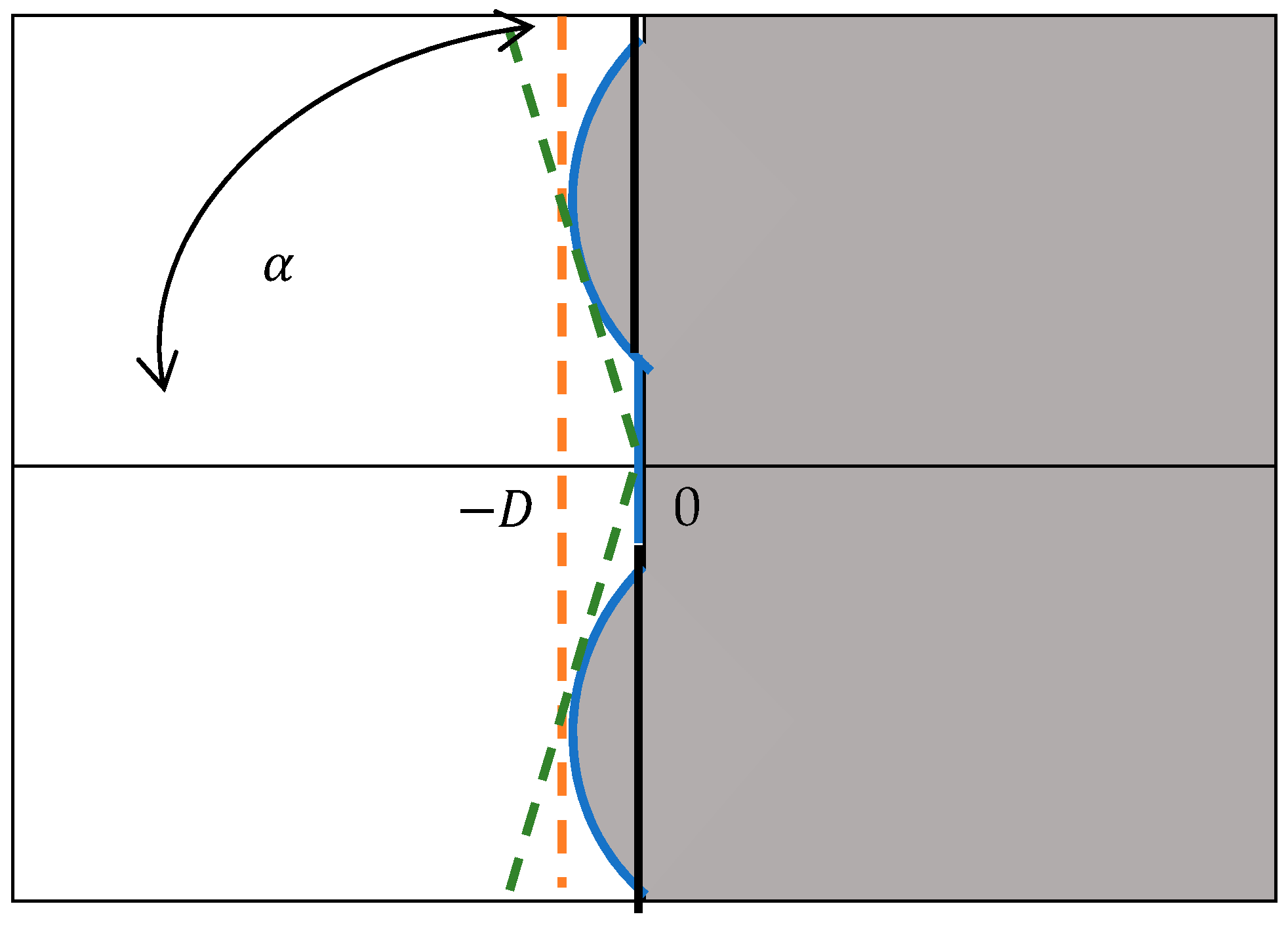
is illustrated in Figure 2 by using a Backward Differentiation Formula of order 4, (BDF4), as an example. For BDF4, α = 73.352 ° and D = 0.66667 .
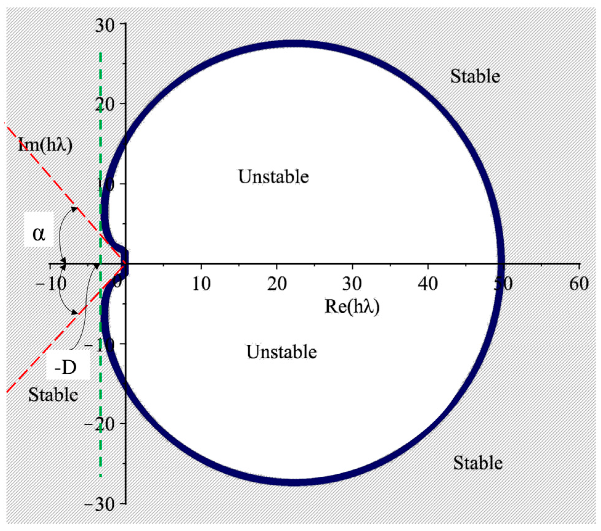
The boundary of the stability region is given by the set of points determined by t i θ , 0 θ 2 π , for which | t | 1 . Thus, the stability region of A ( α ) -BBDF, with α = 49.057 ° and D = 2.723 , is shown in Figure 2. The region of absolute stability lies outside the boundary.
It can clearly be seen in Figure 3 that our new method in Equation (8) is A ( α ) stable, as defined in [20]. Next, we discuss the convergence associated with the method in Equation (2).

3.3. Convergence of the Method

The necessary conditions for the convergence of the new method are determined using a theorem taken from [18], which states that a linear multistep method is convergent if and only if it is zero stable and consistent. The LMM given in Equation (2) is consistent if it satisfies these two conditions:
  • j = 0 k α j = 0
  • j = 0 k j α j = j = 0 k β j
Based on these conditions, we determined the consistency of the formulas given in Equation (2). We obtained:
  • j = 0 5 A j = [ α 0 , 1 α 0 , 2 α 0 , 3 ] + [ α 1 , 1 α 1 , 2 α 1 , 3 ] + [ α 2 , 1 α 2 , 2 α 2 , 3 ] + [ α 3 , 1 α 3 , 2 α 3 , 3 ] + [ α 4 , 1 α 4 , 2 α 4 , 3 ] + [ α 5 , 1 α 5 , 2 α 5 , 3 ]   = [ 1 116 1 73 15 236 ] + [ 9 58 11 146 23 59 ] + [ 31 29 6 73 1 ] + [ 1 82 73 78 59 ] + [ 27 116 1 389 236 ] + [ 1 58 15 146 1 ] = [ 0 0 0 ] .
  • j = 0 5 j A j = ( 0 ) [ α 0 , 1 α 0 , 2 α 0 , 3 ] + ( 1 ) [ α 1 , 1 α 1 , 2 α 1 , 3 ] + ( 2 ) [ α 2 , 1 α 2 , 2 α 2 , 3 ] + ( 3 ) [ α 3 , 1 α 3 , 2 α 3 , 3 ] + ( 4 ) [ α 4 , 1 α 4 , 2 α 4 , 3 ] + ( 5 ) [ α 5 , 1 α 5 , 2 α 5 , 3 ] = ( 0 ) [ 1 116 1 73 15 236 ] + ( 1 ) [ 9 58 11 146 23 59 ] + ( 2 ) [ 31 29 6 73 1 ] + ( 3 ) [ 1 82 73 78 59 ] + ( 4 ) [ 27 116 1 389 236 ] + ( 5 ) [ 1 58 15 146 1 ] = [ 45 29 90 73 45 59 ] = j = 0 5 B j .
We have shown that the conditions given in [18] are satisfied. Therefore, we have verified that the A ( α ) -BBDF in Equation (8) converged.

4. Implementation

For the implementation of the method, the code developed for the A ( α ) -BBDF method would perform the scheme referred to as the PECE mode (Predict, Evaluate, Correct, Evaluate). The following illustrates how the derived method is implemented to solve Equation (1).
Step 1. 
Predict: y n + 1 p ,   y n + 2 p ,   y n + 3 p are developed explicitly.
Step 2. 
Evaluate: f n + 1 = f ( x n + 1 , y n + 1 p )
f n + 2 = f ( x n + 2 , y n + 2 p )
f n + 3 = f ( x n + 3 , y n + 3 p )
Step 3. 
Correct: y n + 1 ,   y n + 2 , y n + 3 by
Step 4. 
Evaluate: f n + 1 = f ( x n + 1 , y n + 1 )
f n + 2 = f ( x n + 2 , y n + 2 )
f n + 3 = f ( x n + 3 , y n + 3 )
The major drawback in the implementation of the A ( α ) -BBDF in general is that they are not self starting. In this case, the Euler method is used for the computation of the backvalues. Hence, Equation (8) can be solved using Newton’s iteration, and we restrict the number of iterations to two, i.e.,
Y n + j ( i + 1 ) Y n + j ( i ) = [ F j ( y n + j ( i ) ) ] 1 [ F j ( y n + j ( i ) ) ] ,   j = 1 , 2 , 3
where
F 1 = y n + 1 + 27 116 y n + 2 1 58 y n + 3 21 29 h f n 24 29 h f n + 1 ς 1
F 2 = y n + 2 82 73 y n + 1 + 15 146 y n + 3 42 73 h f n + 1 48 73 h f n + 2 ς 2
F 3 = y n + 3 + 78 59 y n + 1 389 236 y n + 2 21 59 h f n + 2 24 59 h f n + 3 ς 3
ς 1 ,   ς 2 and ς 3 are the backvalues, given as follows:
ς 1 = 1 116 y n 2 + 9 58 y n 1
ς 2 = 1 73 y n 2 + 11 146 y n 1
ς 3 = 15 236 y n 2 23 59 y n 1
The notation i is introduced to specify the iteration. Thus, y n + 1 ( i + 1 ) will denote the i th iterative value of y n + 1 , and e n + 1 ( i + 1 ) =   y n + 1 ( i + 1 ) y n + 1 ( i ) will denote the differences between the i th and ( i + 1 ) th iterative values of y n + 1 . Similarly y n + 2 ( i + 1 ) will denote the i th iterative value of y n + 2 , and y n + 3 ( i + 1 ) will denote the i th iterative value of y n + 3 . Thus,
e n + 1 , n + 2 , n + 3 ( i + 1 ) = y n + 1 , n + 2 , n + 3 ( i + 1 ) y n + 1 , n + 2 , n + 3 ( i )
The following computations, written in matrix form, are carried out to obtain the approximations:
[ 1 24 29 h f n + 1 y n + 1 27 116 1 58 82 73 42 73 h f n + 1 y n + 1 1 48 73 h f n + 2 y n + 2 15 146 78 59 389 236 21 59 h f n + 2 y n + 2 1 24 59 h f n + 3 y n + 3 ] [ e n + 1 ( i + 1 ) e n + 2 ( i + 1 ) e n + 3 ( i + 1 ) ] = [ 1 27 116 1 58 82 73 1 15 146 78 59 389 236 1 ] [ y n + 1 ( i ) y n + 2 ( i ) y n + 3 ( i ) ] + h [ 0 0 21 29 0 0 0 0 0 0 ] [ f n 2 ( i ) f n 1 ( i ) f n ( i ) ] + h [ 24 29 0 0 42 73 48 73 0 0 21 59 24 59 ] [ f n + 1 ( i ) f n + 2 ( i ) f n + 3 ( i ) ] + [ ς 1 ς 2 ς 3 ]

5. Numerical Results

In order to show the performance of the A ( α ) -BBDF method, the code was tested on several problems, three of which are presented in this paper. It seems appropriate to compare the new method with the existing method of the same order. We consider numerical solutions using the following three methods:
  • The fifth order method given by [12].
  • The fifth order method derived by [13].
  • The new A ( α ) -BBDF.
    Problem 1:
    y = 20 ( y x 2 ) + 2 x with initial value y ( 0 ) = 1 / 3 and x [ 0 , 1 ]
    Exact solution: y ( x ) = x 2 + 1 3 e 20 x
    Source: Burden and Faires [21].
    Problem 2:
    y = y ( 1 y ) 2 y 1 with initial value y ( 0 ) = 5 / 9 and x [ 0 , 5 ]
    Exact solution: y ( x ) = 1 2 + 1 4 5 36 e x
    Source: Alvarez and Rojo [22].
    Problem 3:
    y 1 = 21 y 1 + 19 y 2 20 y 3
    y 2 = 19 y 1 21 y 2 20 y 3
    y 3 = 40 y 1 40 y 2 40 y 3
    y 1 ( 0 ) = 1 ,   y 2 ( 0 ) = 0 ,   y 3 ( 0 ) = 1   ,   x [ 0 , 1 ]
    Exact solution:
    y 1 ( x ) = 0.5 [ e 2 x + e ( 40 + 40 i ) x ]
    y 2 ( x ) = 0.5 [ e 2 x e ( 40 + 40 i ) x ]
    y 3 ( x ) = e ( 40 + 40 i ) x
    Source: Lambert [18].
Table 2, Table 3 and Table 4 shows the numerical results for Problems 1 to 3. We use the following abbreviations:
BBDF(5):Fifth order Block Backward Differentiation Formula in [12]
3SBBDF:3-point Superclass of Block Backward Differentiation Formula in [14]
A ( α ) -BBDF:New 3-point BBDF
NS:Number of steps
h :Step size
T:Computing time in seconds
MAXE:Maximum error
The maximum error is defined as
MAXE   =   max 0 n N S | y ( x ) y n ( x ) |
where y ( x ) is the exact solution, and y ( x n ) is the computed solution.
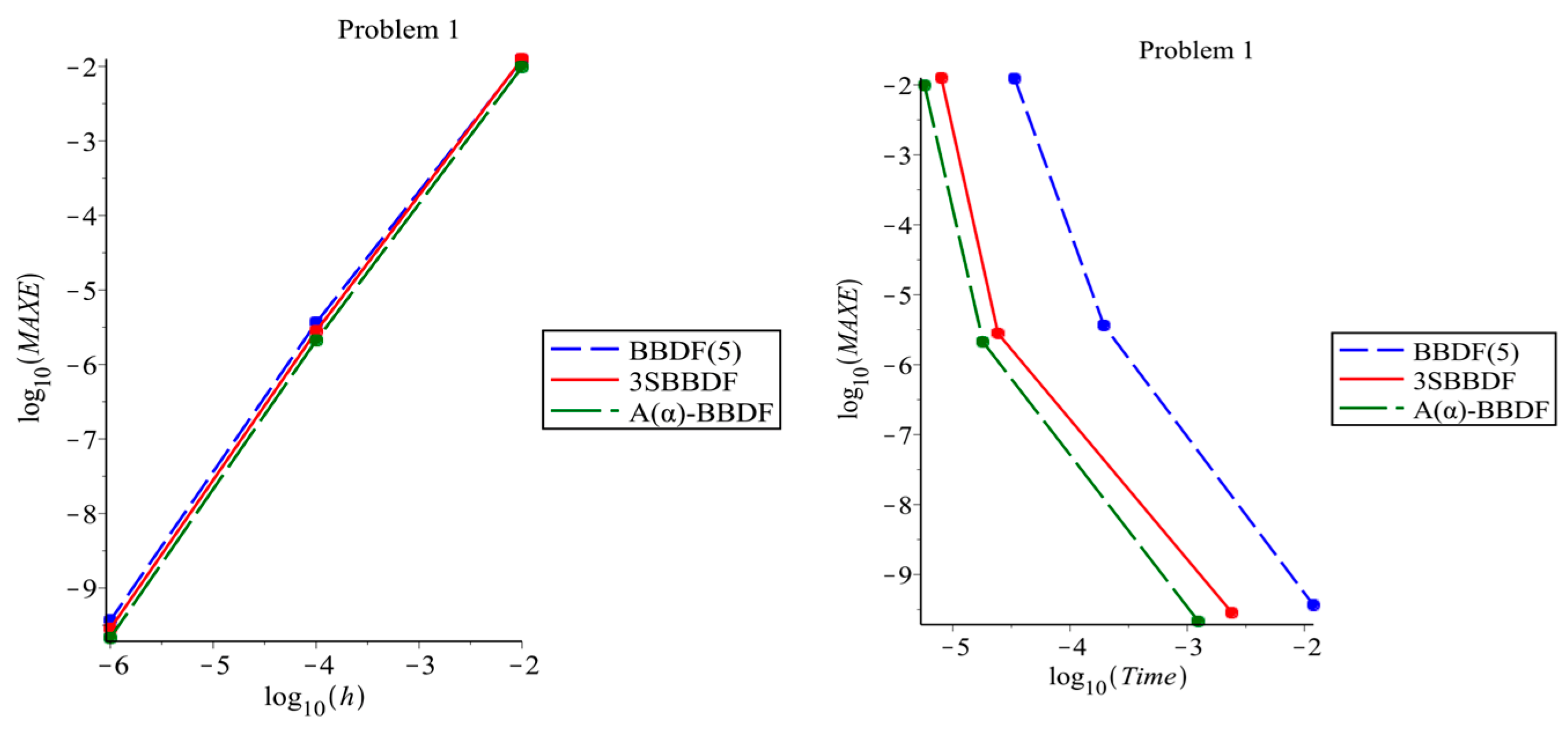
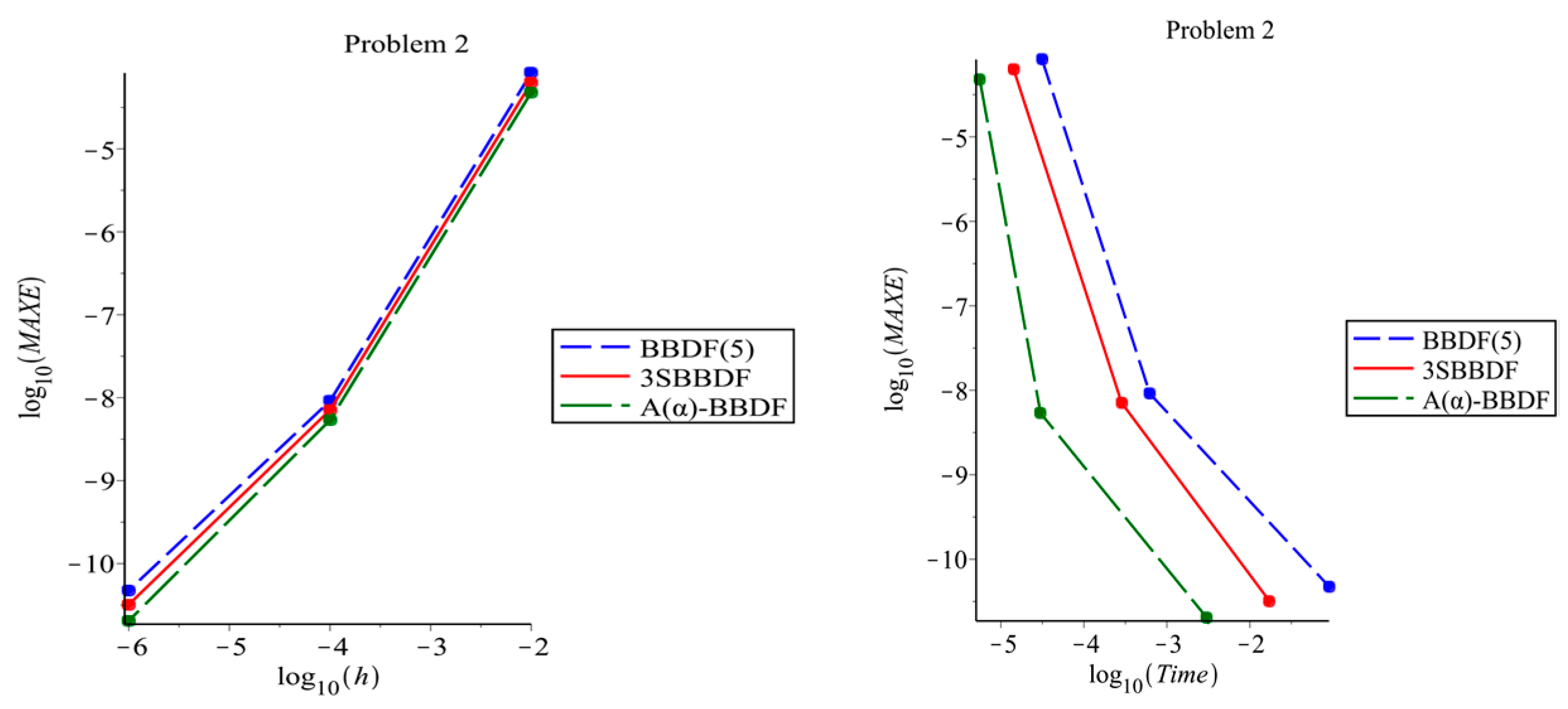
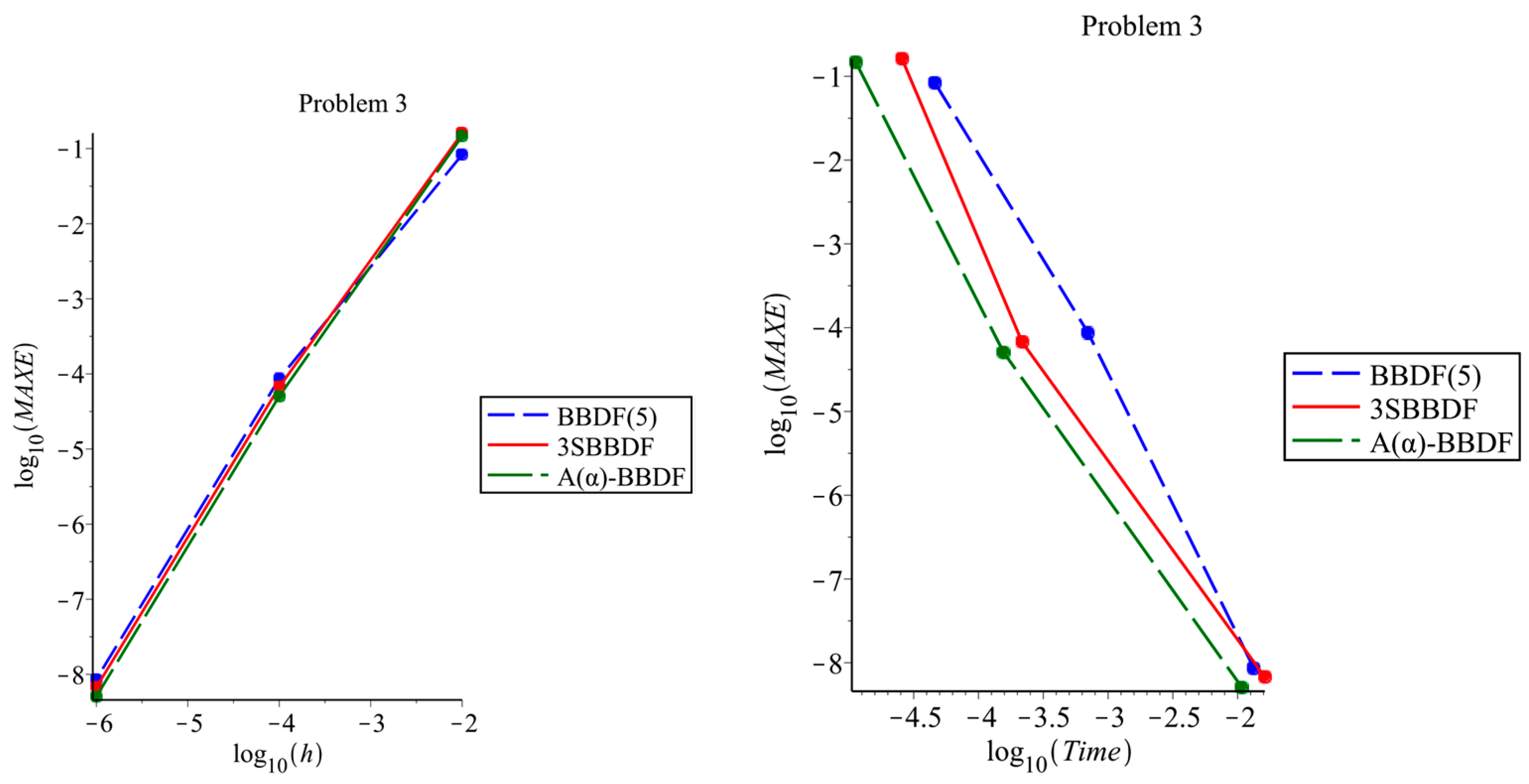
The following figures show the relation between the maximum error and computational time for Problems 1 to 3 at various step sizes.
Figure 4, Figure 5 and Figure 6 show the variations of the step size with different errors in the A ( α ) -BBDF method. It can be seen that, when using A ( α ) -BBDF, a lower computational time is needed to achieve the same degree of accuracy when compared to BBDF(5) and 3SBBDF.

6. Discussion and Conclusions

In this paper, we construct the implicit A ( α ) -BBDF of order five to solve first order ODEs. The method is based on the classical BDF but differs in terms of the numbers of approximate solutions produced at each step of the integration. In our case, three approximate solutions are produced simultaneously at each step of the integration. These will facilitate a parallel implementation in the future. The numerical results support the efficiency of the new A ( α ) -BBDF method in terms of increasing the degree of accuracy with less computational time. Therefore, the derived method can be a suitable alternative for solving stiff ODEs.

Author Contributions

Conceptualization, Z.B.I.; Methodology, Z.B.I., N.M.N.; Investigation, N.M.N.; resources, K.I.O.; Writing—original draft preparation, Z.B.I.; N.M.N.; Writing—review and editing, Z.B.I., K.I.O.; Visualization, N.M.N.; supervision, Z.B.I.; project administration, Z.B.I.; Funding acquisition, UPM.

Funding

This research was funded by Institute for Mathematical Research, Universiti Putra Malaysia, under Project Code GP-IPS/2017/9518700.

Acknowledgments

The authors are thankful to the referees for their valuable comments.

Conflicts of Interest

The authors declare that there is no conflict of interests regarding the publication of this paper.

References

  1. Bui, T.D. Solving stiff differential equations in the simulation of physical systems. Simulation 1981, 37, 37–46. [Google Scholar] [CrossRef]
  2. Aiken, J.C. Stiff Review. In Proceedings of the International Conference on Stiff Computation, Park City, UT, USA, 12–14 April 1982. [Google Scholar]
  3. Chu, M.T.; Hamilton, H. Parallel solution of ODE’s by multi-block methods. SIAM J. Sci. Stat. Comput. 1987, 8, 342–353. [Google Scholar] [CrossRef]
  4. Aceto, L.; Trigiante, D. On the A-stable methods in the GBDF class. Nonlinear Anal. Real World Appl. 2002, 3, 9–23. [Google Scholar] [CrossRef]
  5. Dahlquist, G. A Special Stability Problem for Linear Multistep Methods. BIT 1963, 3, 27–43. [Google Scholar] [CrossRef]
  6. Majid, Z.A.; Suleiman, M.B.; Ismail, F.; Othman, M. 2-Point Implicit Block One-Step Method Half Gauss-Seidel For Solving First Order Ordinary Differential Equations. Matematika 2003, 19, 91–100. [Google Scholar]
  7. Ibrahim, Z.B.; Othman, K.I.; Suleiman, M. Implicit r-point block backward differentiation formula for solving first-order stiff ODEs. Appl. Math. Comput. 2007, 186, 558–565. [Google Scholar] [CrossRef]
  8. Majid, Z.A.; Suleiman, M.; Omar, Z. 3-Point Implicit Block Method for solving ordinary differential equations. Bull. Malays. Math. Sci. Soc. Second Ser. 2006, 29, 29–31. [Google Scholar]
  9. Ismail, F.; Ken, Y.L.; Othman, M. Explicit and implicit 3-point block methods for solving special second order ordinary differential equations directly. Int. J. Math. Anal. 2009, 3, 239–254. [Google Scholar]
  10. Ibrahim, Z.B.; Othman, K.I.; Suleiman, M. 2-point block predictor-corrector of backward differentiation formulas for solving second order ordinary differential equations directly. Chiang Mai J. Sci. 2012, 39, 502–510. [Google Scholar]
  11. Ibrahim, Z.B.; Othman, K.I.; Suleiman, M. Derivation of diagonally implicit block backward differentiation formulas for solving stiff initial value problems. Math. Probl. Eng. 2015, 2015, 179231. [Google Scholar] [CrossRef]
  12. Shampine, L.F.; Watts, H.A. Block implicit one-step methods. Math. Comp. 1969, 23, 731–740. [Google Scholar] [CrossRef]
  13. Nasir, N.A.A.; Ibrahim, Z.B.; Othman, K.I.; Suleiman, M.B. Numerical Solution of First Order Ordinary Differential Equations Using Fifth Order Block Backward Differentiation Formulas. Sains Malays. 2012, 41, 489–492. [Google Scholar]
  14. Asnor, A.I.; Yatim, S.A.M.; Ibrahim, Z.B. Formulation of Modified Variable Step Block Backward Differentiation Formulae for Solving Stiff Ordinary Differential Equations. Indian J. Sci. Technol. 2017, 10, 1–7. [Google Scholar] [CrossRef]
  15. Iskandar Shah, M.Z.; Ibrahim, Z.B. Convergence Properties of pth Order Diagonally Implicit Block Backward Differentiation Formulas. Chiang Mai J. Sci. 2018, 45, 601–606. [Google Scholar]
  16. Musa, H.; Suleiman, M.B.; Senu, N. Fully Implicit 3-point Block Extended Backward Differentiation Formulas for Stiff Initial value Problems. Appl. Math. Sci. 2012, 6, 4211–4228. [Google Scholar]
  17. Babaginda, B.; Musa, H.; Ibrahim, L.K. A New Numerical Method For Solving Stiff Initial Value Problems. Fluid Mech. Open Access 2016, 3, 1–5. [Google Scholar]
  18. Lambert, J.D. Computational Methods in Ordinary Differential Equations, 3rd ed.; John Wiley and Sons: New York, NY, USA, 1973; pp. 154–196. [Google Scholar]
  19. Fatunla, S.O. Block methods for second order ODEs. Int. J. Comput. Math. 1991, 41, 55–63. [Google Scholar] [CrossRef]
  20. Butcher, J.C. Forty-Five Years of A-stability. J. Numer. Anal. Ind. Appl. Math. 2009, 4, 1–9. [Google Scholar]
  21. Burden, R.L.; Faires, J.D. Numerical Analysis, 7th ed.; Brooks/Cole: Belmont, CA, USA, 2001. [Google Scholar]
  22. Alvarez, J.; Rojo, J. An improved class of generalized Runge- Kutta methods for stiff problems. I. The scalar case. Appl. Math. Comput. 2002, 130, 537–560. [Google Scholar] [CrossRef]
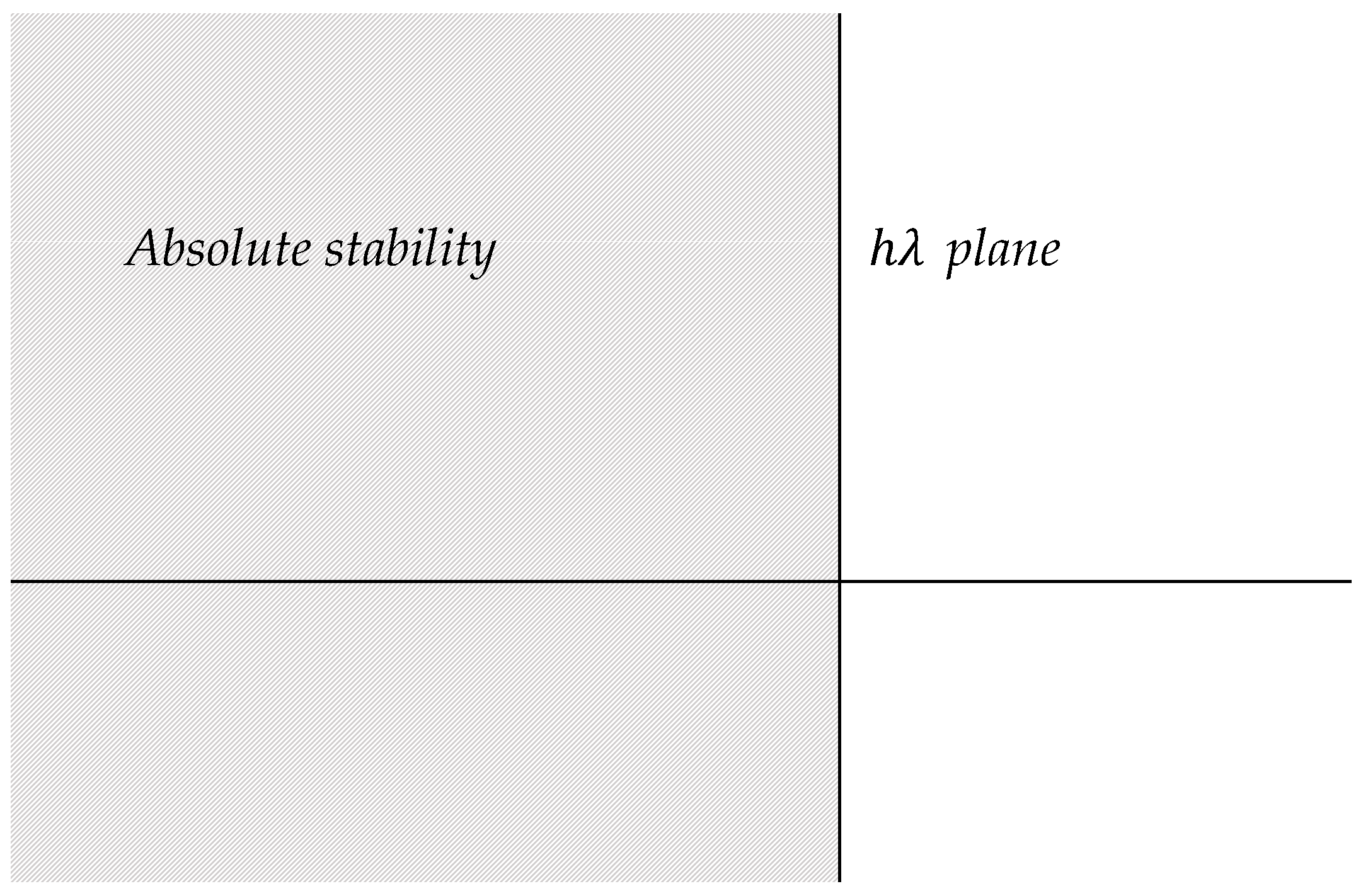
Figure 1. The region of absolute stability for an A-stable method.
Symmetry 11 00846 g001
Figure 2. A ( α ) and stiff stability as presented in [19].
Symmetry 11 00846 g002
Figure 3. The region of absolute stability for A ( α ) -BBDF method.
Symmetry 11 00846 g003
Figure 4. Efficiency curves when solving Problem 1.
Symmetry 11 00846 g004
Figure 5. Efficiency curves when solving Problem 2.
Symmetry 11 00846 g005
Figure 6. Efficiency curves when solving Problem 3.
Symmetry 11 00846 g006
Table 1. Coefficients of the A ( α ) -BBDF.
α 0 , i α 1 , i α 2 , i α 3 , i α 4 , i α 5 , i β i
i = 1 y n + 1 1 / 116 9 / 58 31 / 29 1 27 / 116 1 / 58 24 / 29
i = 2 y n + 2 1 / 73 11 / 146 6 / 73 82 / 73 1 15 / 146 48 / 73
i = 3 y n + 3 15 / 236 23 / 59 1 78 / 59 389 / 236 1 24 / 59
Table 2. Numerical comparison for Problem 1 for the   A ( α ) -BBDF method.
h . MethodNSMAXETIME
10 2 BBDF(5)501.22077 ( 02)3.38123 × 10⁻⁵
3SBBDF341.25970 ( 02)7.97504 × 10⁻⁶
A ( α ) -BBDF349.80872 ( 03)5.74054 × 10⁻⁶
10 4 BBDF(5)5,0003.61596 ( 06)1.95107 × 10⁻⁴
3SBBDF33342.78963 ( 06)2.43208 × 10⁻⁵
A ( α ) -BBDF33342.10240 ( 06)1.81288 × 10⁻⁵
10 6 BBDF(5)500,0003.65378 ( 10)1.19412 × 10⁻²
3SBBDF333,3342.84503 ( 10)2.40965 × 10⁻³
A ( α ) -BBDF333,3342.15115 ( 10)1.24343 × 10⁻³
Table 3. Numerical comparison for Problem 2 for the A ( α ) -BBDF method.
h . MethodsNSMAXETIME
10 2 BBDF(5)2508.22989 ( 05)3.13736 × 10⁻⁵
3SBBDF1676.27205 ( 05)1.42650 × 10⁻⁵
A ( α ) -BBDF1674.80218 ( 05)5.55058 × 10⁻⁶
10 4 BBDF(5)25,0009.13120 ( 09)6.23244 × 10⁻⁴
3SBBDF16,6677.10257 ( 09)2.84914 × 10⁻⁴
A ( α ) -BBDF16,6675.36673 ( 09)3.00451 × 10⁻⁵
10 6 BBDF(5)2,500,0004.75320 ( 11)8.99541 × 10⁻²
3SBBDF1,666,6673.20597 ( 11)1.71905 × 10⁻²
A ( α ) -BBDF1,666,6672.04591 ( 11)3.01268 × 10⁻³
Table 4. Numerical comparison for Problem 3 for the A ( α ) -BBDF method.
h . MethodsNSMAXETIME
10 2 BBDF(5)508.31685 ( 02)4.61774 × 10⁻⁵
3SBBDF341.60854 ( 01)2.57089 × 10⁻⁵
A ( α ) -BBDF341.46790 ( 01)1.13065 × 10⁻⁵
10 4 BBDF(5)50008.63685 ( 05)7.02594 × 10⁻⁴
3SBBDF33346.71328 ( 05)2.17249 × 10⁻⁴
A ( α ) -BBDF33345.06905 ( 05)1.56282 × 10⁻⁴
10 6 BBDF(5)500,0008.64038 ( 09)1.33371 × 10⁻²
3SBBDF333,3346.72941 ( 09)1.62222 × 10⁻²
A ( α ) -BBDF333,3345.08898 ( 09)1.07846 × 10⁻²