Abstract
In this manuscript, by using the weight-function technique, a new class of iterative methods for solving nonlinear problems is constructed, which includes many known schemes that can be obtained by choosing different weight functions. This weight function, depending on two different evaluations of the derivative, is the unique difference between the two steps of each method, which is unusual. As it is proven that all the members of the class are optimal methods in the sense of Kung-Traub’s conjecture, the dynamical analysis is a good tool to determine the best elements of the family in terms of stability. Therefore, the dynamical behavior of this class on quadratic polynomials is studied in this work. We analyze the stability of the presented family from the multipliers of the fixed points and critical points, along with their associated parameter planes. In addition, this study enables us to select the members of the class with good stability properties.
1. Introduction
There is a large number of problems in Science and Engineering modeled by nonlinear equations , where is a vectorial real function defined in a convex set D, with . Usually these problems cannot be analytically solved, so we use iterative schemes. The best known is Newton’s method, the characteristics of which have been improved in much of the research (see, for instance, the texts [1,2] and the references therein). Different techniques have been employed to design these new methods being, in the majority of cases, multistep schemes, due to the limitations of one-step methods.
However, in many applications in geometric modeling, it is necessary to find all the roots of a nonlinear problem within a domain. In these cases, subdivision solvers are the most usual approach when looking for roots globally (see, for example [3] and the references therein). As subdivision solvers usually employ Newton’s scheme when the initial estimation is close to the root, higher order methods as the proposed in this manuscript may be useful to improve the local behavior of these solvers.
The weight function procedure is used to achieve this goal, which is able to increase the order of convergence of known methods (see [1]), achieving optimal schemes under the point of view of Kung-Traub’s conjecture [4]. This conjecture claims that an iterative method without memory which uses d functional evaluations per iteration can reach, at most, order of convergence , being optimal in this bound. Although the aim of many researches in this area is to design optimal high-order methods, it is also known that the higher the order is, the more sensitive the scheme to initial estimations will be.
In our study, through weight function procedure and Newton’s scheme, a new family of iterative methods is presented, with the following iterative expression:
where is a real parameter and the variable of the weight function is .
In the next section, we present the convergence result of this family, describing the conditions that function must satisfy for reaching order four. We also analyze how to extend this structure (1) for designing derivative-free methods and for solving nonlinear systems, . Many known methods, for equations or systems, are particular cases of our class. In Section 3, we study the dynamical behavior of a sub-class obtained by using a particular weight function. The aim of this section is to check how, using complex dynamics tools, we can determine which elements of a given family have good stability properties and which have chaotic behavior.
2. Convergence and Stability
The order of convergence of family (1) is analyzed in the next result, for .
Theorem 1.
Let be a sufficiently differentiable function in an open interval D and let be a simple solution of the nonlinear equation . Starting from a known initial estimation close enough to , if and function H satisfies , , and , then sequence obtained from (1) converges to with order of convergence four, being the error equation
where , and .
Proof.
It is known that and can be expressed as
and
By direct division,
Then,
Again, by expanding in Taylor series,
Therefore,
and, taking into account that t tends to 1 when n tends to infinity, the weight function can be expressed as
where , , and denotes , , and , respectively. Finally,
Therefore, in order to eliminate first order error,
For the second order error:
being
With these values of and , the error equation is now
So, we can eliminate the third order error if
which means that
Hence it is proven that if and function H satisfies , and , the order of convergence is four. □
If we want to design a derivative-free scheme with a similar structure as (1), we change by the divided difference , where with a real parameter, obtaining the following iterative expression:
being in this case the variable of the weight function. Unfortunately, family (2) does not reach order four. However, if we use as variable of the weight function , being , the class
reaches order four under certain conditions as we establish in the following result
Theorem 2.
Let be a sufficiently differentiable function in an open interval D and let be a simple solution of the nonlinear equation . Starting from a known initial estimation close enough to , if and function H satisfies , , and , then sequence obtained from (3) converges to with order of convergence four, being the error equation
where , , and .
On the other hand, family (1) can be extended to the multidimensional case, , so we accomplish a family of iterative methods for solving nonlinear systems , where . In this case, the iterative expression is
where is the Jacobian matrix of F evaluated in the iteration . The variable of weight is and is a matrix function , where , such that
- (i)
- , being the first derivative of H, , and denotes the space of linear mappings from X to itself.
- (ii)
- , being the second derivative of H, and .
- (iii)
- , being the third derivative of H, and .
Then, the Taylor expansion of H around the identity matrix I gives
A similar result to Theorem 1 can be established for class (4), obtaining conditions for function to reach order four. In the proof we use some tools and notations introduced in [5].
Theorem 3.
Let be a sufficiently differentiable function in an convex set D and let be a solution of the nonlinear system , such that is nonsingular. Starting from a known initial estimation close enough to , if and function H satisfies , , and , then sequence obtained from (4) converges to with order of convergence four, being the error equation
where , and .
Proof.
By using Taylor expansion of and around ,
From the above expression, we conjecture
and, from , we have
Then,
Similarly, we calculate
So,
Therefore, variable t of the weight function is described as
and
Therefore,
In order to reach order four, the coefficients of , and must be zero, so
With these values, the error equation is
and the proof is finished. □
Many known schemes designed for solving nonlinear equations or nonlinear systems can be obtained as particular cases of (4) by using different weight functions satisfying the conditions of Theorem 3. For example, the classical Jarratt’s scheme [6]
is obtained from (1) for equations and (4) for systems, by using
In a similar way, the method constructed by Khattri and Abbasbandy in [7] is an element of (4), , by using the weight function
The parametric family of iterative methods for solving nonlinear equations or systems, designed by Kanwar et al. in [8], is a particular case of (1) or (4) using the weight function
where and are free real parameters such that and .
Sharma and Arora published in [9] a method for solving nonlinear systems which we can obtain from (4) by using
Hueso et al. presented in [10] a parametric family of iterative schemes, which is obtained from the weight function
where is a real free parameter.
Finally, Ghorbanzadeh and Soleymani presented in [11] an iterative method solving nonlinear equations or nonlinear systems, which is a particular case of our scheme using the weight function
One of the most simple sub-classes of family (1) is obtained when is the Taylor polynomial of third degree, satisfying , , and , that is, the weight function is:
being the free parameter. In this way, we obtain a parametric family of iterative methods of order four, denoted by CGT. In the next sections, we are going to analyze de dynamical behavior of this class in terms of parameter , for finding the methods with good stability properties and to avoid the elements of the family with chaotic behavior.
3. Stability of Family Cgt
We are going to introduce some concepts of complex dynamics that we need to analyze the stability of the proposed family on quadratic polynomials. These are the most simple nonlinear functions and, although the stability conclusions for quadratic polynomials can not be extended to any nonlinear function, in practice a bad method for quadratic polynomials does not perform adequately for other functions. Moreover, cubic polynomials and high-order iterative methods usually yields to rational operators of very high degree; this makes the analysis unaffordable in the most of cases.
After that, we will calculate the fixed and critical points of the rational operator associated with the class on polynomials. The stability of the fixed points, the behavior of the critical points as initial estimation of the iterative schemes and the basins of attraction of the periodic points give us relevant information about the stability of the methods.
3.1. Basic Concepts On Dynamics
A more complete description of the following concepts can be found in [12]). Given a rational function , where is the Riemann sphere, the orbit of a point is defined as:
We analyze the phase plane of operator R by classifying the starting points from the asymptotic behavior of their orbits.
A is called a fixed point if . A periodic point of period is a point such that and , for . A pre-periodic point is a point that is not periodic but there exists a such that is periodic. A critical point is a point where the derivative of the rational function vanishes, . Moreover, a fixed point is called attractor if , superattractor if , repulsor if and parabolic if .
The basin of attraction of an attractor is defined as:
The immediate basin of attraction of an attractor is the connected component of its basin of attraction that holds the attractor.
The Fatou set of the rational function R, , is the set of points whose orbits tend to an attractor (fixed point, periodic orbit or infinity). Its complement in is the Julia set, . That means that the basin of attraction of any fixed point belongs to the Fatou set and the boundaries of these basins of attraction belong to the Julia set.
The following Theorem establishes a classical result of Fatou and Julia that we use in the study of parameter space associated with the family.
Theorem 4
([13]). Let R be a rational function. The immediate basin of attraction of an attracting fixed or periodic point holds, at least, a critical point.
By using this result, one can be sure to find all the stable behaviors associated with a rational function R, by analyzing the performance of R on the set of critical points.
Taking into account that the proposed family of iterative methods satisfies the Scaling Theorem, it can be seen in the literature ([12]) that the roots of a polynomial can be changed by an affine map without qualitative changes on the dynamics of the family. Therefore, we can use a generic quadratic polynomial .
By replacing by in the iterative expression of the proposed family CGT, the following fixed point operator is obtained:
which depends on parameters , a and b.
In [13], Blanchard considered the conjugacy map , a Möbius transformation with these properties:
It was proven that Newton’s operator, for quadratic polynomials, is conjugate to the rational map . In an similar way, operator on quadratic polynomials is conjugated to operator ,
In this new operator , parameters a and b have been obviated.
3.2. Study of the Fixed Points
Stability and reliability of the members of the family are analyzed in the rest of the paper, regarding the properties of its associate rational function when the class is applied on polynomial . Firstly, fixed points of the rational function are calculated. Specifically, we focus on the points that are not related to the original roots of polynomial , which are named strange fixed points.
In the next result, some properties of the strange fixed points are described.
Theorem 5.
Fixed points of the rational function are the roots of equation . Therefore, we obtain , (corresponding to the roots of ), and the following strange fixed points:
- ,
- the roots of symmetric sixth-degree polynomial , or analogously,
where , and are the roots of the third-degree polynomial , that is,
being .
It is possible to find values of parameter α where two or more strange fixed points coincide. Consequently, operator provides seven strange fixed points, except in the following cases:
- (i)
- If or , there are only five strange fixed points.
- (ii)
- If or the strange fixed points are and the roots of a sixth-degree polynomial, which are two simple and two double roots.
3.3. Stability of the Fixed Points
In this section, we observe that not only the number but also the stability of the fixed points depend on the parameter of the family. This fact can lead to the existence of attracting strange fixed points, which can make the iterative scheme converge to a false solution.
It is known that and are always superattracting fixed points, as the order of convergence of the class is greater than 2. However, relevant numerical information is provided by the stability of the other fixed points (for example, corresponds to the divergence of the original method). Therefore, we determine this stability in the next results.
Theorem 6.
Strange fixed point , with , has the following character:
- (i)
- When , is a repulsor.
- (ii)
- If , is a parabolic point.
- (iii)
- When , then is an attractor.
Proof.
It is easy to prove that
So,
Let us consider an arbitrary complex number. Then,
By simplifying
that is,
Therefore,
□
Stability regions of every strange fixed point (, ) are shown in Figure 1.
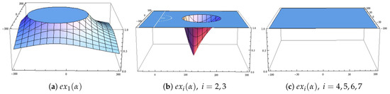
Figure 1.
3D-view of stability functions of strange fixed points.
We can observe from the stability of that these strange fixed points are repulsive for any value of parameter .
3.4. Analysis of the Critical Points
Regarding the dynamics of the family, it is significant to analyze the critical points of the rational function different from 0 and ∞, which are called free critical points.
With the purpose of calculating the critical points, we study which points make null the derivative of .
We know that and , which are related to the roots of the polynomial by means of Möbius map, are critical points and give rise to their respective Fatou components. Nevertheless, several free critical points can be obtained, some of them depending on the value of the parameter .
Proposition 1.
The number of critical points of the rational function depend on the value of the parameter α:
- (a)
- If , there exist one only free critical point, , which is a pre-image of the fixed point .
- (b)
- In all other cases, the free critical points are ,which means that there exists only one independent free critical point.
Proof.
We obtain the previous critical points, since
□
In the case of strange fixed point , we can see that there exist a ball in which the strange fixed points are attractors, whereas outside this ball, are repulsive.
3.5. The Parameter Plane
We have observed that the dynamical behavior of operator depends on the values of the parameter . Taking into account Theorem 4, we are interested in knowing what happens with the free critical points, and if any of them gives rise to a basin of attraction different from those of zero and infinity. In order to have knowledge of this, we obtain the parameter plane associated with the family.
We depict the parameter space associated with a free critical point of operator (6) by associating each point of the parameter plane with a complex value of , i.e., with an element of family (1). Every value of belonging to the same connected component of the parameter space gives rise to subsets of schemes of family (1) with similar dynamical behavior. Therefore, our objective is to find regions of the parameter plane as much stable as possible, due to the fact that the values of in these regions will provide the best members of the family in terms of numerical stability.
Since , we have at most one free independent critical point, consequently, there exist only one parameter plane of the family. If we consider the independent free critical point as a starting point of the iterative schemes of the family associated with each complex value of , this point of the complex plane is painted in red if the method converges to any of the roots (zero and infinity) and they are black in other cases. The lower the number of iterations, the brighter the color used. Following this procedure, we obtain the parameter plane presented in Figure 2, by using the processes described in [14]. We have used a mesh of points, 500 maximum iterations and as the tolerance used in the stopping criterium. We also show a zoom of this parameter plane in Figure 3a, focusing on the biggest red area, where the members of family (1) are, in general, very stable. These would be the best values, a priori, to apply the iterative methods in terms of stability.
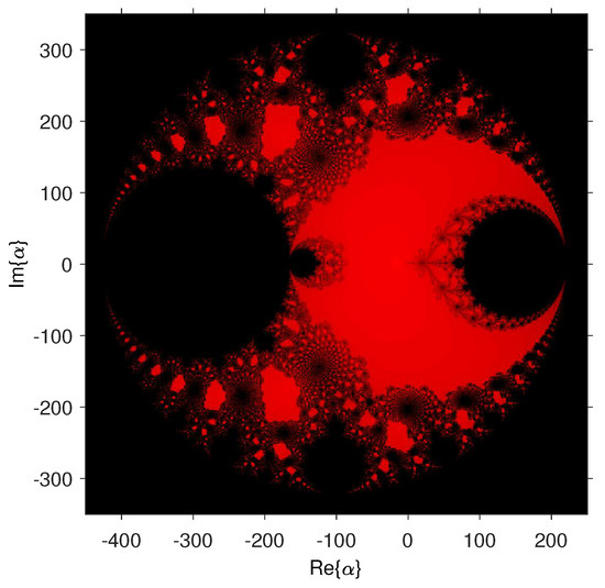
Figure 2.
Parameter plane associated with , .
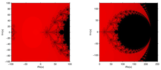
Figure 3.
Details of the parameter plane.
Nevertheless, we can see black regions that inform us about different pathological behavior of the elements of the family. The black ball represented in Figure 3b, correspond to values of parameter for which are attracting. Besides, the big black ball that surrounds the parameter plane in Figure 2 correspond to values of the parameter for which is attracting.
In addition, we can analyze the remaining black regions by drawing dynamical planes with the parameter corresponding to values inside these black regions.
4. Dynamical Planes
Now, we will analyze the qualitative behavior of the different elements of family through the dynamical planes. These elements are selected taking into account the conclusions obtained by studying the parameter plane of the family. Dynamical planes with stable behavior are depicted by using points in the red region of the parameter plane, whereas dynamical planes with unstable performance are calculated with points in the black region of the parameter plane of the family.
Every dynamical plane presented here has been generated by using the routines appearing in [14]. The dynamical plane related to a value of parameter is obtained by iterating an element of family (1). Each point of the complex plane is used as initial estimation. The points whose orbit converges to infinity are plotted in blue, in orange those points converging to zero, in green the points whose orbit converges to one of the strange fixed points, which appear marked as a white star in the figures if they are attracting fixed points, and in black if it reaches the maximum number of 50 iterations without converging to any of the fixed points. A mesh of points has been used and a tolerance of .
Some dynamical planes are shown in Figure 4. These planes correspond to values of the parameter which from the parameter plane, give us elements of the family with stable behavior. Therefore, we can see only two basins of attraction, that correspond to zero (orange basin) and infinity (blue basin).
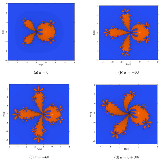
Figure 4.
Some dynamical planes with stable behavior.
On the other hand, as it has been said, unstable behavior is found when we choose values of the parameter in the black region of parameter plane. These dynamical planes are shown in Figure 5.

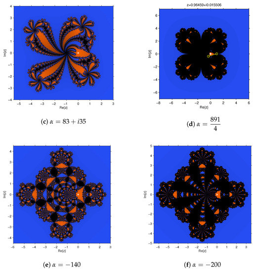
Figure 5.
Some dynamical planes with unstable behavior.
In Figure 5a,c,e,f the dynamical planes of the iterative method corresponding to , , and , respectively, are presented, with regions of slow convergence. Figure 5b, corresponding to , shows the existence of four different basins of attraction, two of them of the superattractors 0 and ∞ and the other ones corresponding to strange fixed points.
Finally, in Figure 5d, corresponding to , we can observe an orbit of period two.
5. Conclusions
In this paper, a class of optimal iterative methods for solving nonlinear equations is presented, which holds many known methods as particular elements. This family is extended in two different directions: a class of derivative-free methods for solving nonlinear equations and a multidimensional family for nonlinear systems. Both classes preserve the order of convergence of the initial family. The dynamical analysis in these areas will be object of study in future works.
Moreover, a complex dynamical study for a parametric sub-family on quadratic polynomials has been presented. We have been able to prove, by means of the parameter plane, that there are many values of with good stability properties, which means that there exist plenty of elements of the family with stable behavior. Nevertheless, there are other values of with convergence anomalies that must be avoided in practical applications.
Author Contributions
The contribution of the authors to this manuscript can be defied as: Conceptualization, A.C. and J.R.T.; Validation, L.G.; Formal Analysis, J.R.T.; Investigation, L.G.; Writing—Original Draft Preparation, A.C.; Writing—Review & Editing, J.R.T.
Funding
This research was partially supported by Spanish Ministerio de Ciencia, Innovación y Universidades PGC2018-095896-B-C22 and Generalitat Valenciana PROMETEO/2016/089.
Acknowledgments
The authors would like to thank the anonymous reviewers that have highly improved the final version of this manuscript.
Conflicts of Interest
The authors declare no potential conflict of interests.
References
- Petković, M.; Neta, B.; Petković, L.D.; Džunić, J. Multipoint Methods for Solving Nonlinear Equations; Academic Press: Amsterdam, The Netherlands, 2013. [Google Scholar]
- Amat, S.; Busquier, S. Advances in Iterative Methods for Nonlinear Equations; Springer SIMAI: Basel, Switzerland, 2016. [Google Scholar]
- Van Sosin, B.; Elber, G. Solving piecewise polynomial constraint systems with decomposition and a subdivision-based solver. Comput.-Aided Des. 2017, 90, 37–47. [Google Scholar] [CrossRef]
- Kung, H.T.; Traub, J.F. Optimal order of one-point and multipoint iteration. J. Assoc. Comput. Math. 1974, 21, 634–651. [Google Scholar] [CrossRef]
- Cordero, A.; Hueso, J.L.; Martínez Torregrosa, J.R. A modified Newton-Jarratt’s composition. Numer. Algor. 2010, 55, 87–99. [Google Scholar] [CrossRef]
- Jarratt, P. Some fourth order multipoint iterative methods for solving equations. Math. Comput. 1966, 20, 434–437. [Google Scholar] [CrossRef]
- Khattri, S.K.; Abbasbandy, S. Optimal fourth order family of iterative methods. Mat. Vesnik 2011, 63, 67–72. [Google Scholar]
- Kanwar, V.; Kumar, S.; Behl, R. Several new families of Jarratt’s method for solving systems of nonlinear equations. Appl. Appl. Math. 2013, 8, 701–716. [Google Scholar]
- Sharma, J.R.; Arora, H. Efficient Jarratt-like methods for solving systems of nonlinear equations. Calcolo 2014, 51, 193–210. [Google Scholar] [CrossRef]
- Hueso, J.L.; Martínez, E.; Teruel, C. Convergence, efficiency and dynamics of new fourth and sixth order families of iterative methods for nonlinear systems. Comput. Appl. Math. 2015, 275, 412–420. [Google Scholar] [CrossRef]
- Ghorbanzadeh, M.; Soleymani, F. A Quartically convergent Jarratt-type method for solving systems of equations. Algorithms 2015, 8, 415–423. [Google Scholar] [CrossRef]
- Blanchard, P. Complex Analytic Dynamics on the Riemann Sphere. Bull. AMS 1984, 11, 85–141. [Google Scholar] [CrossRef]
- Blanchard, P. The Dynamics of Newton’s Method. Proc. Symp. Appl. Math. 1994, 49, 139–154. [Google Scholar]
- Chicharro, F.; Cordero, A.; Torregrosa, J.R. Drawing dynamical and parameter planes of iterative families and methods. Sci. World J. 2013, 2013, 780153. [Google Scholar] [CrossRef] [PubMed]
© 2019 by the authors. Licensee MDPI, Basel, Switzerland. This article is an open access article distributed under the terms and conditions of the Creative Commons Attribution (CC BY) license (http://creativecommons.org/licenses/by/4.0/).