Abstract
Automatic gender classification is challenging due to large variations of face images, particularly in the un-constrained scenarios. In this paper, we propose a framework which first segments a face image into face parts, and then performs automatic gender classification. We trained a Conditional Random Fields (CRFs) based segmentation model through manually labeled face images. The CRFs based model is used to segment a face image into six different classes—mouth, hair, eyes, nose, skin, and back. The probabilistic classification strategy (PCS) is used, and probability maps are created for all six classes. We use the probability maps as gender descriptors and trained a Random Decision Forest (RDF) classifier, which classifies the face images as either male or female. The performance of the proposed framework is assessed on four publicly available datasets, namely Adience, LFW, FERET, and FEI, with results outperforming state-of-the-art (SOA).
1. Introduction
Automatic gender classification is a fundamental task in computer vision, which has recently attracted immense attention. It plays an essential role in a wide range of real-world applications such as targeted advertisement, forensic science, visual surveillance, content-based searching, human-computer interaction systems, etc. However, gender classification is still an arduous task due to various changes in visual angles, face expressions, pose, age, background, and face image appearance. It is more challenging in the un-constrained imaging conditions.
Automatic gender classification is already addressed in computer vision. The literature reported many useful algorithms for gender classification; however, geometric modeling methods are most commonly used. In geometric modeling, face parts are located through prior facial landmarks localization models [1,2,3,4], and then gender classification is performed. The performance of gender classification in such cases highly depends on the most accurate localization of these face parts. The face landmarks localization is itself a big challenge. The performance of points localization models is significantly affected in cases such as background, occlusion, face image rotation, and if the face images are of poor quality. Similarly, these landmarks localization is extremely difficult in far-field imagery conditions. As landmarks, localization models are facing severe problems, and we approached the gender classification task in an entirely different way.
Previous literature reported that gender classification was addressed as an individual research problem through a different set of techniques [5,6,7,8,9]. We argue all face analysis tasks are closely related and can help each other if sufficient information about face parts is provided. This fact is also confirmed by the psychophysical studies stating that: “key face features (such as nose, mouth, and eyes) help human visual processing systems to categorize face images [10,11]”. We already tackled the multi-class face segmentation task in our previous work (MSFS) [12], and successfully applied MSFS [12] to the head pose estimation (MSFS-HPE) [13]. Our current research work is part of a long term-research strategy leading to a single unified framework for face image analysis.
As far as we know, previously face segmentation was considered as a three or four classes segmentation task. In the MSFS [12], we extended the face segmentation to six classes, i.e., hair, nose, mouth, eyes, skin, and back. However, we were facing two significant problems with MSFS [12]. Firstly, the testing phase of the MSFS [12] was taking a long time, as a class label was provided to each pixel in a face image. To reduce the computational cost of the segmentation part, we replaced the pixel-based approach with a super-pixel. Secondly, the MSFS [12] was not considering any conditional hierarchy between face parts. For example, it is very unlikely for the mouth region near the eye and vice versa. In this paper, we introduced the CRFs based modeling method, which considers all labels in a face image in a proper hierarchy. The MSFS-CRFs improved the average pixel labeling accuracy (PLA) of the segmentation part from 92.4% to 96.7%.
A summary of the main contributions of this paper is:
- We introduce a new face segmentation algorithm called MSFS-CRFs. The MSFS-CRFs is an extension of our previous work, MSFS [12]. The new algorithm couples the labeling information between six different face parts.
- We propose a new automatic gender classification algorithm, called GC-MSFS-CRFs. We use the PCS and generated probability maps for all classes. The probability maps are used as gender descriptors, and an automatic gender classification algorithm is developed.
- We evaluate the two new models ( MSFS-CRFs and GC-MSFS-CRFs) on four face databases, and better and competitive results are reported.
The structure of the remaining paper is as follows: Section 2 presents related work for gender classification. The proposed gender classification method is presented in Section 3. We summarized the obtained results and also discussed important points in Section 4. The conclusions and future directions are presented in Section 5.
2. Background and Related Work
A rich amount of literature already exists on the topic of gender classification. It is not possible to organize all previous methods into a single ubiquitous taxonomy in the current paper; however, we provided a quick overview of how researchers previously approached gender classification.
The earlier methods which addressed the gender classification problem are known as appearance-based methods. In the appearance based methods, features are extracted from face images—considering face as a one-dimensional feature vector and then a classification tool is used. Some earlier researchers extracted pixel intensity values as well and then fed these values to the classifiers (for instance, see [14]). The pre-processing steps included face alignment, image re-sizing, and illumination normalization. The sub-space transformation was also performed either to reduce dimensions or explore parts of the underlying structure of the image raw data [15]. Typically, the classification is performed through a binary classification strategy. The mostly used classifier for the automatic gender classification is a support vector machine; other classifiers applied included decision trees, neural networks, and AdaBoost [14,16,17,18,19]. For more detailed information about gender classification methods, a review paper in [15] can be explored.
Recently, a new gender classification algorithm is proposed in [20]. Authors of the paper performed tests on two databases FEI [21] and a self-built database. Different kinds of texture features were extracted from face images. The texture features were extracted from three discriminating levels, including global, directional, and regional. A kernel-based support vector machine was used later on for the classification stage.
The other methods which are used for gender classification are known as geometric methods. These models extract facial landmark information from face images and build a model based on landmarks information. The geometric models maintain a certain geometric relationship between different face parts. These models discard facial texture information in the whole modeling process. As discussed in Section 1, these models are highly sensitive to imaging geometry and face alignment. Some methods that used the idea of geometric modeling are presented in [1,2,3,4,22,23,24].
Several hybrid models for gender and other face attributes are also reported in the literature. A combined framework for gender and age was introduced in [25]. According to the authors of the paper, it was a viewpoint invariant model showing robustness to scale rotation at the local level. A new dataset for gender and age classification was also proposed in [26]. Authors of the paper suggested a hybrid pip-line for gender and age study. Similarly, a semantic pyramid for gender and action recognition was designed in [27]. Another paper [28] proposed a mechanism that combined the name of first part of the information with face images and performed gender classification. A complete face analysis algorithm is proposed in [29], which tackled the three face analysis tasks (gender, race, and age) in a single framework.
Deep Convolutional Neural Networks (CNNs) showed outstanding performance for various image recognition problems. The CNN based methods are applied to both feature extraction as well as classification algorithm for the automatic gender classification [30]. A hybrid system for gender and age classification was presented in [31]. Features were extracted through CNNs, and an extreme learning machine (ELM) was used for classification. This hybrid model is known as ELM-CNNs in the literature. The ELM-CNNs were evaluated on two public databases, MORPH-II [32] and Adience [26]. The ELM-CNN is the best algorithm performing on gender classification thus far.
All of the methods mentioned above contributed a lot to the gender classification problem. However, most of these algorithms were evaluated on the data sets which were collected in very constrained imaging conditions. We validated our framework on four publicly available face databases, namely Adience [26], LFW [33], FEI [21], and FERET [34]. Two of the four databases (Adience and FLW) were collected in the real-world un-constrained conditions. The obtained results are very interesting and encouraging, confirming the effectiveness of the proposed framework for the gender classification task.
3. Proposed Methods
We present our main contributions in this section. The Section 3.1 presents the face segmentation part, whereas the Section 3.2 is about the gender classification.
3.1. Proposed MSFS-CRFs
Face parts are not localized in most of the publicly available face datasets. We apply a face detection algorithm to each face image. Face detection is a very mature research topic in computer vision. There are many excellent face detection algorithms that have been previously reported. Therefore, instead of using our own, we apply a CNNs based face detector introduced in [35]. After face parts localization, images are re-scaled to a size having height 128 pixels and the width is adjusted in order to keep the original face image ratio.
To estimate various face parts segmentation, we use CRFs [36]. The segmentation probability S is encoded with given features X of a face image. Initially, we segment a face image into super-pixels with the widely used SEEDs algorithm [37]. The X is a combination of both node and edge features, represented by and respectively. Let us represent the segmentation with S, which is S = , where n is the total number of super-pixels in the segmented image.
The node and edge energies are represented with and respectively. The log linear CRFs model developed is (Algorithm 1):
where is the set node weights for each label k, is a set of edge weights for each pair of labels ( ). For edge potential, we keep the setting such that , showing a symmetric edge potential conditions.
The probability of segmentation S given X is represented as:
In Equation (3), the double sum is taken for neighboring super-pixels, and N(X) represents the partition function. The partition function works as a normalization factor for the entire distribution. In the proposed MSFS-CRFs model, we use the Bethe Approximation [38] for the partition function. To achieve marginal approximation, we use loopy belief propagation. To optimize the MSFS-CRFs model, we utilize the algorithm L-BFGS [39]. Lastly, we add the Gaussian model to regulate weights.
| Algorithm 1 Proposed GC-CRFs algorithm |
| Input: training data: I = {(P,Q)}, I. where the model is trained through I and evaluated through I. The symbol P represents the input training image and Q(i,j)∈ {1,2,3,4,5,6} the ground truth manually annotated image. a: Face segmentation model : Step a.1: Training a CRFs based model through training data. Step a.2: Dividing each testing image intro super-pixels and finding the center of each super-pixel. Creating a bounding box/patch around the central pixel and passing the patch to the model Step a.3: Using the PBS and generating probability maps for all six classes, represented as: Pb, Pb, Pb, Pb, Pb, and Pb b. Gender classification part: Creating a feature vector from each face image such that: Pb + Pb + Pb + Pb c. Training an RDF classifier for gender classification Output: Predicted gender |
We apply L1 error to every segmentation estimate to assess the segmentation accuracy. Similarly, we also added the penalty to each super-pixel according to the difference of the accurate label prediction and probability value 1—for example, for a super-pixel having a probability of 0.8 for being mouth class, whereas mouth is also the ground truth label, we added a penalty of value 0.2.
From node features, we extract three types of information from face images, including position, color, and shape.
For position features, we consider a 16×16 grid and then the relative location of the central pixel is located. We define this location as:
where the patch width and height are represented with W and H, respectively.
The literature reports the best results for color information with an HSV (hue, saturation, and variance) histogram. We concatenate the three values—hue, saturation, and variance—to form a single vector for color information. We keep the dimension of patch for HSV as = 16 × 16. We set the number of binaries 32 during experiments. Fixing all the values, we create a feature vector for color as .
We use HOG (histogram of oriented gradient) [40] for shape information. For HOG features, we keep the patch size as = 64 × 64, resulting in a feature vector of .
We concatenate all three of the features to form a single unique feature vector represented as .
3.2. Proposed GC-MSFS-CRFs
We summarize the proposed Algorithm 1. We build a CRFs based segmentation model as an initial step. The CRFs based model segments a face image into the most likely class for each super-pixel. Each super-pixel consists of several pixels that attain the same class label from the trained model. We use PCS and created probability maps for each class in a face image. We represent these probability maps as Pb, Pb, Pb, Pb, Pb, and Pb. Some images from the FEI dataset and its segmentation results with probability maps are shown in Figure 1.
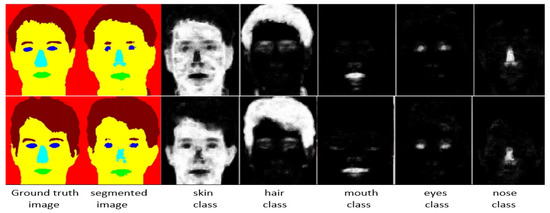
Figure 1.
Images segmented with the proposed MSFS-CRFs along with probability maps for all face classes. For each column (1–7), the corresponding label is added at the bottom (images are taken from the FEI database).
We use RDF to train the model, exploiting the C++ ALGLIB [41] implementation. In our algorithm implementation, we also need probability values for all the six classes along with class label, for which ALGLIB is the best choice. The ALGLIB is a cross-platform numerical analysis library that is a modification of the original Random Forest algorithm designed by Leo Breiman and Adele Cutler [42].
The RDF implementation of ALGLIB needs three parameters to be adjusted. Firstly, the ratio r, which is the size of the part of the training set used for the construction of an individual tree. After a large number of experiments, we set this value 0.95. Secondly, the number of trees denoted as NTree are set as 90. Lastly, the NClasses showing the number of classes used is set 6.
The advantages of the library are high training speed, non-iterative training, scalability, and a small number of parameters to be adjusted. The disadvantages are a large memory capacity needed for building the model; the developed model works slower and is prone to overfitting.
We used the generated probability maps as feature descriptors and trained an RDF classifier through it. To know which probability maps help in gender recognition, we conducted a broad set of experiments. We also did a detailed study from computer vision and human anatomy literature to know which face parts give a gender feminine or masculine characteristics. In the following paragraphs, we summarize this information.
- Face anatomy literature reports that the male forehead is larger compared to the female. In some cases, the hairline is entirely missing in males, for example, if the subject has baldness. This results in a larger forehead in males compared to females. Consequently, our MSFS-CRFs generates a brighter probability map for the class skin in males, extended to most of the face images. Figure 2 and Figure 3 show probability maps for female and male subjects, respectively, for all four classes (skin, hair, eyes, and nose).
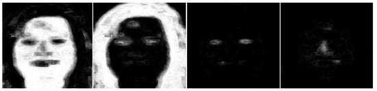 Figure 2. Probability maps’ images of a single female subject for four semantic classes, namely, skin, hair, eyes, and nose (images are taken from the FEI database).
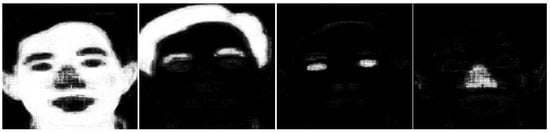 Figure 3. Probability maps’ images of a single male subject for four semantic classes, namely, skin, hair, eyes, and nose (images are taken from FEI database).
 - It can be observed from face images that females have larger eyelashes, which are curly. Our CRFs based segmentation model classifies these eyelashes with hair. Due to this incorrect classification, the PLA for eyes is lower in females compared to males (females: 82% and males: 86%). However, this misclassification helps the gender recognition problem, as brighter probability maps are generated for males in larger areas compared to females. Please see Figure 2 and Figure 3 for comparison.
- Generally, the male nose is comparatively larger. Similarly, the bridge and ridge of the male nose are also more significant. The literature reports that the male body is larger compared to the female. This larger body has bigger lungs which need sufficient passages for air supply towards the lungs. All of this results in larger nostrils in males compared to females.
- Hairstyle has very complex geometry, which varies from person to person. Our MSFS-CRFs model extracts this geometry very efficiently. We achieve PLA of 96.65% for the hair class, the second highest PLA value in all classes. From Figure 1, it can be observed that our segmentation model extracts this hairline efficiently. We encode this information as a feature descriptor and use it in our gender classification algorithm.
- While creating ground truth data, we use the same label for eyebrows and hair. These eyebrows also help in gender recognition. Female eyebrows are longer, thinner, and curly at the ends. On the other hand, male eyebrows are mismanaged and thicker. The segmentation part extracts this information from face images, which further help in gender classification.
- From previous literature, we observe that the mouth must help in gender classification. As females use different kinds of makeup, generally, their lips are brighter and more visible. On the other hand, male lips are not that very bright. In some images in males, the upper lip is missing in some cases. We achieve a PLA of 77.23% for mouth class. As per the literature and our reported PLA value (77.23%), mouth class must help to improve the classification rate for gender recognition. However, we observe no improvement while using mouth class. On the other hand, with the inclusion of mouth class in the GC-MSFS-CRFs, the computational cost was increased. Therefore, we do not consider mouth information in our GC-MSFS-CRFs model.
We manually labeled 50 images from each database and each gender to train a CRFs based segmentation model. The probability maps for four classes are used as feature descriptors and concatenated with each other to form a single feature vector. The feature vector created is used to train and test the proposed gender classification algorithm. The probability maps for four classes for female and male images are shown in Figure 2 and Figure 3, each of which is used as gender feature descriptors.
4. Experiments and Results
4.1. Used Databases
We used four face databases to evaluate our proposed work, namely Adience [26], LFW [33], FEI [21] and FERET [34].
- Adience Benchmark: It is a new database which was released in 2017. The database was collected in the un-constrained conditions and was used for gender and age classification. The images in the Adience database were obtained through smartphone devices. Different variations, such as lighting, facial appearance, nose, and pose, were included to make the database more challenging. The total number of face images in the Adience was 26,580, with 2284 participants. The dataset is available from the computer vision lab of the University of Israel.
- LFW database: The LFW database was also collected in wild conditions. The total face images in the LFW were 13,233, with 5479 participants. All of the face images were collected from the internet; consequently, the quality of the images is very poor, as most of the images are in the compressed form. Face parts in the images were localized through the Viola-Jones face detector [33]. It is a highly imbalanced database as the number of male subjects are 10,256, whereas female subjects total 2977.
- FERET database: It is an old database which was previously used as a benchmark for different facial recognition algorithms. All images were collected in indoor lab conditions; therefore, the database is comparatively simple. The total number of face images was 14,126, with 1199 participants. To bring a bit of complexity to the images, facial expression, lighting conditions, and face poses were changed slightly. In the proposed work, we used the colored version of the database. The dataset consisted of both frontal and profile face images. We considered both frontal and profile images in our experiments.
- The FEI database: The FEI is a Brazilian dataset which contained images of 200 individuals. Each subject had 14 images, and the total number of images in the database was 2800. All of the images were colored with a flat white background. The age of all the subjects was in the range of 19–40 years. Some changes in the face appearance such as hairstyle and adornments were also added. It is a very balanced database as far as gender classification task is concerned, as half of the subjects are male and half female.
4.2. Experimental Setup
For face segmentation, we used only the FEI database. The FEI database consists of 2400 images. We randomly selected 100 images and manually labeled these images. Hence, the training set contains just 100 images, and the remaining 2300 images were used for the testing phase. The reported results for face segmentation are for the FEI database only.
For gender classification, we randomly manually labeled 100 images from each of the four databases. We trained an MSFS-CRFs model through those 100 images for each database. We performed gender classification tests on the remaining set of images for every four databases. The MSFS-CRFs creates probability maps for all six classes and all testing images. After creating probability maps for all testing phase images, we performed 10-fold cross-validation experiments. We used 90% data for training an RDF model and 10% for testing. We repeated this setting ten times and the average results are reported in the paper.
There is no repletion of training set data in the testing set during our gender classification experiments. The 10-fold validation protocol is usually used to estimate how a built model is expected to perform in general when used to make predictions on data not seen during the training phase of the model. Importantly, each observation in the data sample is assigned to an individual group and stays in that group for the duration of the procedure. This means that each sample is allowed to be used in the hold out set one time and used to train the model for the remaining times.
4.3. Results Discussion
4.3.1. Super-Pixels Parameters Setting
Superpixel algorithms aim to over-segment the face image by grouping pixels that belong to the same object. In the proposed work, we used the hill-climbing optimization algorithm SEEDs, which divides an image into super-pixels based on the object size inside the image. We did not develop our own super-pixel algorithm, but we use SEEDs for super-pixel segmentation.
The size of the super-pixels is not the same throughout the image segmentation. It varies with underlying contents of the image. For example, in the image area, where small changes occur in the nearby pixels, the size of the super-pixels is large (e.g., background). For the remaining face parts, the size of the super-pixel is comparatively small.
For various parameters setting for super-pixels, we performed a large number of experiments. We observed better results with 485 super-pixels. The number of super-pixels highly depend on block levels and image size. When we increased the size and block levels, better segmentation was noticed. Due to computational restrictions, we kept the image size with width of 128 pixels and its corresponding height. We used block level 3 and the histogram bins 6.
4.3.2. Face Segmentation Results
To the best of our knowledge, our previous work [12] for the first time extended face segmentation to six classes. However, we were facing two major issues with MSFS [12]. Firstly, its computational cost was too high, and, secondly, it did not consider any conditional hierarchy between different face parts.
To reduce the computational cost, we replaced the pixel-based method with the super-pixel. In the MSFS [12], a test image is first segmented into super-pixels. Each pixel within the super-pixel attained the same class label as a superpixels label. For super-pixel segmentation, we used SEEDs—as SEEDs has much better speed and excellent segmentation results as reported with standard error metrics [37]. We improved the computational cost five times with our proposed model, i.e., MSFS-CRFs. For example, an image of size 128 × 168 was segmented previously in 50 seconds. The same image segmentation time is reduced to eight seconds in the new framework.
Face segmentation results for frontal images were much better compared to non-frontal, as expected. Some images taken from the FEI database and segmented with MSFS-CRFs are shown in Figure 1. From Figure 1, it is clear that we have better results for bigger classes (skin, hair, and back), and comparatively poor results for smaller classes (nose, eyes, and mouth). This fact is also confirmed by the confusion matrix shown in Figure 1. In the Table 1, we report the PLA values for frontal images only (FEI database).

Table 1.
Frontal images PLA values for images taken from FEI database.
We compared the performance of our proposed segmentation model (MSFS-CRFs) with previously proposed MSFS [12] in Figure 4. From Figure 4, it is clear that we improved PLA values for all the six classes. The most beneficial classes are smaller classes, particularly the nose. The PLA of the nose increased from 29.8% to 75.8%, which is improvement by a large margin.
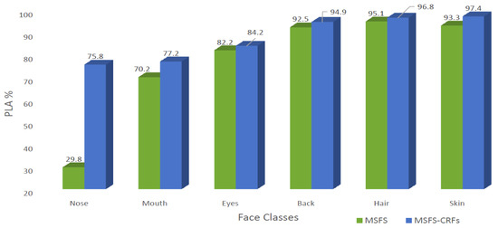
Figure 4.
Performance comparison for PLA of MSFS and MSFS-CRFs models.
4.3.3. Gender Classification
We manually labeled 50 images from each dataset and each gender. We generated the ground truth images through an image editing software. We did not use any automatic segmentation tool during this process. Such type of ground truth data labeling has two drawbacks. Firstly, the manual labeling method is a very tedious and time-consuming task. It is not possible to label hundreds and thousands of images by a single subject through this method. Secondly, this process depends on the subjective perception of only humans involved in the labeling process. It is challenging to provide the exact label to all pixels in a face image, mainly, on the boundary region of the two face parts. For example, drawing a boundary between the nose and skin is very difficult.
We believe it is very difficult to achieve a fair and exact comparison with state-of-the-art (SOA) methods as different authors used different validation protocols and different image settings. In our proposed work, we used 10-fold cross-validation protocol. However, we excluded those 100 images from the testing phase, which were previously used to build an MSFS-CRFs model for each database. All best possible combinations of the six features were tried during experiments. A very detailed overview is already presented in Section 3, with valid reasons why we used four face parts (nose, skin, eyes, and hair). Initially, face parts were localized through a CNNs based [35] face detector. After face detection, images were re-scaled to a constant height 128 and its corresponding width.
We reported our gender recognition results with classification accuracy (C), defined as the correct gender classification to the total number of male and female images processed. We performed our gender classification tests with four datasets. These datasets included Adience, LFW, FEI, and FERET. Summary of the results is presented in Table 2. We also compared our results with SOA in Table 2. From Table 2, it is clear that we have much better results with three datasets as compared to previously reported results.
Table 2.
Comparative experiments on automatic gender classification using the datasets Adience, FEI, LFW and FERET.
We want to clarify a point regarding the reported results in Table 2. From Table 2, it can be seen that, when we used the FEI database, we obtained C of 93.7%, which is less than the other previously proposed methods. All of these methods evaluated their framework on a subset of images, i.e., frontal images. Moreover, the validation protocols were also different (for instance, 2-fold in case [47]), and not clear in the other methods [20,49]. We evaluated GC-MSFS-CRFs on 2700 frontal as well as profile images. It should be noted that the total face images in the FEI are 2800. We randomly selected 100 images for building the MSFS-CRFs model and later on excluded those 100 images from the gender classification testing phase.
In short, to obtain an accurate statistical comparison of GC-MSFS-CRFs with methods as in Table 2, a confidence interval is needed in the performance metric. We need to randomize all the data and run all the algorithms again. This is possible for our method but not for the remaining methods as in Table 2, as we require re-implementing these algorithms from scratch.
We noticed that the performance of the segmentation part depends on the quality of the images. For example, when tests with the LFW were performed, comparatively weak results were noticed. As all images in the LFW were collected from the internet and had very poor resolution, PLA was also dropped. This leads to the comparatively poor performance of the gender recognition part for the LFW database.
We also report results in the form of Precision, Recall, and F-1 Measure. These results are presented in Table 3. For the FERET database, we have perfect results, and hence these are not included in Table 3. Previously reported methods do not provide information for Precision, Recall and F-1 Measure.
Table 3.
Precision, Recall, and F-1 Measure values for all the used datasets through the proposed algorithm GC-MSFS-CRFs.
In most of the cases, we obtained better results compared to SOA, even considering recently introduced CNNs based methods. We are not disparaging CNNs based methods through this comparison—we believe a better understanding of these CNNs based methods and their implementation in different tasks is still needed.
In a nutshell, the performance of the proposed GC-MSFS-CRFs is very interesting and better or competitive results are obtained compared to SOA. We derive an observation from the reported results and experiments: “A correlation exists between various face parts segmentation and its gender. An exact face parts segmentation leads to accurate gender classification and vice versa”.
5. Conclusions
In this paper, we propose a gender classification framework through face parts segmentation. We build a face segmentation model through CRFs. The CRF uses the idea of various face parts hierarchy and their mutual relationship with each other. For training the CRFs based model, three kinds of features are extracted from nodes, namely position, color, and shape information. The CRFs based model segments a face image into six classes, i.e., hair, eyes, nose, mouth, back, and skin. We use PCS and generated probability maps for all six of the classes. The generated probability maps are used as feature descriptors, and an RDF classifier is trained. A set of experiments are conducted to know which face parts help a face image in gender classification.
Our segmentation model provides very useful information for various “natural hidden variables" in a face image. We argue that this information provides a route towards more complicated face analysis problems such as complex facial expression, ethnicity recognition, etc. We also plan to improve the performance of the segmentation part by switching to the newly introduced CNNs based models.
Author Contributions
Conceptualization, K.K. and I.S.; methodology, K.K.; software, M.A.; validation, K.K. and A.G.; formal analysis, A.G.; investigation, M.A.; resources, M.A.; data curation, K.K.; writing—original draft preparation, K.K.; writing—review and editing, K.K., M.A., I.S. and A.G.; visualization, K.K.; supervision, K.K.; project administration, K.K.
Funding
This research received no external funding.
Acknowledgments
We are immensely grateful to the anonymous reviewers and editor for their comments on an earlier version of the manuscript.
Conflicts of Interest
The authors declare no conflict of interest.
References
- Matthias, D.; Juergen, G.; Gabriele, F.; Luc, V.G. Real-time facial feature detection using conditional regression forests. In Proceedings of the 2012 IEEE Conference on Computer Vision and Pattern Recognition, Washington, DC, USA, 16–21 June 2012; pp. 2578–2585. [Google Scholar]
- Rlph, G.; Iain, M.; Simon, B. Generic vs. person specific active appearance models. Image Vis. Comput. 2005, 23, 1080–1093. [Google Scholar]
- Syed, Z.G.; Ajmal, M. Perceptual differences between men and women: A 3D facial morphometric perspective. In Proceedings of the IEEE 22nd International Conference on Pattern Recognition, Stockholm, Sweden, 24–28 August 2014. [Google Scholar]
- Rajeev, R.; Vishal, M.P.; Rama, C. HyperFace: A deep multi-task learning framework for face detection, landmark localization, pose estimation, and gender recognition. IEEE Trans. Pattern. Anal. Mach. Intell. 2019, 41, 121–135. [Google Scholar]
- Ping-Han, L.; Jui-Yu, H.; Yi-Ping, H. Automatic gender recognition using fusion of facial strips. In Proceedings of the 20th International Conference on Pattern Recognition, Istanbul, Turkey, 23–26 August 2010; pp. 1140–1143. [Google Scholar]
- Jordi, M.; Alberto, A.; Roberto, P. Local deep neural networks for gender recognition. Pattern Recognit. Lett. 2016, 70, 80–86. [Google Scholar]
- Juan, B.C.; Jose, M.B.; Luis, B. Robust gender recognition by exploiting facial attributes dependencies. Pattern Recognit. Lett. 2014, 36, 228–234. [Google Scholar]
- Caifeng, S. Learning local binary patterns for gender classification on real-world face images. Pattern Recognit. Lett. 2012, 33, 431–437. [Google Scholar]
- Modesto, C.S.; Javier, L.N.; Enrique, R.B. On using periocular biometric for gender classification in the wild. Pattern Recognit. Lett. 2016, 82, 181–189. [Google Scholar]
- Graham, D.; Hayden, E.; John, S. Perceiving and Remembering Faces; Academic Press: Cambridge, MA, USA, 1981. [Google Scholar]
- Sinha, P.; Balas, B.; Ostrovsky, Y.; Russell, R. Face recognition by humans: Nineteen results all computer vision researchers should know about. Proc. IEEE 2006, 94, 1948–1962. [Google Scholar] [CrossRef]
- Khan, K.; Mauro, M.; Leonardi, R. Multi-class semantic segmentation of faces. In Proceedings of the IEEE International Conference on Image Processing (ICIP), Quebec, QC, Canada, 27–30 September 2015; pp. 827–831. [Google Scholar]
- Khan, K.; Mauro, M.; Migliorati, P.; Leonardi, R. Head pose estimation through multi-class face segmentation. In Proceedings of the 2017 IEEE International Conference on Multimedia and Expo (ICME), Hong Kong, China, 10–14 July 2017; pp. 175–180. [Google Scholar]
- Moghaddam, B.; Yang, M.H. Learning gender with support faces. IEEE Trans. Pattern Anal. Mach. Intell. 2002, 24, 707–711. [Google Scholar] [CrossRef]
- Ng, C.B.; Tay, Y.H.; Goi, B.M. A review of facial gender recognition. Pattern Anal. Appl. 2015, 18, 739–755. [Google Scholar] [CrossRef]
- Makinen, E.; Raisamo, R. Evaluation of gender classification methods with automatically detected and aligned faces. IEEE Trans. Pattern Anal. Mach. Intell. 2008, 30, 541–547. [Google Scholar] [CrossRef]
- Yu, S.; Tan, T.; Huang, K.; Jia, K.; Wu, X. A study on gait-based gender classification. IEEE Trans. Image Process. 2009, 18, 1905–1910. [Google Scholar] [PubMed]
- Golomb, B.A.; Lawrence, D.T.; Sejnowski, T.J. Sexnet: A neural network identifies sex from human faces. Conf. Adv. Neural Inf. Process. Syst. 1990, 3, 572–577. [Google Scholar]
- Baluja, S.; Rowley, H.A. Boosting sex identification performance. Int. J. Comput. Vis. 2006, 71, 111–119. [Google Scholar] [CrossRef]
- Geetha, A.; Sundaram, M.; Vijayakumari, B. Gender classification from face images by mixing the classifier outcome of prime, distinct descriptors. Soft Comput. 2019, 23, 2525–2535. [Google Scholar] [CrossRef]
- Centro Universitario da FEI, FEI Face Database. Available online: http://www.fei.edu.br/~cet/facedatabase.html (accessed on 13 May 2019).
- Ferrario, V.F.; Sforza, C.; Pizzini, G.; Vogel, G.; Miani, A. Sexual dimorphism in the human face assessed by Euclidean distance matrix analysis. J. Anat. 1993, 183, 593. [Google Scholar] [PubMed]
- Burton, A.M.; Bruce, V.; Dench, N. What’s the difference between men and women? Evidence from facial measurement. Perception 1993, 22, 153–176. [Google Scholar] [CrossRef] [PubMed]
- Fellous, J.M. Gender discrimination and prediction on the basis of facial metric information. Vis. Res. 1997, 37, 1961–1973. [Google Scholar] [CrossRef][Green Version]
- Toews, M.; Arbel, T. Detection, localization, and sex classification of faces from arbitrary viewpoints and under occlusion. IEEE Trans. Pattern Anal. Mach. Intell. 2009, 31, 1567–1581. [Google Scholar] [CrossRef] [PubMed]
- Eidinger, E.; Enbar, R.; Hassner, T. Age and gender estimation of unfiltered faces. IEEE Trans. Inf. Forensics Secur. 2014, 9, 2170–2179. [Google Scholar] [CrossRef]
- Khan, F.S.; Van De Weijer, J.; Anwer, R.M.; Felsberg, M.; Gatta, C. Semantic pyramids for gender and action recognition. IEEE Trans. Image Process. 2014, 23, 3633–3645. [Google Scholar] [CrossRef]
- Chen, H.; Gallagher, A.C.; Girod, B. The hidden sides of names—Face modeling with first name attributes. IEEE Trans. Pattern Anal. Mach. Intell. 2014, 36, 1860–1873. [Google Scholar] [CrossRef] [PubMed]
- Han, H.; Otto, C.; Liu, X.; Jain, A.K. Demographic estimation from face images: human vs. machine performance. IEEE Trans. Pattern Anal. Mach. Intell. 2015, 37, 1148–1161. [Google Scholar] [CrossRef] [PubMed]
- Levi, G.; Hassner, T. Age and gender classification using convolutional neural networks. In Proceedings of the IEEE Conference on Computer Vision and Pattern Recognition Workshops, Boston, MA, USA, 7–12 June 2015; pp. 34–42. [Google Scholar]
- Duan, M.; Li, K.; Yang, C.; Li, K. A hybrid deep learning CNN–ELM for age and gender classification. Neurocomputing 2018, 275, 448–461. [Google Scholar] [CrossRef]
- Ricanek, K.; Tesafaye, T. Morph: A longitudinal image database of normal adult age-progression. In Proceedings of the Seventh International Conference on Automatic Face and Gesture Recognition, Southampton, UK, 10–12 April 2006; pp. 341–345. [Google Scholar]
- Huang, G.B.; Mattar, M.; Berg, T.; Learned-Miller, E. Labeled Faces in the Wild: A Database for Studying Face Recognition in Unconstrained Environments; Technical Report; University of Massachusetts: Amherst, MA, USA, 2007; pp. 7–49. [Google Scholar]
- Phillips, P.J.; Wechsler, H.; Huang, J.; Rauss, P.J. The FERET database and evaluation procedure for face-recognition algorithms. Image Vis. Comput. 1998, 16, 295–306. [Google Scholar] [CrossRef]
- Liu, W.; Anguelov, D.; Erhan, D.; Szegedy, C.; Reed, S.; Fu, C.Y.; Berg, A.C. SSD: Single shot multibox detector. In Computer Vision—ECCV 2016; Springer International Publishing: Cham, Switzerland, 2016; pp. 21–37. [Google Scholar]
- Lafferty, J.; McCallum, A.; Pereira, F.C. Conditional random fields: Probabilistic models for segmenting and labeling sequence data. In Proceedings of the 18th International Conference on Machine Learning 2001 (ICML 2001), Williamstown, MA, USA, 28 June–1 July 2001. [Google Scholar]
- Van den Bergh, M.; Boix, X.; Roig, G.; Van Gool, L. Seeds: Superpixels extracted via energy-driven sampling. Int. J. Comput. Vis. 2015, 111, 298–314. [Google Scholar] [CrossRef]
- Chang, X.; Nie, F.; Wang, S.; Yang, Y.; Zhou, X.; Zhang, C. Compound rank-k projections for bilinear analysis. IEEE Trans. Neural Netw. Learn. Syst. 2016, 27, 1502–1513. [Google Scholar] [CrossRef] [PubMed]
- Jerod, W. Code. Available online: http://www.cs.grinnell.edu/ weinman/code/index.shtml (accessed on 13 May 2019).
- Dalal, N.; Triggs, B. Histograms of oriented gradients for human detection. Int. Conf. Comput. Vis. Pattern Recognit. 2005, 1, 886–893. [Google Scholar]
- Alglib. Available online: www.alglib.net.5 (accessed on 13 May 2019).
- Breiman, L. Random forests. Mach. Learn. 2001, 45, 5–32. [Google Scholar] [CrossRef]
- Lapuschkin, S.; Binder, A.; Muller, K.R.; Samek, W. Understanding and comparing deep neural networks for age and gender classification. In Proceedings of the IEEE International Conference on Computer Vision, Venice, Italy, 22–29 October 2017; pp. 1629–1638. [Google Scholar]
- Hassner, T.; Harel, S.; Paz, E.; Enbar, R. Effective face frontalization in unconstrained images. In Proceedings of the IEEE Conference on Computer Vision and Pattern Recognition, Boston, MA, USA, 7–12 June 2015; pp. 4295–4304. [Google Scholar]
- Moeini, H.; Mozaffari, S. Gender dictionary learning for gender classification. J. Vis. Commun. Image Represent. 2017, 42, 1–13. [Google Scholar] [CrossRef]
- Tapia, J.E.; Perez, C.A. Gender classification based on fusion of different spatial scale features selected by mutual information from histogram of LBP, intensity, and shape. IEEE Trans. Inf. Forensics Secur. 2013, 8, 488–499. [Google Scholar] [CrossRef]
- Rai, P.; Khanna, P. An illumination, expression, and noise invariant gender classifier using two-directional 2DPCA on real Gabor space. J. Vis. Lang. Comput. 2015, 26, 15–28. [Google Scholar] [CrossRef]
- Afifi, M.; Abdelhamed, A. AFIF4: Deep gender classification based on AdaBoost-based fusion of isolated facial features and foggy faces. arXiv 2017, arXiv:1706.04277. [Google Scholar] [CrossRef]
- Thomaz, C.; Giraldi, G.; Costa, J.; Gillies, D. A priori-driven PCA. In Asian Conference on Computer Vision; Springer: Berlin/Heidelberg, Germany, 2012; pp. 236–247. [Google Scholar]
- Van de Wolfshaar, J.; Karaaba, M.F.; Wiering, M.A. Deep convolutional neural networks and support vector machines for gender recognition. In Proceedings of the 2015 IEEE Symposium Series on Computational Intelligence, Cape Town, South Africa, 7–10 December 2015; pp. 188–195. [Google Scholar]
- Kumar, N.; Belhumeur, P.; Nayar, S. FaceTracer: A Search Engine for Large Collections of Images with Faces. In Proceedings of the European Conference on Computer Vision (ECCV), Marseille, France, 12–18 October 2008; pp. 340–353. [Google Scholar]
- Zhang, N.; Paluri, M.; Ranzato, M.A.; Darrell, T.; Bourdev, L. Panda: Pose aligned networks for deep attribute modeling. In Proceedings of the IEEE Conference on Computer Vision and Pattern Recognition, Columbus, OH, USA, 23–28 June 2014; pp. 1637–1644. [Google Scholar]
- Li, J.; Zhang, Y. Learning surf cascade for fast and accurate object detection. In Proceedings of the IEEE Conference on Computer Vision and Pattern Recognition, Portland, OR, USA, 23–28 June 2013; pp. 3468–3475. [Google Scholar]


© 2019 by the authors. Licensee MDPI, Basel, Switzerland. This article is an open access article distributed under the terms and conditions of the Creative Commons Attribution (CC BY) license (http://creativecommons.org/licenses/by/4.0/).