1. Introduction
With the development of modern military, anti-ship missiles have various forms of maneuvering, and the most typical one is the “snake-like” maneuver [
1], because the maneuvering method of anti-ship missiles is relatively variable, a model can no longer meet the needs of anti-ship missile tracking. Therefore, the multiple model algorithm is proposed, for example, the multiple model (MM) algorithm proposed by Magill [
2], the GPB algorithm proposed by Ackerson and Fu [
3], and the interactive multimodel (IMM) algorithm proposed by Blom [
4,
5], among these algorithms, the most widely used is IMM algorithm [
6,
7,
8], which takes into account the characteristics of the model and considers that only one model matches the motion state at a certain time, it reduces the error of a single model, improves the effect of target tracking. However, IMM algorithm also has some shortcomings, in order to solve the problems that the traditional IMM algorithm has, such as low filtering precision, slow convergence speed, and linear filtering in target tracking, this article will improve the IMM algorithm.
Nowadays, the research of nonlinear filtering algorithms has attracted more and more researchers’ attention. In the aspect of nonlinear filtering algorithm, the most widely used is the extended Kalman algorithm (EKF) [
9,
10], its core idea is to use linearization to approximate nonlinearization according to the first-order Taylor series expansion, however, the Jacobian matrix of nonlinear functions is difficult to find in many practical problems. In order to better improve the estimation performance, Julier et al. proposed the Unscented Kalman Filter (UKF) [
11,
12], which has better performance than EKF. In order to seek better filtering effects, the cubature Kalman algorithm (CKF) based on the third-order spherical-radial cubature rule was proposed by Haykin et al. [
13,
14]; it is different from UKF, CKF has a strict mathematical formula to prove, it has been shown that CKF has better performance than UKF when the dimension of the system is greater than three [
15]. In order to pursue better performance of CKF, 5CKF was proposed in the literature [
16,
17,
18], and the simulation shows that 5CKF performance is better than CKF. For pursuing a better estimation performance of 5CKF filtering algorithm, combined with the improvement of Sage–Husa noise estimation in the literature [
19], and the combination with the corresponding filtering algorithm in the literature [
20,
21,
22,
23], the adaptive five-degree cubature Kalman algorithm based on error covariance estimation is proposed, and it is used as a filtering algorithm under the IMM framework.
In the IMM algorithm, the transition probability between models is performed by the Markov transition matrix. When the target is tracked at a certain time, it works by a specific model, and its probability is approximately 1, other approximations are 0. However, this method requires a certain amount of time, and there is hysteresis, resulting in a decrease in tracking effect. For solving the problem of slow convergence caused by hysteresis, a fuzzy logic (FL) is proposed [
24], and combine the FL algorithm with the IMM algorithm, and the corresponding fuzzy rules are formulated, when the model is transformed, the FL algorithm is used to judge whether the probability of the model is 1 or 0 to accelerate the update of the probability, this will speed up the convergence rate, the related references also proves the effectiveness of the combined algorithm [
20,
25].
Although the IMMCKF algorithm and the IMM5CKF algorithm have already achieved good results [
14,
18], they still cannot effectively solve the problem of low filtering precision and slow convergence in the tracking process, therefore, an interactive multimodel adaptive five-degree cubature Kalman algorithm based on fuzzy logic is proposed in this paper, it uses the maximum likelihood function obtained by the improved A5CKF algorithm in the parallel filtering, updates the probability through the FL algorithm, and finally obtains the result through the output data fusion. Finally, by setting the same simulation model analysis, compared with IMMCKF [
14], IMMA5CKF, and IMM5CKF [
18], FLIMMA5CKF has better tracking effect and robustness, and the hysteresis is also improved. The rest of the sections are arranged as follows.
Section 2 introduces fuzzy logic algorithms,
Section 3 introduces adaptive five-degree cubature Kalman algorithm,
Section 4 introduces FLIMMA5CKF algorithm,
Section 5 performs missile dynamics modeling,
Section 6 provides simulation experiments with the analysis of the results, and the conclusions are provided in
Section 7.
2. Fuzzy Logic Algorithm
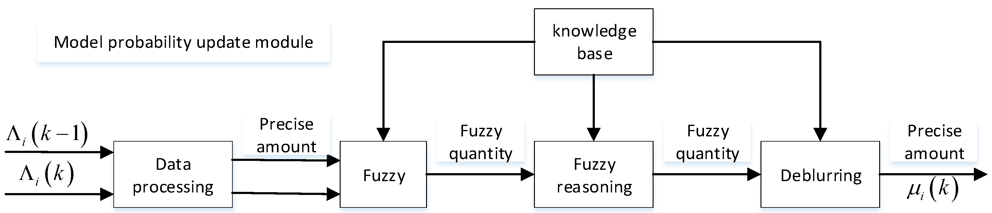
The fuzzy logic algorithm is used to update the model probability [
24], so that the model probability is quickly converted to accelerate the response speed of the filtering system.
Figure 1 shows the structure of the fuzzy logic algorithm in the model probability update module.
In this paper, we use two kinds of maneuver models of constant velocity and “snake-like” to simulate, so the input of the filter of the model probability update module is
and
. Firstly, the model probabilities
and
, corresponding to the two models, are calculated according to the IMM algorithm to calculate the model probability.
It can be derived from Formulas (1)–(3):
In the formula
where
is the transition probability of the model
to
, and
is the probability of the first model,
is the probability of IMM update, and
c is the normalization constant.
Analyze model 1 (uniform linear motion), assuming that the input variables obtained by the model probability update module are
and
, and the resulting output variable is
, let
- (1)
The domain of input variables and output variables:
- (2)
Fuzzy set of input variables and output variables:
- (3)
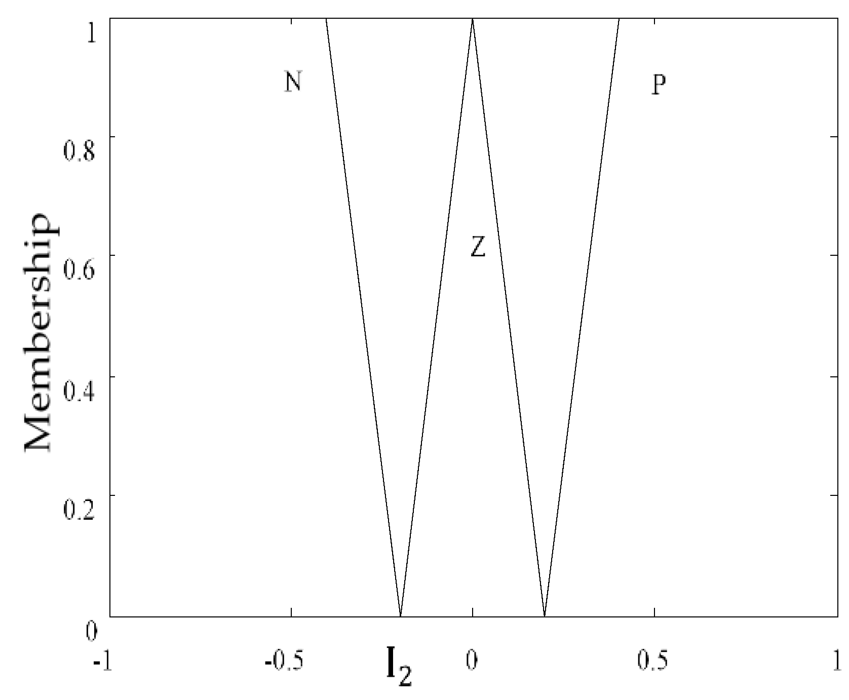
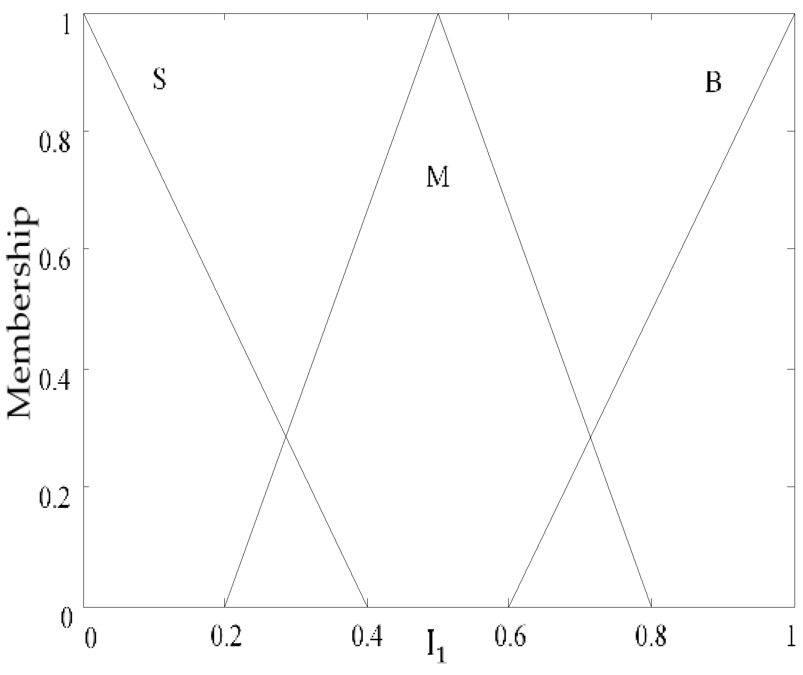
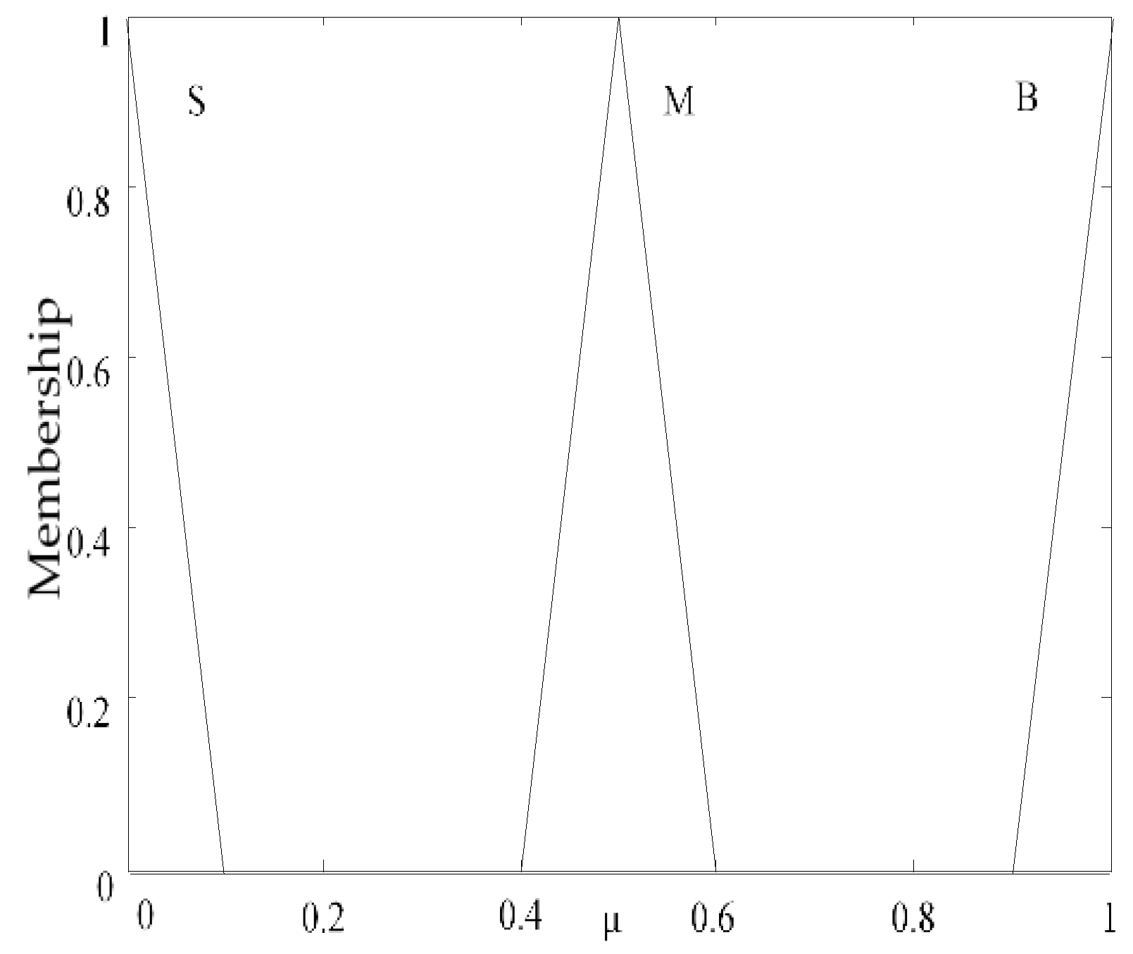
Determining the membership function:
Refer to
Figure 2,
Figure 3 and
Figure 4 to formulate fuzzy rules,
represents the probability of model 1 at
moment,
represents the difference between the updated probability and the pre-update probability after updating at the moment of l.
is the probability of time
, then, analyze these three variables: if
is a negative value and is denoted as N, then the probability
at k moment must be smaller than the model probability
at
moment; if
is equal to 0, it is recorded as Z, then the probability
at k moment should be equal to the model probability
at
moment; if
is a positive value and is denoted as P, then the probability
at l moment must be greater than the model probability
at
moment. Their fuzzy logic rules are shown in
Table 1:
When the output of the fuzzy logic system is defuzzified, the median method is used to defuzzify and obtain the actual probability of the model.
3. Adaptive Five-Degree Cubature Kalman
In order to pursue the better performance of the 5CKF filtering algorithm [
16,
17], the error covariance is improved based on the principle of Sage–Husa noise estimator, and a five-degree cubature Kalman algorithm based on error covariance adaptive is proposed.
Assume random variable x, its mean is , is its covariance matrix, the A5CKF algorithm consists of two parts: time update and measurement update.
3.1. Time Update
(1) Performing Cholesky decomposition on the covariance matrix
:
(2) Calculate the cubature point:
where the dimension of the system is
n; the weight of the cubature point is
,
, and
; and the unit vector is
.
(3) Propagating the cubature point:
Substituting the cubature point into the equation of state to obtain the cubature point after propagation.
(4) Prediction of state values:
Calculate the predicted value by combining the transmitted sample points with the corresponding weighted values.
(5) Prediction of the state error covariance matrix:
3.2. Measurement Update
(1) Performing Cholesky decomposition on the prediction covariance matrix
:
(2) Calculate the cubature point:
(3) Propagating the cubature point:
Substituting the cubature point into the observation equation to obtain the cubature point after propagation.
(4) Predicted observation:
Calculating the observed values by weighted summation of the propagated cubature points.
(5) Prediction of the error covariance matrix:
Calculating the predicted error covariance matrix by weighted summation.
(6) Calculation of the cross-covariance matrix:
Calculating the cross-covariance matrix by weighted summation.
(7) Estimate the Kalman gain:
(8) Estimate the updated state:
(9) Update of covariance matrix:
(10) Calculation of residuals:
(11) Recursive estimation
statistical characteristics:
4. Algorithm Overall Framework
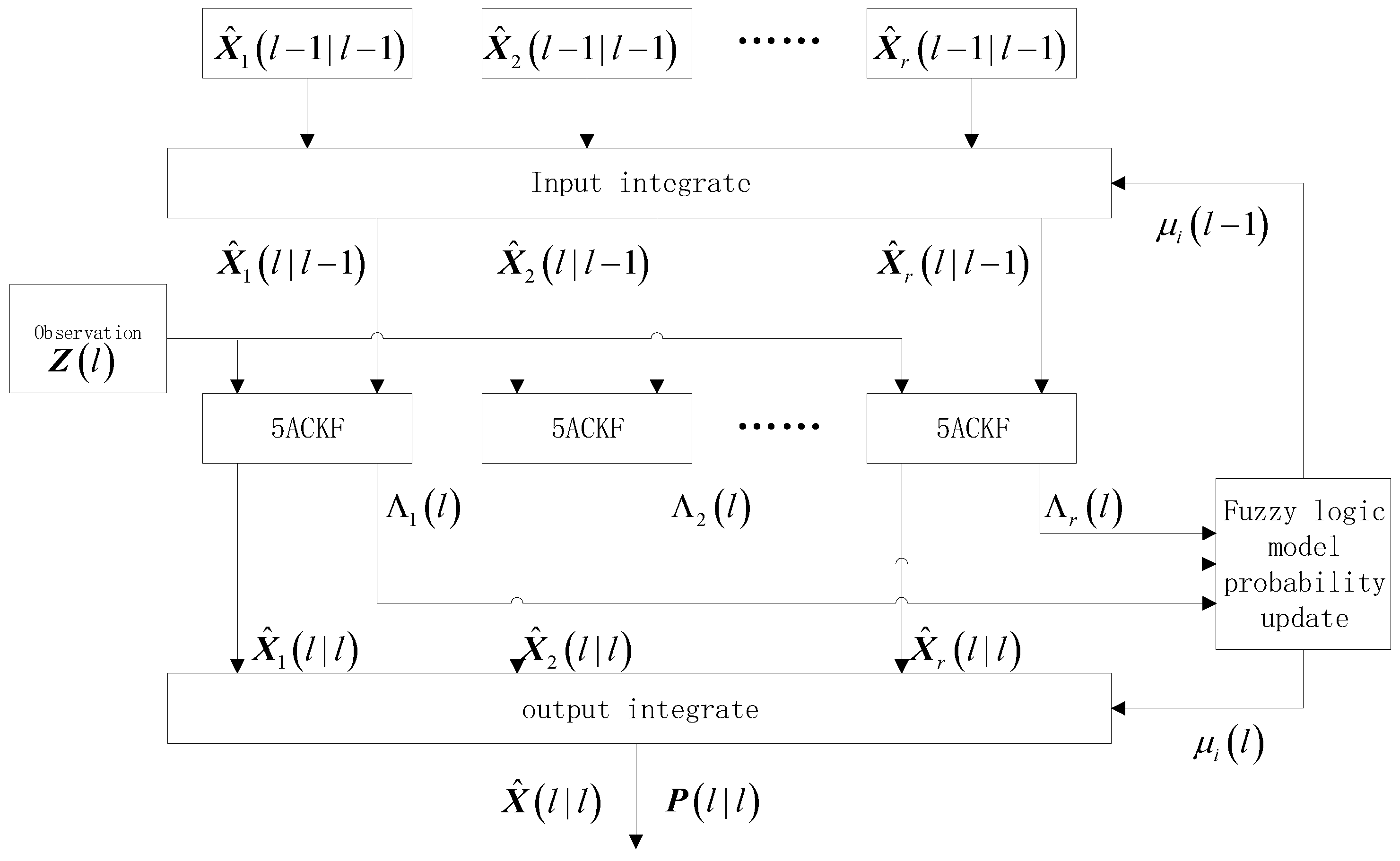
In order to obtain good filtering accuracy and response speed, A5CKF and FL algorithms are added in IMM, and an interactive multimodel adaptive five-degree cubature Kalman algorithm based on FL algorithm is proposed, which has the advantages of three algorithms. In the FLIMMA5CKF algorithm, the A5CKF filter is used for parallel filtering, the obtained estimation values are weighted and fused, and finally the state estimation is output. The execution steps of the FLIMMA5CKF algorithm and the IMM algorithm are basically the same: it is divided into four steps: input interaction, parallel filtering, update probability, and output data fusion.
Figure 5 below is the frame diagram of FLIMMA5CKF.
4.1. Input Interaction
Estimating the current time measurement value
according to the system state estimation and covariance estimation at the previous moment, and then performing a new initialization calculation on the model, wherein the new initial value is obtained by the Markov matrix between different models. Set the state optimal estimate and the estimated covariance matrix at model time
:
The following is the corresponding meaning: at time , for model , its conditional probability is , its probability is , its mathematical expectation is , and its error covariance is .
4.2. Parallel Filtering
The choice of filtering algorithm can also directly determine the tracking effect. Therefore, the parallel filtering module selects the A5CKF algorithm proposed in
Section 3 of this paper, which has better estimation effect. Then, based on the previously obtained a priori information combined with the execution steps of A5CKF, finally, we can get updated state variables and recursive estimation
statistical characteristics.
4.3. Update Probability
Model updating is also the key factor to determine the effectiveness of the algorithm. It uses maximum likelihood function combined with FL algorithm in this paper, and uses the principle of fuzzy logic to control the updating of model probability.
The likelihood function:
where the filter residual is represented by
, and the covariance matrix of the residual is
4.4. Output Data Fusion
According to the results of each model and their weights, the final output results are obtained.
6. Results and Discussion
Setting the same simulation conditions, the missile performs uniform linear motion in 0–15 s and snake motion in 16–60 s. Comparative analysis was performed using FLIMMA5CKF with IMMCKF, IMM5CKF, and IMMA5CKF algorithms.
The nonlinear observation equation of the target is described as follows:
where
is the observation vector,
is the measurement noise, and
is the observation function. The value is:
The performance of the four algorithms can be measured by the displacement, velocity, acceleration Error and RMSE at time l:
where m is the number of Monte Carlo simulations, n is the total number of sampling points,
is the true value, and
is the estimated value.
Assume that the target’s maneuvering frequency is
, the filtering period is 0.1 s, the Runge–Kutta method step size is 0.01 s, the initial probability of both models is 0.5, the initial state of the target is
, the initial state error covariance matrix is
, measuring noise standard deviation is 1 mrad, the standard noise standard deviation is 10, the Monte Carlo simulations are 50 times, and the transfer matrix between models is:
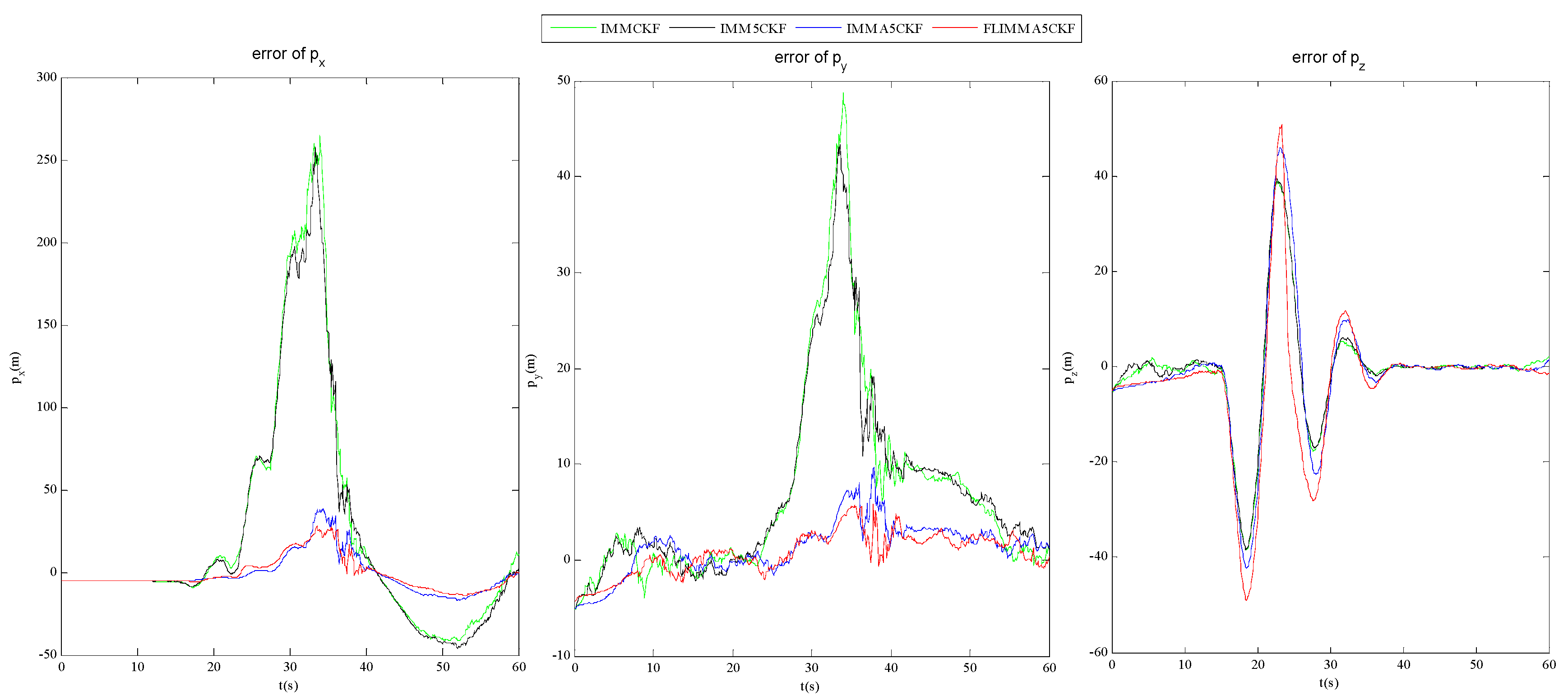
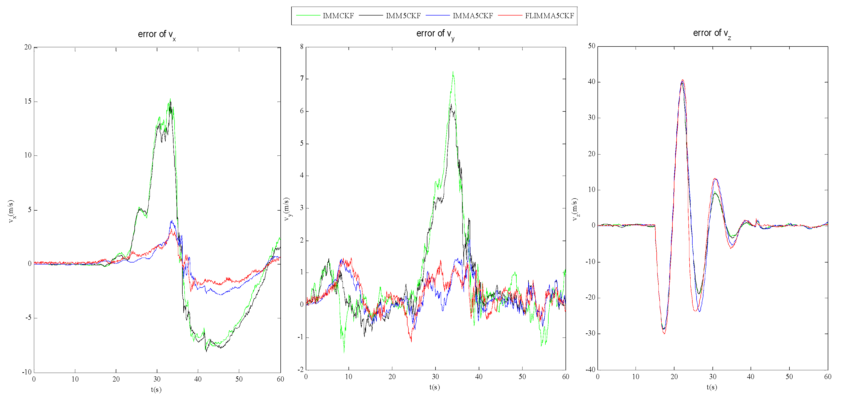
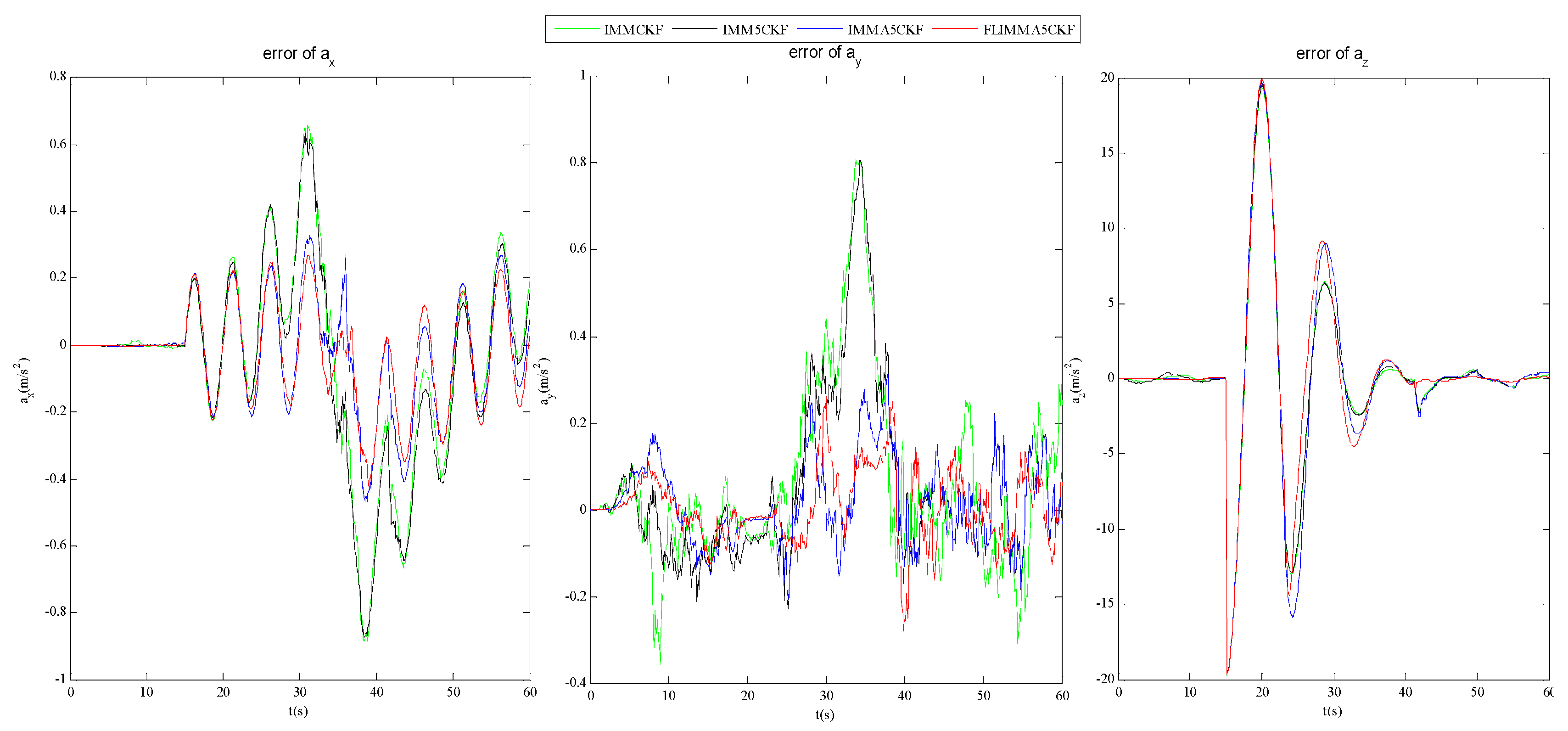
Figure 6,
Figure 7 and
Figure 8 are comparisons of error estimates for tracking targets using the improved FLIMMA5CKF algorithm, IMMA5CKF algorithm, IMM5CKF algorithm [
18], and IMMCKF algorithm [
14], respectively.
From
Figure 6,
Figure 7 and
Figure 8, combined with the data in
Table 2, it can be seen that the estimation error of the IMMA5CKF algorithm on the X-axis and the Y-axis is significantly smaller than the IMM5CKF algorithm of Zhu [
18], and the IMMCKF algorithm of Li [
14], which proves the high-precision characteristics of the A5CKF algorithm proposed in this paper, it not only adapts the error covariance, but also adapts the noise. Comparing the FLIMMA5CKF algorithm with IMMA5CKF, we can find that the estimation error of the FLIMMA5CKF algorithm is smaller than that of the IMMA5CKF algorithm. It proves that the FL algorithm proposed in this paper not only improves the accuracy of the algorithm, but also accelerates the convergence speed. In the Z-axis direction, the FLIMMA5CKF algorithm is slightly worse than the other three algorithms before 35 s, but after 35 s, the error reduction is obvious and more stable, in contrast, the other three algorithms have varying degrees of mutation or jump, in
Figure 6, the late estimation error is approximately
m, in
Figure 7, the late speed estimation error is ~0.4
, in
Figure 8, and the late acceleration estimation error is ~0.2
.
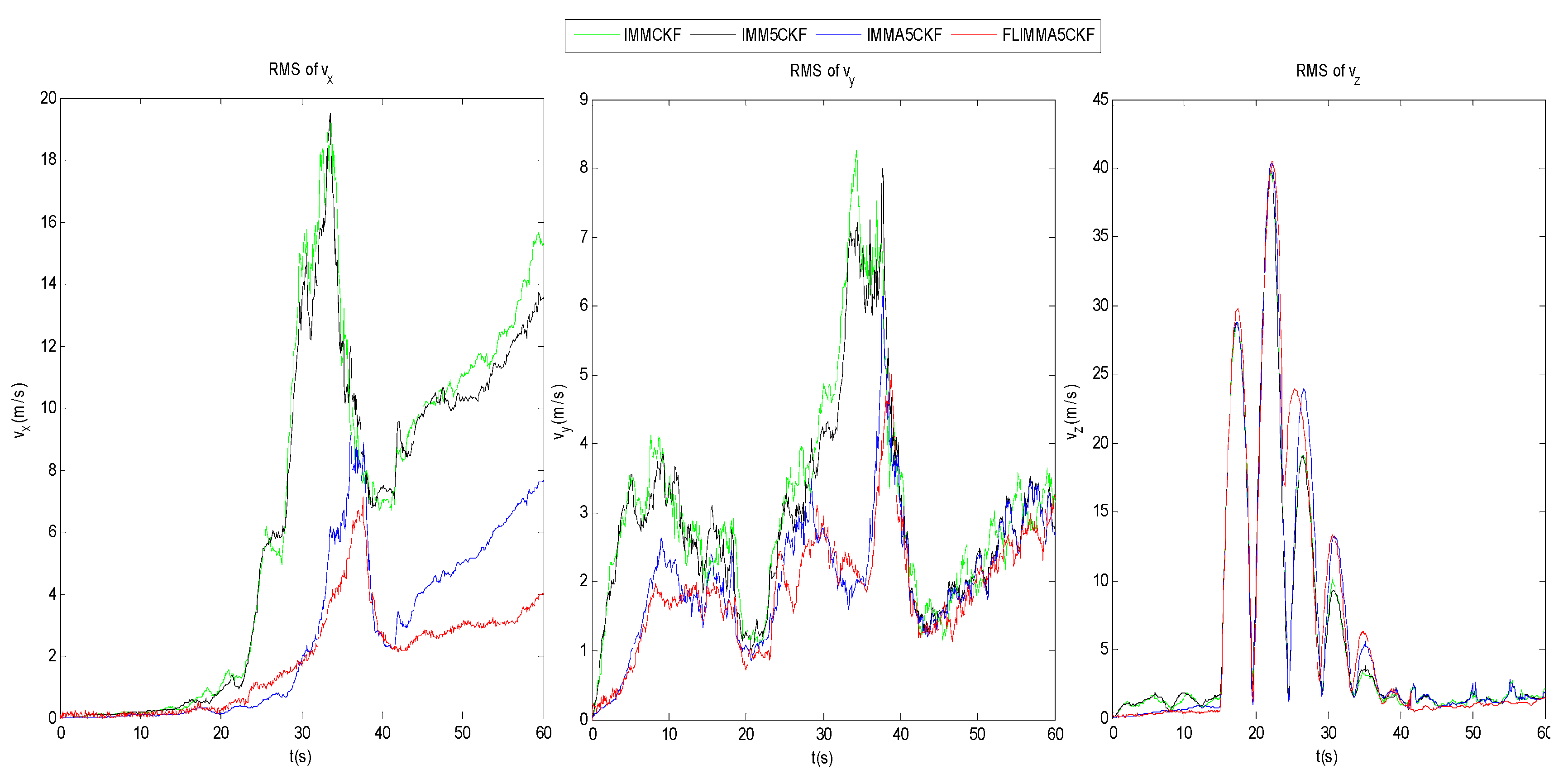
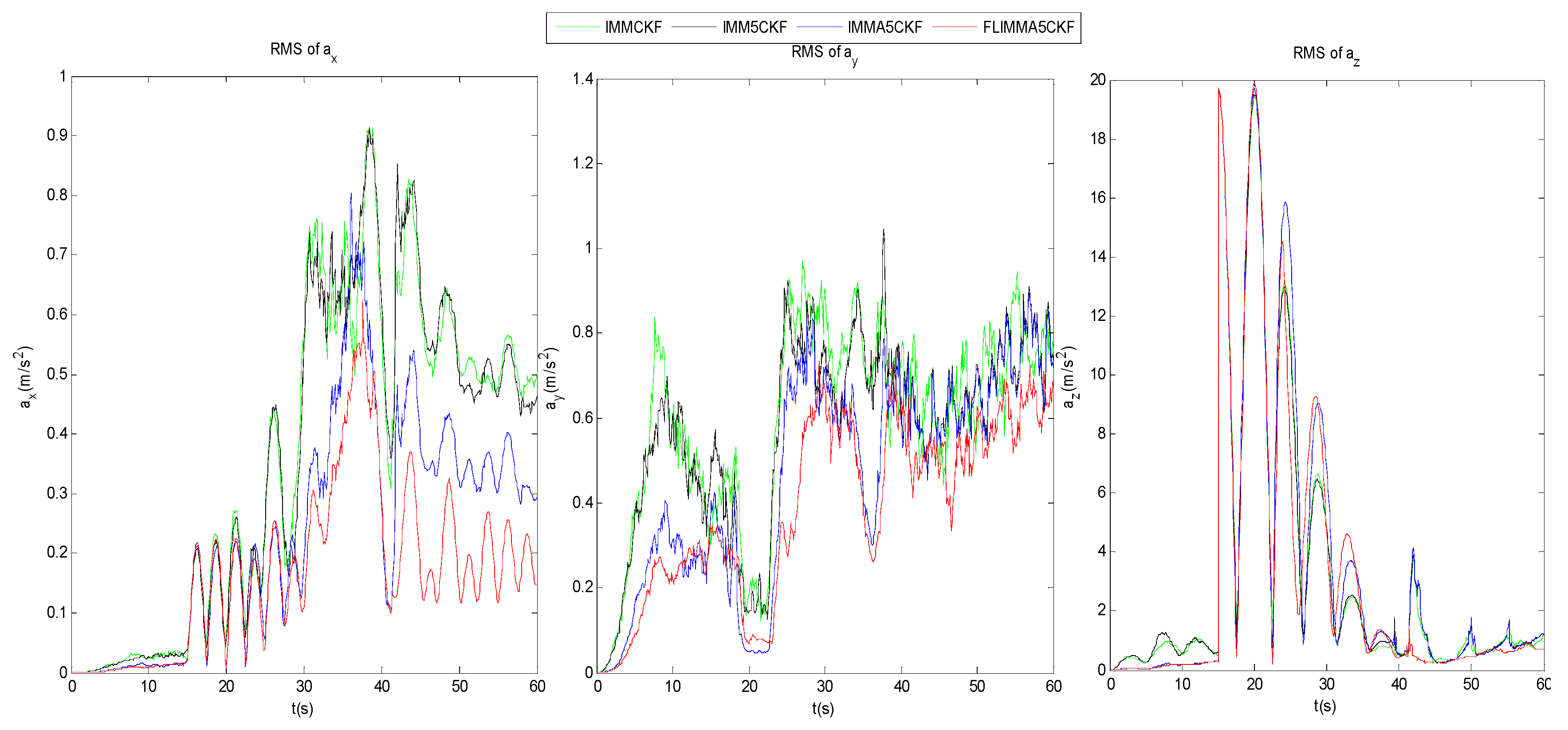
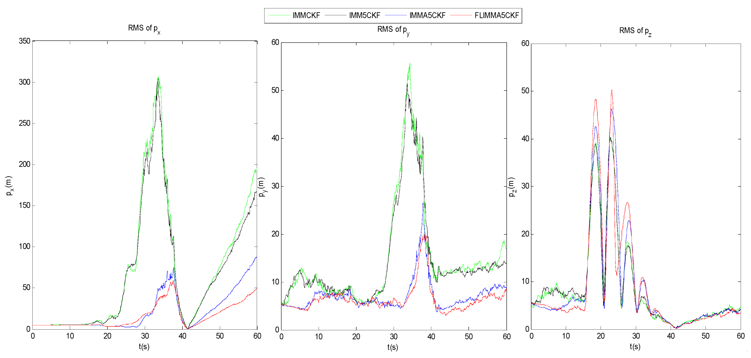
Figure 9,
Figure 10 and
Figure 11 shows the RMSE of the four algorithms. As can be seen from
Figure 9,
Figure 10 and
Figure 11, when the missile moves linearly at a constant speed, there is no significant difference in the tracking effect of several algorithms, but after 16 s, the missile begins to accelerate in a snake-like manner, as can be seen from
Figure 9,
Figure 10 and
Figure 11. Compared with the IMMCKF algorithm [
14], the IMM5CKF algorithm [
18], and the IMMA5CKF algorithm, the FLIMMA5CKF algorithm has a great improvement in tracking performance and stability. It can be seen from the Z-axis of
Figure 9,
Figure 10 and
Figure 11, FLIMMA5CKF has a better convergence speed than the other three algorithms, no peaks appear after 40 s, and the robustness is better.
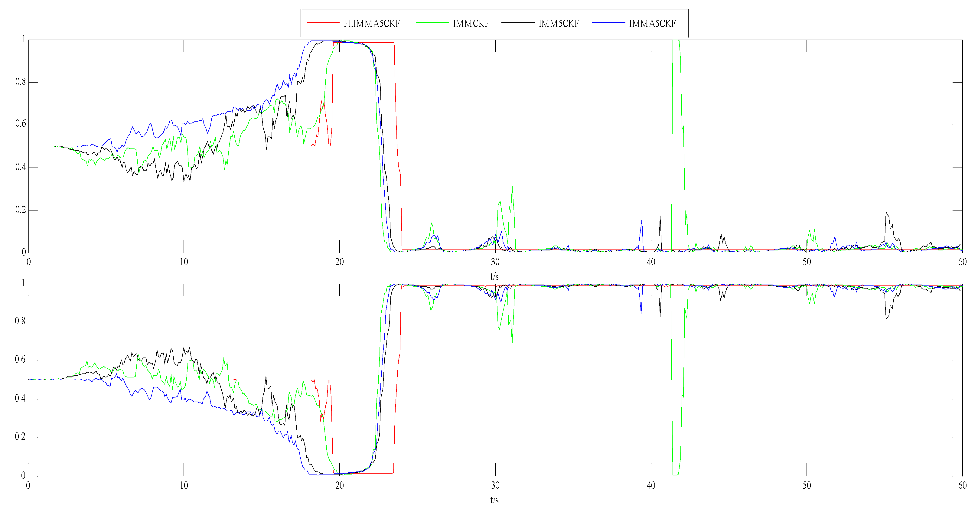
Figure 12 shows the model probability update graphs of the four algorithms, FLIMMA5CKF algorithm can better control model probability update due to the addition of fuzzy logic algorithm.
It can be seen from the data in
Table 3 that the performance of the FLIMMA5CKF algorithm in this paper is significantly higher than that of the IMMCKF algorithm [
14], IMM5CKF algorithm [
18], and IMMA5CKF algorithm in the X-axis and Y-axis directions. In the Z-axis direction, the algorithm of this paper is better than the other three, but the advantages of the algorithm are not particularly large. The shortcoming is that the FLIMMA5CKF algorithm in this paper is more complex than the other three algorithms, and the simulation time of the algorithm is relatively long.
7. Conclusions
Aiming at addressing the problem of poor filtering, slow convergence, and poor robustness in the IMM algorithm, this paper proposes the FLIMMA5CKF algorithm. The A5CKF algorithm is effective for improving the estimation effect, the FL algorithm can solve the problem of convergence speed very well, and these two algorithms are added to the IMM algorithm. By setting the same simulation model analysis, compared with IMMCKF, IMM5CKF, and IMMA5CKF, the proposed algorithm has a good filtering effect, and the hysteresis problem is also significantly improved. According to the analysis, in future research, the algorithm can take advantage of its accuracy to be used in actual positioning, tracking or navigation systems.


