Fast Calculation Method for Transient Response of Transmission Line Based on Chebyshev Pseudospectral–Two-Step Three-Order Boundary Value Coupled Method

Abstract

A Chebyshev pseudospectral–two-step three-order boundary value coupled method is proposed and presented for handling the issue associated with complicated calculation, low precision, and poor stability in the process of transient response of transmission line. The first order differential equation in time domain is obtained via dispersing the telegraph equation in space domain by utilizing the pseudospectral method (PSM) based on Chebyshev polynomial. Then the two-step three-order boundary value method (BVM3) is presented and employed to resolve the obtained differential equation, so the numerical solution of the space discrete points can be obtained. Furthermore, the Chebyshev pseudospectral–two-step three-order boundary value coupled method (PSM-BVM3) is presented and compared with the Chebyshev pseudospectral–two-step two order boundary value coupled method (PSM-BVM2), the pseudospectral–differential quadrature method (PSM-DQM), and the pseudospectral method–trapezoid rule (PSM-TR) to validate the feasibility of the new proposed method. Theoretical analysis and numerical simulation reveal that the proposed Chebyshev PSM-BVM3 has a higher performance than the conventional method. For the proposed Chebyshev PSM-BVM3, the higher precision, efficiency, and numerical stability can be obtained and achieved only with fewer discrete points in the space domain, which is suitable for solving the transient response of transmission line. The proposed PSM-BVM3 can improve the drawback of numerical instability of the PSM and can also improve the disadvantage of the BVM as it is not easy to change the latter’s timestep size.

1. Introduction

As the main carrier of information data of transmission line response, the research of transmission line response on excitation signal is significantly crucial in the electromagnetic transient analysis of transmission line. It is investigated that the transmission frequency of signal in high-speed and large-scale lumped circuit will gradually extend to high frequency and even ultra-high frequency [1,2]. Therefore, the issues of delay, distortion, and crosstalk caused by excitation signal passing through transmission line is becoming increasingly serious, which will directly influence the accuracy of transmission line response. As a result, in order to fully and accurately reflect the transient electromagnetic effect of the excitation signal passing through the transmission line, it is of great necessity to analyze the transient response process of transmission line.

Scholars have proposed many numerical methods to resolve the issues in transient response of transmission line, which mainly include the time domain analysis method and frequency domain analysis method. These methods mainly focused on solving the measurement-efficiency and precision problems of non-uniform multi-conductor transmission lines. Among them, Kokkinos et al. have proposed a finite difference time domain method (FDTD) that is simple and easy to implement and employ in practical applications but the calculation timestep of this method is constrained by the stability condition, which resulted in low computation efficiency [3,4]. Jiang et al. have proposed a precise integration method (PIM) that employed in the numerical calculation of telegraph equations in transient response process of transmission line [5,6]. PIM has the performance of good numerical stability and high precision as the calculation of numerical matrix exponent increases with the increase of system dimension. Feng et al. have proposed an improved FDTD (IFDTD) method that is has the higher calculation accuracy than the previous FDTD [7]. By using a time domain method that is similar to Maxwell’s equations, the modeling problem of transmission lines is resolved, and the accuracy of time domain solution is improved remarkably. However, as the calculation time step is quite small and the overall computation is accordingly increasing, it is hard to employ in practical applications. Xu et al. have applied the differential quadrature method (DQM) to transient response of transmission lines and the accuracy can be guaranteed due to its global approximation but with a complex calculation [8]. Hagci et al. have proposed a fast Fourier transform (FFT) method for calculating transient response of transmission line [9]. By using a high-order time-based function to approximate the transmission line parameters, it can preferably overcome electromagnetic interference and have good compatibility while bein susceptible to numerical dispersion and performing with deficiency. Thielen et al. have employed the convolution technique (CT) which shows that the instantaneous response of transmission line is calculated quickly, does not need to solve a large number of matrix equations, and has certain advantages in computation efficiency [10]. However, the stability is limited and numerical oscillation occurs easily. In general, the existing methods cannot take into full account stability, computation accuracy, and efficiency. Therefore, it is necessary to research the coupled algorithm with good comprehensive performance to analyze the transient response of transmission line.

Javidi et al. have proposed the pseudospectral method (PSM), which is also called spectral collocation method [11,12,13]. It is a numerical method widely used to resolve partial differential equation. The principle is to define a set of orthogonal functions as the basis function in the computation region, and then the basis function is used to approximate the resolved variable as its spectral approximation. Because PSM requires fewer discrete nodes to obtain higher approximation precision, Arribas et al. have successfully applied it in many fields. However, there are still some shortcomings for the PSM as the singularity of conventional PSM at the boundary will lead to numerical instability during the practical calculation [14,15,16]. Besides, most of the problems in engineering applications are non-periodic and the solution area is irregular, which will influence the calculation accuracy.

Truhlar et al. have proposed the boundary value method (BVM), Dahlquist et al. have studied the two-step boundary method, and Noor et al. have investigated the convergence and stability of the three and four step boundary value method. The results have shown BVM can control global error and has a high accuracy and great advantages in stability [17,18,19,20,21,22]. However, BVM still has some disadvantages such as its heavy and deficient calculation and it cannot change the step size. A synthesis of the transient response calculation approach proposed in the literature, depending on the type of analysis, is presented in

Table 1. Synthesis of transient response calculation approach. Finite difference time domain method (FDTD); precise integration method (PIM); improved FDTD (IFDTD); differential quadrature method (DQM); fast Fourier transform (FFT); convolution technique (CT); pseudo spectral method (PSM); boundary value method (BVM).

Transient Response Calculation Approach	Advantages	Drawbacks
FDTD	Simple and easy to implement and employ in practical application	Calculation timestep limitation, low computation efficiency
PIM	Good numerical stability, high precision	Calculation of numerical matrix exponent increase due to increase of system dimension
IFDTD	Higher calculation accuracy than conventional FDTD	Calculation burden due to its small calculation timestep
DQM	Accuracy can be guaranteed due to its global approximation	Complex calculation
FFT	Can preferably reduce electromagnetic interference and has good compatibility	Susceptible to numerical dispersion and performed with deficiency
CT	Good computation efficiency	Stability limitation, numerical oscillation
PSM	Requires fewer discrete nodes to obtain higher precision	Singularity at the boundary, non-periodic
BVM	High accuracy and great stability	Heavy and deficient calculation

.

By coupling the Chebyshev pseudospectral method and the boundary value method, a Chebyshev pseudospectral–two-step three-order boundary value coupled method is proposed and presented to resolve the transient response process of transmission line. Firstly, the first order differential equation in time domain is obtained by using the Chebyshev pseudospectral method to discrete telegraph equation in space domain, and then the equation is resolved by using the two-step three-order boundary value method, so the time domain solution of each discrete node can be obtained. Compared with the same level of pseudospectral–differential quadrature method and the Chebyshev pseudospectral–two-step two order boundary value coupled method, the simulation result shows that the coupled method proposed in this paper can simulate the transient response process of transmission line more accurately, and has high precision and efficiency. Moreover, it is unconditionally stable in the time domain, is no longer constrained by Courant conditions, and the spectral precision is convergent in space domain.

2. Chebyshev Pseudospectral Method

The p-order Chebyshev differential matrix ${\tilde{\mathit{D}}}_N^{\left(p\right)}$ is defined as:

$$\mathit{G}={\tilde{\mathit{D}}}_N^{\left(p\right)}\mathit{U}$$

(1)

where: $\mathit{G}={\left[g\left({\tilde{x}}_0\right),\cdots ,g\left({\tilde{x}}_N\right)\right]}^T$, ${\tilde{\mathit{D}}}_N^{\left(p\right)}={\left({\tilde{d}}_{ij}^{\left(p\right)}\right)}_{\left(N+1\right)\times \left(N+1\right)}$, $\mathit{U}={\left[u\left({\tilde{x}}_0\right),\cdots ,u\left({\tilde{x}}_N\right)\right]}^T$, ${\tilde{x}}_i=\cos \left(i\pi /N\right),i,j\in \left(0,N\right)$.

Babolian et al. have defined the formula of any element of the one-order Chebyshev differential matrix when $p=1$, as shown in Formula (2) [23,24,25,26,27]. And the two-order Chebyshev differential matrix can be directly obtained as shown in Formula (3).

$$\{\begin{array}{l}{\tilde{d}}_{00}^{\left(1\right)}=-{\tilde{d}}_{NN}^{\left(1\right)}=\left(2N^2+1\right)/6\\ {\tilde{d}}_{ij}^{\left(1\right)}=-\frac{{\gamma }_i}{2{\gamma }_j}\frac{{\left(-1\right)}^{i+j}}{\sin \left(\left(i+j\right)\frac{\pi }{2N}\right)\sin \left(\left(i-j\right)\frac{\pi }{2N}\right)},i\ne j\\ {\tilde{d}}_{ij}^{\left(1\right)}=-\frac{1}{2}\cos \left(\frac{i\pi }{N}\right)\left(1+{\cot }^2\left(\frac{i\pi }{N}\right)\right),i=j,i\ne 0,N\\ {\gamma }_k=\{\begin{array}{l}2,k=0,N\\ 1,k\in \left(1,N-1\right)\end{array}\end{array}$$

(2)

$${\tilde{\mathit{D}}}_N^{\left(2\right)}={\tilde{\mathit{D}}}_N^{\left(1\right)}{\tilde{\mathit{D}}}_N^{\left(1\right)}$$

(3)

As can be known that the Chebyshev point $x_i$ in the general interval $[a,b]$ can be obtained by simple linear transformation as shown in Formula (4). Where, $i\in \left(0,N\right)$.

$$x_i=a+\frac{b-a}{2}\left({\tilde{x}}_i+1\right)$$

(4)

Accordingly, the Chebyshev differential matrix ${\mathit{D}}_N^{\left(p\right)}$ corresponding to Chebyshev point $x_i$ in any interval $[a,b]$ can be given as:

$${\mathit{D}}_N^{\left(p\right)}={\left(\frac{2}{b-a}\right)}^p{\tilde{\mathit{D}}}_N^{\left(p\right)}$$

(5)

For simplicity, the above method is called Chebyshev pseudospectral method in the following text.

3. Two-Step Three-Order Boundary Value Method

Consider the initial value problem of the following first-order ordinary differential equation:

$$\{\begin{array}{l}\dot{\mathit{y}}\left(t\right)=\mathit{f}\left(t,\mathit{y}\left(t\right)\right),t\in \left(t_0,t_f\right)\\ \mathit{y}\left(t_0\right)={\mathit{y}}_0,\end{array}$$

(6)

The two-step boundary value method is used to solve the first-order ordinary differential equation as shown in Formula (6). In addition, the calculation form of the two-step two-order boundary value method is shown in Formula (7).

$${\mathit{y}}_{m+1}-\left(1+\beta \right){\mathit{y}}_m+\beta {\mathit{y}}_{m-1}=\frac{h}{2}[\left(3-\beta \right){\mathit{f}}_m-\left(1+\beta \right){\mathit{f}}_{m-1}],m\in \left(1,M-1\right)$$

(7)

In the same way, Dahlquist et al. [19] gave the calculation equation of the two-step three-order boundary value method and is shown in Formula (8).

$${\mathit{y}}_{m+1}-\left(1+\theta \right){\mathit{y}}_m+\theta {\mathit{y}}_{m-1}=\frac{h}{12}[\left(5+\theta \right){\mathit{f}}_{m+1}+8\left(1-\theta \right){\mathit{f}}_m-\left(1+5\theta \right){\mathit{f}}_{m-1}],m\in \left(1,M-1\right)$$

(8)

In Formulas (7) and (8), h is the length of the time-integral step, and M is the number of time intervals. Where, $h\equiv t_{m+1}-t_m=\left(t_f-t_0\right)/M$, ${\mathit{f}}_{m+i}=\mathit{f}\left(t_{m+i},{\mathit{y}}_{m+i}\right),i=-1,0,1$, ${\mathit{y}}_{m+i}=\mathit{y}\left(t_{m+i}\right)$, $t_{m+i}=t_m+i\times h$.

In Formulas (7) and (8), if we attempt to resolve the unknown points ${\mathit{y}}_1,{\mathit{y}}_2,\cdots ,{\mathit{y}}_{M-1}$, the two boundary values ${\mathit{y}}_0,{\mathit{y}}_M$ must be obtained. For the initial value problem (6), only ${\mathit{y}}_0$ is known. Therefore, the additional equation should be introduced to solve the unknown point ${\mathit{y}}_M$.

$${\mathit{y}}_M={\mathit{y}}_{M-1}+\frac{h}{2}({\mathit{f}}_M+{\mathit{f}}_{M-1})$$

(9)

Combining Formulas (7) or (8) and (9) to resolve the initial value question (6), we can get the value of each time discrete point ${\mathit{y}}_k,k\in \left(1,M\right)$.

4. Calculation Method for Transient Response of Transmission Line Based on Chebyshev Pseudospectral–Two-Step Three-Order Boundary Value Coupled Method

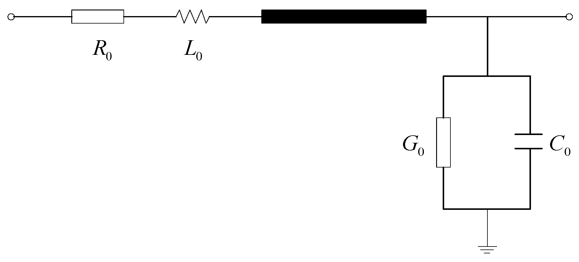
Topology Model of a single uniform transmission line is shown in Figure 1. In Figure 1, $R_0$, $L_0$, $G_0$, and $C_0$ are the resistance, inductance, conductance, and capacitance per unit length of the single uniform transmission line, respectively.

The famous telegraph equations known to describe voltage and current variations on a uniform transmission line can be written as:

$$\frac{{\partial }^2\omega \left(z,t\right)}{\partial t^2}+k_0\frac{\partial \omega \left(z,t\right)}{\partial t}=a_0^2\frac{{\partial }^2\omega \left(z,t\right)}{\partial z^2}+b_0\omega \left(z,t\right)$$

(10)

where, $a_0=\frac{1}{\sqrt{L_0{C}_0}}$, $b_0=-\frac{R_0{G}_0}{L_0{C}_0}$, $k_0=\frac{G_0{L}_1+C_0{R}_1}{C_0{L}_1}$.

The new variable $\omega \left(z,t\right)$ represents the voltage or current of the transmission line. The definition domain is $\left(z,t\right)\in \left[c,d\right]\times \left[0,T\right]$, and the initial conditions are:

$$\omega \left(z,0\right)={\upsilon }_1\left(z\right),\begin{array}{cc}& \end{array}z\in \left[c,d\right]$$

(11)

$${\omega }_t\left(z,0\right)={\upsilon }_2\left(z\right),\begin{array}{cc}& \end{array}z\in \left[c,d\right]$$

(12)

The Dirichlet boundary conditions are:

$$\omega \left(c,t\right)=h_1\left(t\right),\begin{array}{cc}& \end{array}t\in \left[0,T\right]$$

(13)

$$\omega \left(d,t\right)=h_2\left(t\right),\begin{array}{cc}& \end{array}t\in \left[0,T\right]$$

(14)

By multiplying $e^{-k_{0}t/2}$ in both sides of Equation (10), the equation can be simplified as:

$$\frac{{\partial }^2\varpi \left(z,t\right)}{\partial t^2}=a_0^2\frac{{\partial }^2\varpi \left(z,t\right)}{\partial z^2}+\left(b_0+\frac{1}{4}{k}_0^2\right)\varpi \left(z,t\right)$$

(15)

In Formula (15), $\varpi \left(z,t\right)=e^{k_{0}t/2}\omega \left(z,t\right)$, the definition domain of the new variable is not changing, and the initial conditions are:

$$\varpi \left(z,0\right)={\upsilon }_1\left(z\right),\begin{array}{cc}& \end{array}z\in \left[c,d\right]$$

(16)

$${\varpi }_t\left(z,0\right)={\upsilon }_2\left(z\right)+\frac{1}{2}{k}_0{\upsilon }_1\left(z\right),\begin{array}{cc}& \end{array}z\in \left[c,d\right]$$

(17)

The Dirichlet boundary condition is changed to:

$$\varpi \left(c,t\right)=e^{k_{0}t/2}{h}_1\left(t\right),\begin{array}{cc}& \end{array}t\in \left[0,T\right]$$

(18)

$$\varpi \left(d,t\right)=e^{k_{0}t/2}{h}_2\left(t\right),\begin{array}{cc}& \end{array}t\in \left[0,T\right]$$

(19)

By using Chebyshev pseudospectral method, the ${\varpi }_{zz}$ in Formula (15) can be dispersed as formula as:

$${\varpi }_{zz}\left(z_i,t\right)={\displaystyle \sum _{j=0}^N{d}_{ij}^{\left(2\right)}}\varpi \left(z_j,t\right),\begin{array}{cc}& \end{array}i\in \left(0,N\right)$$

(20)

where, $d_{ij}^{\left(2\right)}={\left(\frac{2}{d-c}\right)}^2{\tilde{d}}_{ij}^{\left(2\right)}$, $z_i=c+\frac{d-c}{2}\left({\tilde{x}}_i+1\right)$. Substituting Formula (20) into Formula (15), we can get:

$$\frac{{\mathrm{d}}^2\mathit{\varpi }}{\mathrm{d}{t}^2}=\left[a_0^2{\mathit{D}}_N^{\left(2\right)}+\left(b_0+\frac{1}{4}{k}_0^2\right){\mathit{I}}_{N+1}\right]\mathit{\varpi }$$

(21)

where, $\mathit{\varpi }={\left[\varpi \left(z_i,t\right)\right]}^T$, $i\in \left(0,N\right)$. ${\mathit{I}}_{N+1}$ is a $N+1$ dimensional identity matrix. Define the following vector $\mathit{\zeta }$, and let $\mathit{\vartheta }=\frac{\mathrm{d}\mathit{\varpi }}{\mathrm{d}t}$:

$$\mathit{\zeta }=\left[\begin{array}{c}\mathit{\vartheta }\\ \mathit{\varpi }\end{array}\right]$$

(22)

Then the following initial value problem can be obtained:

$$\{\begin{array}{l}\dot{\mathit{\zeta }}=\Delta \mathit{\zeta }\begin{array}{cc}& \end{array},t\in \left(0,T\right]\\ \mathit{\zeta }\left(t=0\right)={\mathit{\zeta }}_0\end{array}$$

(23)

in Formula (23),

$$\Delta =\left(\begin{array}{cc}0& \mathit{P}\\ \mathit{\Gamma }& 0\end{array}\right)$$

(24)

in Formula (24), $\mathit{P}=a_0^2{\mathit{D}}_N^{\left(2\right)}+\left(b_0+\frac{1}{4}{k}_0^2\right){\mathit{I}}_{N+1}$, and $\mathit{\Gamma }$ is the $N+1$ dimensional identity matrix.

The first-order ordinary differential initial value model for transient response calculation of transmission line is obtained. By using the two-step three-order boundary value method as the basic method, and using the implicit trapezoid formula as the last point method, the global discrete solution of Formula (23) in the time domain can be carried out, and the following equations can be obtained:

$${\mathit{J}}_0\mathit{\zeta }=\mathit{{\rm Z}}$$

(25)

in Equation (25), ${\mathit{J}}_0$ is a constant coefficient matrix, $q=2(N+1)$, $i\in (1,M)$. The form of each variable is:

$$\mathit{\zeta }\equiv {\left[{\mathit{\xi }}_1^{\mathrm{T}},{\mathit{\xi }}_2^{\mathrm{T}},\cdots ,{\mathit{\xi }}_M^{\mathrm{T}}\right]}^{\mathrm{T}},{\mathit{\xi }}_i\in {\mathrm{R}}^{q\times 1}$$

(26)

$$\mathit{{\rm Z}}\equiv {\left[{\mathit{z}}_1^{\mathrm{T}},{\mathit{z}}_2^{\mathrm{T}},\cdots ,{\mathit{z}}_M^{\mathrm{T}}\right]}^{\mathrm{T}},{\mathit{z}}_i\in {\mathrm{R}}^{q\times 1}$$

(27)

$${\mathit{J}}_0=\left[\begin{array}{ccccc}{\mathit{J}}_1& {\mathit{J}}_5& & & 0\\ {\mathit{J}}_3& {\mathit{J}}_1& {\mathit{J}}_5& & \\ & \ddots & \ddots & \ddots & \\ & & {\mathit{J}}_3& {\mathit{J}}_1& {\mathit{J}}_5\\ 0& & & {\mathit{J}}_4& {\mathit{J}}_2\end{array}\right]$$

(28)

in Formula (28):

$${\mathit{J}}_1=-\left[\left(1+\theta \right){\mathit{I}}_q+\frac{2\left(1-\theta \right)}{3}h\Delta \right]$$

(29)

$${\mathit{J}}_2=\left({\mathit{I}}_q-\frac{1}{2}h\Delta \right)$$

(30)

$${\mathit{J}}_3=\left[\theta {\mathit{I}}_q+\frac{\left(1+5\theta \right)}{12}h\Delta \right]$$

(31)

$${\mathit{J}}_4=-\left({\mathit{I}}_q+\frac{1}{2}h\Delta \right)$$

(32)

$${\mathit{J}}_5=\left[{\mathit{I}}_q-\frac{\left(5+\theta \right)}{12}h\Delta \right]$$

(33)

where, ${\mathit{I}}_q$ is a q-order identity matrix.

As can be seen from the above derivation, if Gauss elimination is directly used to solve Equation (25), the trig decomposition of a $q\times M$ dimensional matrix will be involved. In this way, the calculated amount is about $2q^3{M}^3/3$ times multiplication and division without considering the sparsity of ${\mathit{J}}_0$. However, because ${\mathit{J}}_0$ is a large dimensional block tridiagonal matrix, the catch-up method for a block tridiagonal matrix equation is applied to solve this equation [28]. In this case, the calculated amount can be reduced to $2M{q}^3/3+2M{q}^2$. As a contrast, the s-step s-order differential quadrature method based on network uniformity and fast numerical algorithm based on V-conversion are used to solve the initial value problem (23). Danesh et al. have presented the calculation process and calculation amount of this method in detail, which is not repeated in this paper [29]. Through comparison, the advantages of the proposed algorithm in calculation precision and efficiency can be further illustrated. The final point method is the same, and only ${\mathit{J}}_0$ should be adjusted accordingly.

5. Simulation Test

For different values of parameters in Equation (10), two examples are given to validate the improved performance of the proposed algorithm. The Chebyshev pseudospectral–two-step two-order boundary value coupled method (PSM-BVM2), the Chebyshev pseudospectral–two-step three-order boundary value coupled method (PSM-BVM3), and the Chebyshev pseudospectral–two-step differential quadrature method (PSM-DQM2) are adopted to solve the initial value problem (23), to validate the performance of the proposed method. All three methods are approximated dispersing by the Chebyshev pseudospectral method in space domain and adopting the same step size h in time domain. The simulation software is Matlab7.14, and the hardware platform is CPU Intel core i7-8700k 3.70 GHz.

5.1. Test for Example 1

In Equation (10), $a_0=2$, $b_0=-3{\pi }^2$, $k_0=8\pi$, $c=0$, $d=1$. The initial value and Dirichlet boundary condition are determined by analytic solution of $\omega \left(z,t\right)=e^{-\pi t}\sin \left(\pi z\right)$. Here the PSM-BVM2 $\left(\beta =-6\right)$, PSM-BVM3 $\left(\theta =-3\right)$, and PSM-DQM2 are used to resolve the initial value problem (23). The spatial discrete points of the Chebyshev pseudospectral method are $N^{\prime }$. The absolute error (AE) and relative error (RE) were compared.

In order to test the computational accuracy of the proposed algorithm, different simulation times are selected using the analytic solution as the benchmark. The numerical errors of the above algorithms are compared and analyzed. As shown in

Table 2. The calculation error of the Chebyshev pseudospectral–two-step two-order boundary value coupled method (PSM-BVM2, the Chebyshev pseudospectral–two-step three-order boundary value coupled method (PSM-BVM3), and the Chebyshev pseudospectral–two-step differential quadrature method (PSM-DQM2). $\left(N^{\prime }=8,h=0.1 \mathrm{ms}\right)$.

$\mathit{T}$ (s)	PSM-BVM2 $(\times {10}^{-8})$		PSM-BVM3 $(\times {10}^{-11})$		PSM-DQM2 $(\times {10}^{-8})$
	AE	RE	AE	RE	AE	RE
0.5	4.3670	8.4341	3.1342	6.2379	5.2916	9.0227
1	1.5147	8.7979	1.1578	6.4569	1.9340	9.6047
2	0.1238	8.8508	0.1058	6.5736	0.1605	9.6879

and

Table 3. The calculation error of PSM-BVM3, PSM-BVM2 and PSM-DQM2. $\left(N^{\prime }=12,h=0.1 \mathrm{ms}\right)$.

$\mathit{T}$ (s)	PSM-BVM2 $(\times {10}^{-8})$		PSM-BVM3 $(\times {10}^{-11})$		PSM-DQM2 $(\times {10}^{-8})$
	AE	RE	AE	RE	AE	RE
0.5	2.8129	4.1365	1.2515	2.9344	7.4130	6.2612
1	1.9138	5.3662	0.9821	3.5907	3.0820	7.6619
2	0.1017	5.7901	0.1048	3.6808	0.2664	7.8543

, the results of the PSM-BVM2, PSM-BVM3, and PSM-DQM2 are given.

From Table 2 and Table 3, it can be seen that the measurement error of the PSM-BVM3 and the PSM-BVM2 are less than that of the PSM-DQM2, which can prove that the proposed PSM-BVM algorithm exhibits improved performance. Moreover, the measurement error of the PSM-BVM3 is three times less than that of the PSM-DQM2 and the PSM-BVM2. In conclusion, according to the result, the PSM-BVM3 has higher accuracy than the other two algorithms of the PSM-BVM2 and the PSM-DQM2.

To validate the computation efficiency of the proposed algorithm, the CPU consumption time of the above three methods was tested under different spatial discrete points, as shown in

Table 4. Comparison of CPU consumption time between three algorithms.

${\mathit{N}}^{\prime }$	PSM-BVM2	PSM-BVM3	PSM-DQM2
8	0.936 s	1.172 s	5.386 s
12	1.013 s	1.948 s	5.742 s

. In Table 4, $T=2 \mathrm{s}$, $h=0.1 \mathrm{ms}$.

From Table 4, it can be seen that the average CPU consumption time is 0.9745 s for the PSM-BVM2, 1.560 s for the PSM-BVM3, and 5.564 s for the PSM-DQM2, which indicated that the PSM-BVM3 and PSM-BVM2 have higher computation efficiency. Moreover, the runtime of the PSM-BVM3 is larger than the PSM-BVM2. But considering the measurement accuracy and the runtime cost, the PSM-BVM3 exhibits the most improved performance than the PSM-DQM2 and the PSM-BVM2, which can prove that the higher runtime required by PSM-BVM3 (see Table 4) is justified by an improvement in the quality of the solutions.

5.2. Test for Example 2

In Equation (10), $a_0=1/\pi$, $b_0=-4$, $k_0=4$,$c=0$, $d=1$. In the same way, the initial value and Dirichlet boundary condition are determined by analytic solution of $\omega \left(z,t\right)=e^{-t}\cosh \left(\pi z\right)$. The number of spatial discrete points is $N^{″}=14$. $h=0.001 \mathrm{s}$, $T=15 \mathrm{s}$. Here the PSM-BVM2 $\left(\beta =-6\right)$ and PSM-BVM3 $\left(\theta =-3\right)$ are used to solve, by using the analytic solution of (10) as the benchmark. The absolute error of the two methods $err\left(z,t\right)=\left|\tilde{\omega }\left(z,t\right)-\omega \left(z,t\right)\right|$ are tracked, where $\tilde{\omega }$ is the numerical solution. 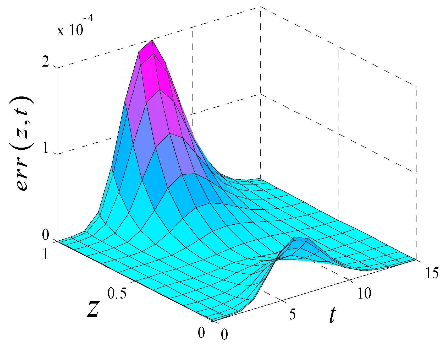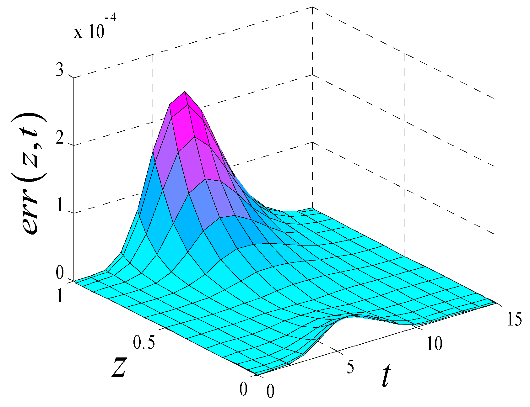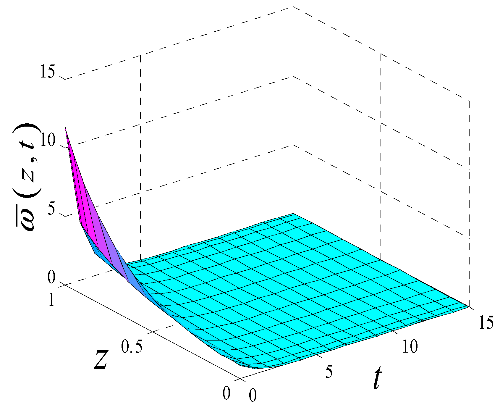The error curves are shown in Figure 2 and Figure 3. The numerical results of PSM-BVM3 $\overline{\omega }\left(z,t\right)$ and analytical solutions of example 2 are shown in Figure 4 and Figure 5. Only part of sample points are intercepted in Figure 2, Figure 3, Figure 4 and Figure 5.

From Figure 2 and Figure 3 we can see that both the PSM-BVM2 and PSM-BVM3 can well track the transient response process of analog transmission lines, and the calculation errors are generally decreasing with the change of time, so the algorithm has good convergence. In the time domain, the PSM-BVM3 has better calculation accuracy than the PSM-BVM2.

From Figure 4 and Figure 5, the numerical results of the PSM-BVM3 are almost the same as the real analytical solutions, which fully shows that the algorithm is unconditionally stable in the time domain and the spectral precision is convergent in the space domain.

In conclusion, the example 1 shows that the PSM-BVM2 and PSM-BVM3 are more accurate and efficient than the PSM-DQM2, and example 2 shows that the numerical stability of the proposed algorithm can be guaranteed after long time integration process. Therefore, compared with the PSM-DQM2, PSM-BVM2, and PSM-BVM3 have higher precision and efficiency, and good numerical stability, so they can simulate the transient response process of transmission line for a long time.

5.3. Calculation of Transient Response of Nondestructive Transmission Line

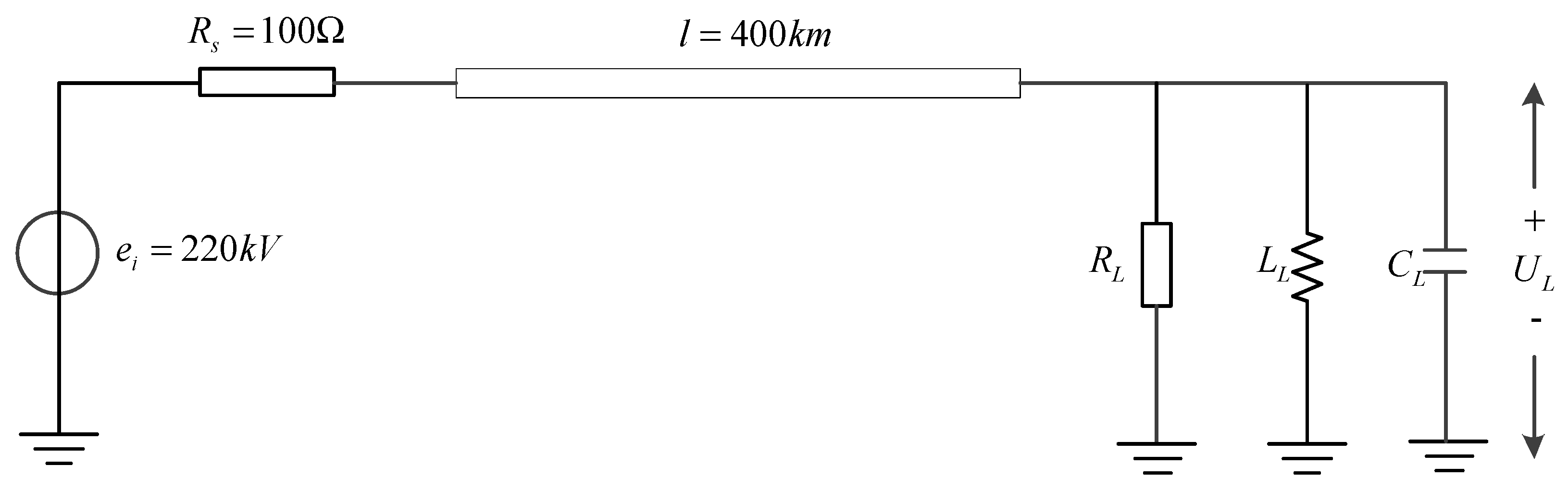
In order to validate the feasibility and effectiveness of the proposed coupled method in practical cases, the example of the transient response of transmission line is carried out, in which the comparison between the PSM-BV3, PSM-BVM2 and the pseudospectral method–trapezoid rule (PSM-TR) is presented.

The simulation circuit diagram of nondestructive transmission line is shown in Figure 6. And the parameters of the transmission are set as:

The excitation source is a step voltage source $e_i=100\epsilon (t) \mathrm{kV}$ where $\epsilon (t)$ is a unit step function. The internal resistance of source is $R_S=100 \mathsf{\Omega }$. The transmission line length is $l=400 \mathrm{km}$, and the distribution parameters of transmission line are $L_0=2.5\times {10}^{-7}\mathrm{H}/\mathrm{m}$, $C_0=1.0\times {10}^{-10}\mathrm{F}/\mathrm{m}$. The maximum transmission speed in the transmission line is $v=2\times {10}^8\mathrm{m}/\mathrm{s}$. The load parameters are: resistance $R_L=200 \mathsf{\Omega }$, inductance $L_L=300 \mathrm{mH}$, capacitance $C_L=3000 \mathrm{pF}$. The number of spatial discrete points of the PSM is $N=7$. 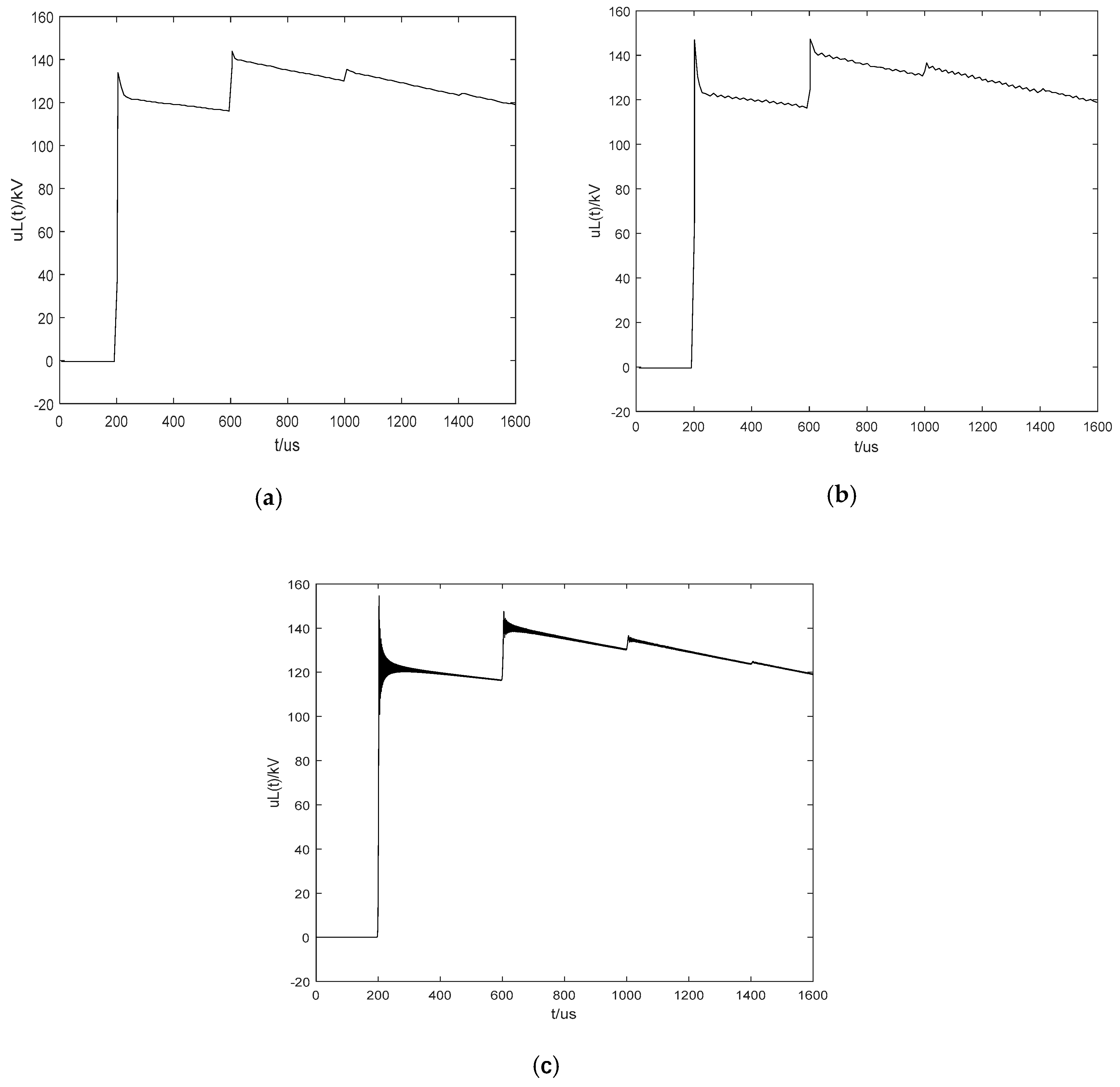The time integral step length of the PSM-BVM3, PSM-BVM2 and PSM-TR are $h_1=8.0\times {10}^{-8}\mathrm{s}$, $h_2=8.0\times {10}^{-8}\mathrm{s}$ and $h_3=1.0\times {10}^{-8}\mathrm{s}$, respectively. The calculation results of end terminal load voltage of nondestructive transmission line are shown in Figure 7, in which (a) is the result of the PSM-BVM3, (b) is the result of the PSM-BVM2 and (c) is the result of the PSM-TR.

It can be obtained from Figure 7 that the calculation results of steady state voltage of the three numerical methods are consistent, and the value is about 130 kV. The transient load voltage calculated by the PSM-BVM3 did not generate numerical oscillation due to the abrupt change of excitation signal, while for the PSM-BVM2 a little numerical oscillation appears in the calculation result and for the PSM-TR a large number of high frequency components are included in the calculation result. The reason is the time integral step of the PSM-BVM3 is large, and error accumulation can be well avoided, so numerical oscillation can be effectively avoided. Moreover, the time step of the PSM-BVM3 is larger than that of the PSM-TR, but the PSM-BVM3 is better than the PSM-TR in transient response of transmission line, which proves the improved effectiveness of the proposed coupled method.

The simulation results show that the proposed new method exhibits improved performance of faster decay rate to reduce the truncation error, which can effectively suppress the numerical oscillation phenomenon and reduce the transient calculation error of the transmission line caused by the oscillation. Besides, the proposed coupled method can compensate the drawback of the pseudospectral method which results in numerical instability caused by the singularity at the boundary and can also improve the calculation accuracy. Moreover, it can make improvements regarding the disadvantage of the boundary value method in which it is not easy to change the step size and the computational efficiency of which is not high. In conclusion, the method has the advantages of high computational precision, high computational efficiency, and numerical stability and is easy to expand in the practical application of transmission line problems in complex systems.

6. Conclusions

A Chebyshev pseudospectral–two-step three-order boundary value coupled method to resolve the transient response of transmission line is proposed in this study. In the given Chebyshev grid points, the telegraph equation is dispersed in space domain by the Chebyshev pseudospectral method, and the first-order linear differential equation is obtained. Moreover, such equation can be obtained by using the two-step three-order boundary value method to discrete the differential equation in the time domain. To avoid dimension disaster, the catch-up method of block tridiagonal is used to solve this equation. The numerical examples and simulation example prove that:

(1) The numerical results show that the coupled method in this paper is more accurate, efficient, and stable than the conventional PSM-DQM and PSM-BVM2 in the time domain. Moreover, the proposed coupled method is unconditionally stable in the time domain, and the spectral precision is convergent in the space domain. Furthermore, through the simulation of the lossless transmission line, it is proved that the proposed coupled method can better simulate the transient response of transmission line and can be applied in the practical application.

(2) The proposed coupled method exhibits improved performance of faster decay rate to reduce the truncation error, which can effectively suppress the numerical oscillation phenomenon and reduce the transient calculation error of the transmission line caused by the oscillation.

(3) The proposed coupled method can compensate the drawback of the pseudospectral method which results in numerical instability caused by the singularity at the boundary and can also improve the calculation accuracy. Moreover, it can improve on the disadvantage of the boundary value method, in which it is not easy to change the step size and the computational efficiency of which is not high.

Theoretical analysis and numerical simulation reveal that the proposed Chebyshev PSM-BVM3 has higher computation accuracy, efficiency, and better numerical stability. The coupled method is suitable for solving the transient response of the transmission line in the power system. Besides, applying the couple method, the issue of transmission oscillation and inaccurate signal transmission caused by delay, distortion, and crosstalk on the transmission line can be resolved. Furthermore, by employing the proposed method, the excitation signal in the power system can be accurately transmitted to the load. Therefore, the calculation benefit problem caused by the measurement inaccuracy can be improved, and the economic loss in the power system can be reduced.

Transient electromagnetic response on the transmission line can be coupled to the secondary and protection device, which will cause the secondary and protection device work abnormaly. Therefore, in order to accurately predict the electromagnetic transient process of transmission line, it is significant to analyze the transient response process of the transmission line. Thus, the proposed Chebyshev PSM-BVM3 method for transmission line transient response is significant in electromagnetic compatibility research.