Article

Parameter Estimation of Multi Frequency Hopping Signals Based on Space-Time-Frequency Distribution

College of Information and Communication Engineering, Harbin Engineering University, Harbin 150001, China
*
Author to whom correspondence should be addressed.
Symmetry 2019, 11(5), 648; https://doi.org/10.3390/sym11050648
Submission received: 13 April 2019 / Revised: 30 April 2019 / Accepted: 5 May 2019 / Published: 8 May 2019

Abstract

:
Frequency hopping spread spectrum (FHSS) communication is widely used in military and civil communication, and the parameter estimation of frequency hopping (HF) signals is of great significance. In order to estimate the parameters of multiple frequency hopping signals effectively, a blind parameter estimation algorithm based on space-time frequency analysis (STFA) and matrix joint diagonalization (JDM) is proposed. Firstly, the time domain signal received by the linear array is converted to the space-time frequency domain through the space-time frequency transformation, and the space-time frequency distribution (STFD) of the signal is obtained. Then the time-frequency point is extracted from the space-time frequency distribution map, the extraction of the hop is completed by the method of finding an “island”, and the space-time frequency matrix of each hop is constructed, and then the preliminary estimation of each jump frequency, jump time and jump period is completed. Finally, the space-time-frequency matrix of the same hop received by different array elements is jointly diagonalized by the matrix joint diagonalization algorithm, and the diagonalization matrix is obtained. On the basis of the diagonalization matrix, the root-MUSIC algorithm is used to complete the direction of arrival (DOA) estimation of the frequency hopping signal and the separation of the frequency hopping radio. The simulation results show that the proposed algorithm is effective in parameter estimation of multi-hopping signals. It can estimate the parameters of −4 dB signal-to-noise ratio (SNR). The accuracy rate of parameter (hop period, DOA, hop start time, hop end time, frequency hopping frequency set) estimation reaches 73.26%, and the sparse linear regression (SLR) algorithm reaches 70.15%. When the signal-to-noise ratio reaches 5 dB, the accuracy of estimation can reach 94.74%, and the SLR reach 85.64%. It has a good effect on parameter estimation of multi-hopping signals.

1. Introduction

Frequency hopping communication is a kind of spread spectrum communication, which is the main communication mode in the field of military communication, and has been widely used in military communication and civil communication [1]. Frequency hopping communication is widely used in the field of aerospace communication, such as Link16, and military satellites etc., because of its good confidentiality, strong anti-jamming ability, strong networking ability, anti-frequency selective fading, low requirements for channel phase frequency distortion characteristics, and easy compatibility with traditional communication systems [2,3]. Since frequency hopping communication has been used in the military, deployed for the purposes of interference and anti-interference, anti-sabotage and destruction has not stopped. In the actual communication, especially in short-wave band, the electromagnetic environment is very complex. Dense fixed-frequency signals, noise signals, external interference signals and various burst signals interweave with each other, which makes the detection of frequency-hopping signals very difficult, and also poses a severe challenge to communication investigation.
Frequency communication is the abbreviation of frequency hopping extended spectrum communication system, and the frequency hopping signal has a time-varying and pseudo-random carrier frequency [4]. It uses a binary pseudo-random code sequence to control the frequency of the output signal of the RF carrier oscillator, so that the carrier frequency of the transmitting signal jumps with the change of the pseudo-random code. Frequency hopping signal parameter recognition is of great significance; through it, the information of the enemy can be obtained by the military, so as to gain the first chance in warfare, and to design our own frequency hopping radio to prevent many kinds of interference and tracking by the enemies. Frequency hopping parameter identification also provides an important basis for signal demodulation and information acquisition. The frequency hopping parameters mainly include the frequency hopping rate, the frequent set and the frequency hopping width [5]. The frequency hopping sequence and frequency hopping DOA for frequency hopping radio sorting, in which the frequency hopping rate refers to the number of frequencies per second change, now frequency hopping communication is generally changed thousands of times per second. Frequency hopping refers to the frequency hopping set used in the frequency hopping communication system. Hopping bandwidth is the difference between the maximum and minimum frequency hopping. By estimating these parameters, the identification of frequency hopping signal and the sorting of frequency hopping radio can be completed, which lays a good foundation for the sorting of the frequency hopping signal in a communication reconnaissance system.
In addition to these signal physical parameters, signal wave direction (DOA) is also a very key parameter in frequency hopping communication reconnaissance, which plays an important supporting role in the task of sorting and signal recognition of FH network [6,7]. Because the carrier frequency of the hopping signal is not fixed, it changes randomly with time, so the DOA estimation method of a narrowband signal can’t be used directly for frequency hopping signal, which also brings some difficulties to the DOA estimation of frequency hopping signal. The frequency hopping signal is an instantaneous narrowband and macroscopic wideband signal.
At present, most of the detection and processing of frequency hopping signals focus on signal detection and parameter estimation in a time-frequency domain, but there are a few researches on the spatial information of frequency hopping signals. The mainstream method of time-frequency domain parameter estimation for frequency hopping signal is the time-frequency analysis method, as well as the compression perception and sparse Bayesian learning methods developed in recent years. The time-Frequency analysis method has a good processing ability for time-varying signals, which can’t be replaced by other methods, and the common time-frequency analysis is mainly divided into linear time-frequency analysis and quadratic time-frequency analysis. Linear time-frequency analysis mainly has a short-time Fourier transform [8], Gabor transformation and wavelet transform.Among them, discrete wavelet transform (DWT) is the most effective time-frequency analysis tool. The 1D and 2D DWT introduced in the literature [9] are often used for digital signal processing. Bilinear time-frequency representations include spectral graphs, Wigner-Wille distribution (WVD), pseudo-Wigner distribution (PWVD), smooth pseudo-Wigner distribution (SPWVD) [10,11,12], Margenau-Hill and so on. Chaos, entropy and fractals have drawn the interest of many researchers due to their mathematical modeling ability to solve a wide variety of real problems [13], and we can also use entropy theory and fractals for time-varying signal processing. Linear time-frequency transformation is easy to be affected by time-frequency resolution, and bilinear frequency distribution has a good time-frequency focus, but for multi-component signal, there is a serious time-frequency crossover [14,15,16], generating false signals. Because the received frequency hopping signal contains multiple components, it can’t be directly applied to the frequency hopping signal parameter identification. The spatial information of a frequency hopping signal, such as the direction of the wave, plays an important role in the sorting, signal tracking and interference of the network platform. The concept of space-time-frequency was first proposed in the literature [17,18], and the space-time frequency processing method was applied to blind source signal separation and DOA estimation, which achieved better performance than the traditional method. The paper [19,20,21] uses the space-time frequency method to carry on the direction finding and the signal separation to some non-stationary signals (such as linear FM, sound signal), but does not use the space time frequency to measure the frequency hopping signal direction. Multi-signal separation correlation research [2,22,23] has combined space-time frequency analysis with other algorithms including MUSIC, influence function, etc., used in DOA recognition, to achieve good results, but these algorithms are only applicable to narrowband signals, and not suitable for frequency hopping signals such as broadband signal, because of its terrible effect.
This article is mainly divided into five parts. The first part is the introduction of frequency hopping signal parameter estimation and is mainly concerned about frequency hopping signal jump frequent set rate, frequency hopping period, frequency hopping sequence, etc. Frequency hopping radio separation frequency hopping signal DOA is included too. The second part is the system model and frequency hopping parameters. Herein is introduced the frequency hopping signal model and linear array receiving model, and the construction of the space-time frequency matrix of each hop. The third part is parameter estimation of frequency hopping signal. It mainly introduces joint diagonalization algorithm of space-time-frequency matrix and root-MUSIC algorithm of frequency hopping DOA estimation to realize parameter estimation of multi-frequency hopping signal. In the fourth part, simulation experiments are designed to verify the effectiveness of the proposed algorithm. The last step is a summary of the proposed algorithm.

2. System Model and Frequency Hopping Parameters

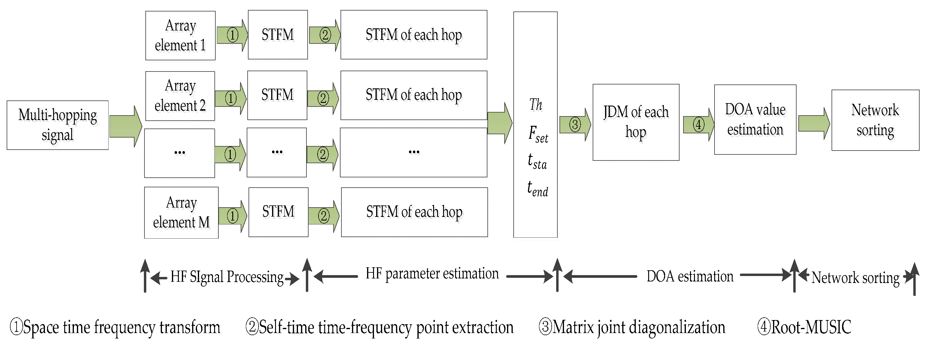
In this section, we mainly introduce the multi-component frequency hopping signal model, and the description of the signal acceptance by the linear array. We combined the time-frequency distribution to describe the space-time-frequency distribution transformation process. In this paper, a linear array is used to receive the frequency hopping signal, and then the time domain signals received by each array element are processed to complete the parameter estimation of the multi-hopping frequency signal and the sorting task of the frequency hopping radio station. The parameter estimation process in the paper is shown in Figure 1.
Firstly, the hybrid multi-frequency hopping signals received by each array element are subjected to space-time-frequency conversion to obtain a space-time-frequency matrix (STFM) containing all signal space-time-frequency information, and denoising processing is performed on the space-time-frequency domain. The algorithm of finding the island is used to estimate the number of hops and extract the time-frequency points of each hop. The STFM of each hop is constructed and the frequency hopping period (Th), frequency hopping frequency set ( F s e t ), start time ( t s t a ) and deadline ( t e n d ) of each hop are completed. Joint diagonalization the STFM of the same hop received by different array elements to obtain a joint diagonalization matrix (JDM), using this JDM to complete the DOA estimation of the frequency hopping signal, and using the DOA value to complete the frequency hopping radio sorting.

2.1. Frequency Hopping Signal Model

With the change of pseudo-random code, the frequency of hopping signal changes randomly, and the pseudo-random code sequence is used to control the carrier frequency sequence. The frequency hopping signal model in this paper as follows, assuming that there are N frequency hopping signals entering the receiver during the observation time Δ t , and the central frequency of the receiving machine is ω c , with the bandwidth Δ ω . Assuming the period of the nth frequency hopping signal s n ( t ) be T n , there are K hops in the observation time Δ t , and the carrier frequency and initial phase of the kth hop are f k and φ n k , then the expression of s n ( t ) as shown in Formula (1).
s n ( t ) = v n ( t ) k = 0 K 1 exp [ j ( 2 π f k t + φ n k ) ] r e c t ( t T n )
which t = t ( k 1 ) T n , v n ( t ) is the baseband envelope of the signal s n ( t ) , and rect represents a unit rectangular pulse.
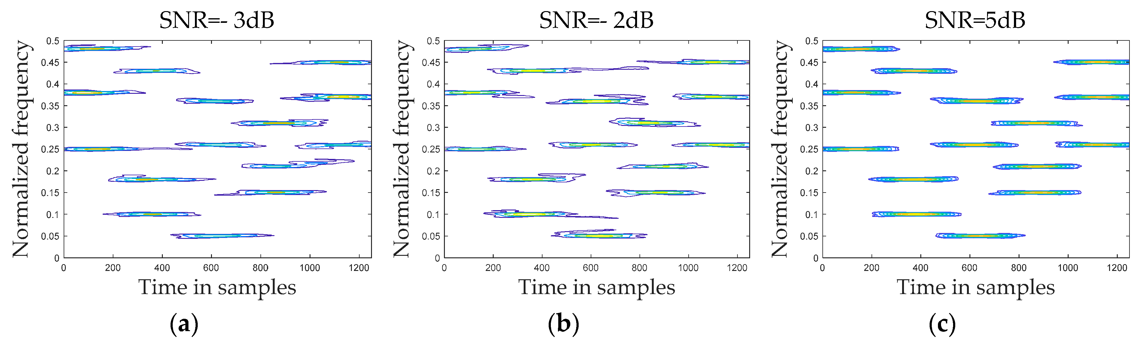
Actually, sampling frequency hopping signal is about 10 6   Hz , then sampling frequency obtained in this paper f s = 100 × 10 6   Hz , and Frequency hopping frequency in this paper is approximately f n , k = 25 × 10 6   Hz 
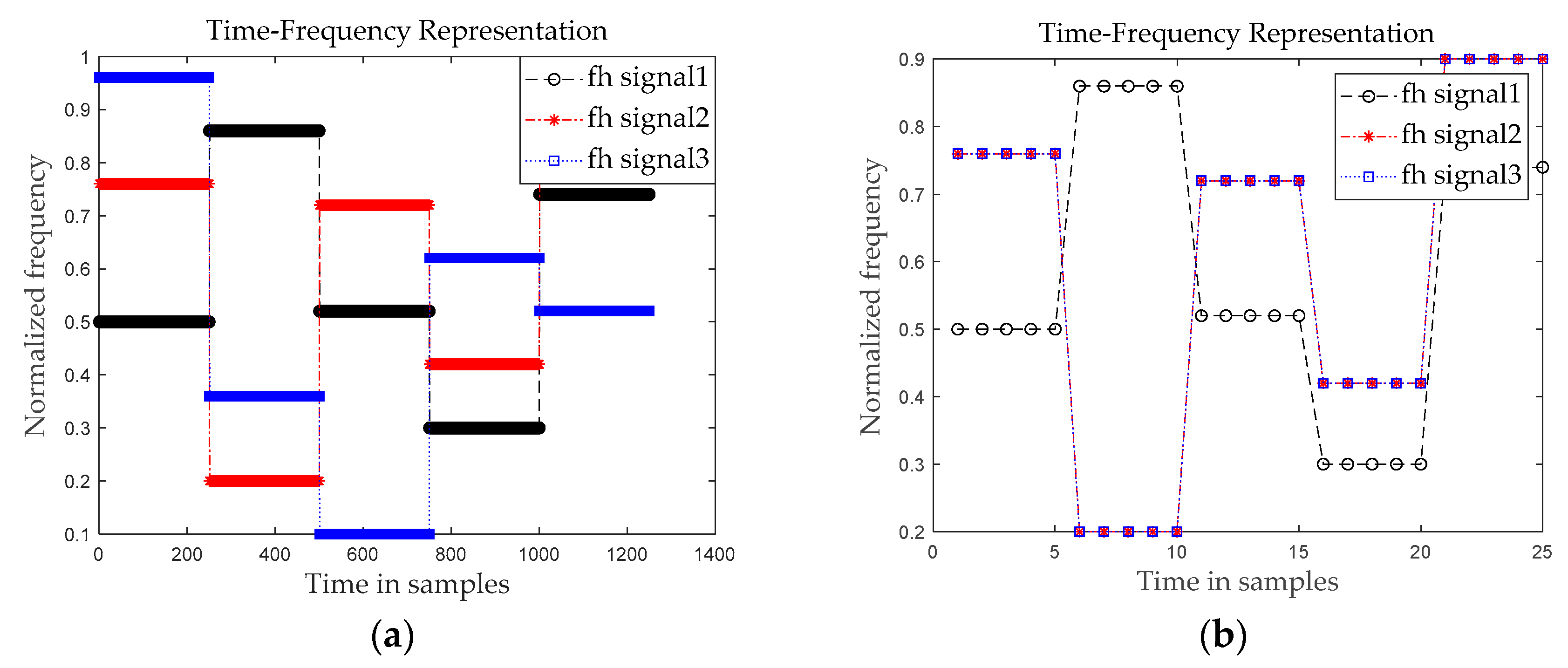
. The time-frequency diagram of the frequency hopping signal is shown in Figure 2. In order to normalize the frequency, the normalization formula f n , k = 2 f h , k f s is adopted, which is f n , k = 2 × 25 × 10 6 / 100 × 10 6 = 0.5   Hz . In this paper, the frequency hopping sequence is expressed as the Formula (2).
[ f 1 , f 2 , f 3 , f 4 , f 5 ] = [ f n 1 , f n 2 , f n 3 , f n 4 , f n 5 ] = [ 0.50 , 0.86 , 0.52 , 0.30 , 0.74 ]
in the upper formula, n = 1 , 2 , N represents the number of frequency hopping signals and k represents the kth hop of the nth signal.

2.2. Space-Time Frequency Distribution of Frequency Hopping Signal

The frequency of frequency hopping signal varies nonlinearly with time, which is a temporal signal and belongs to a typical non-stationary signal. The time-Frequency analysis method is the most common and effective method for analyzing time-varying signals. For example, the literature [22] uses time-frequency analysis and wavelet transform for medical time-varying signal processing, and achieved good results. Commonly used short-time Fourier transformations can be expressed as Formula (3).
σ ( t , f ) = x ( τ ) h * ( t τ ) e j 2 π f τ d τ
Commonly used QTFD can be expressed as Formula (4).
ρ x ( t , f ) = + G ( t , τ ) K x ( t , τ ) exp ( j 2 π f τ ) d τ
which G ( t , τ ) is the time delay kernel function. The QTFD possesses desirable properties such as local energy concentration IF, first moment visualization and reduced interference.
In this paper, a linear uniform array is used to receive the frequency hopping signal. Assuming that the array has an M array element, and the first array is located at the origin, and the spacing of each array is d ( d < λ m i n / 2 , λ m i n = c / f m a x ) , and θ n is the azimuth of each signal. The source is located in the far field, and the array noise is additive Gauss white noise. There is no correlation between the array elements, and the signal is not correlated with the noise. Thus, the array direction vector is expressed as Formula (5).
α ( θ ) = [ 1 , e j k i n d sin θ ,   , e j k i n ( M 1 ) d sin θ ] T
among them, k i n = 2 π / λ = ω i n / c , ω i n for signal carrier frequency. The time-domain signal received by the array is represented as Formula (6).
X ( t ) = Y ( t ) + N ( t ) = A S ( t ) + N ( t )
which X ( t ) = [ x 1 ( t ) , x 2 ( t ) , x M ( t ) ] T , S ( t ) = [ s 1 ( t ) , s 2 ( t ) , s M ( t ) ] T , N ( t ) = [ n 1 ( t ) , n 2 ( t ) , n M ( t ) ] T , M represents the number of array elements, and N representing the number of frequency hopping signals.
Through (5) Formula, we can see that the array direction vector and manifold matrix are related to the carrier frequency ω i n and jump with the frequency hopping of the carrier, when the carrier frequency changes, corresponding to the array direction of the vector changes also occur. Frequency hopping communication carrier frequency has been changed; it can’t be fixed directly to the fixed-frequency signal processing method applied to the frequency hopping communication. We know that the frequency of FH communication is fixed in a hop duration, that is, the direction vector of the array is unchanged during this hop duration, and it can be used as narrowband signal processing. Based on this, the frequency hopping signal can be decomposed into one hop, so that the analysis object can be simplified to a narrowband model.
Frequency hopping signals received by antenna arrays contain abundant spatial information in the direction matrix. The space-time-frequency analysis used in this paper is to extend the research object of traditional space-time processing to time-frequency domain, that is, to analyze the signal in time-frequency domain first, then to select effective time-frequency points in time-frequency domain, and to use these time-frequency data to form space-time-frequency matrix. The benefits of STFD over the spatial correlation matrix in a nonstationary signal environment is the direct exploitation of the information [24,25]. We first review the definition and basic properties of the STFDs. STFDs based on Cohen’s class of TFD were introduced in [17], and its applications to direction finding and blind source separation have been discussed in [25,26,27].
The discrete form of the smoothed pseudo Wegener Ville distribution can be expressed as Formula (7).
D x x ( t , f ) = t = + l = + φ ( l , τ ) x ( t + l + τ ) x * ( t + l τ ) e 4 j π f τ
where * indicates complex conjugate, the space-time-frequency distribution is to process the snapshot vectors X ( t ) received by the array. The space-time-frequency distribution matrix is defined as Formula (8).
D X X ( t , f ) = t = + l = + φ ( l , τ ) X ( t + l + τ ) X * ( t + l τ ) e 4 j π f τ
to bring (6) into Formula (8).
D X X ( t , f ) = D X X ( t , f ) + 2 R e [ D N Y ( t , f ) ] + D N N ( t , f )
the noise is zero mean Gaussian white noise and is not related to the signal. To expect (9) form, then E [ D Y N ( t , f ) ] = E [ D N Y ( t , f ) ] = 0 , Then Formula (9) is as Formula (10).
E [ D X X ( t , f ) ] = D Y Y ( t , f ) + E [ D N N ( t , f ) ] = A D S S ( t , f ) A H + σ 2 I

2.3. Frequency Hopping Hop Extraction and Space Time Frequency Matrix Construction

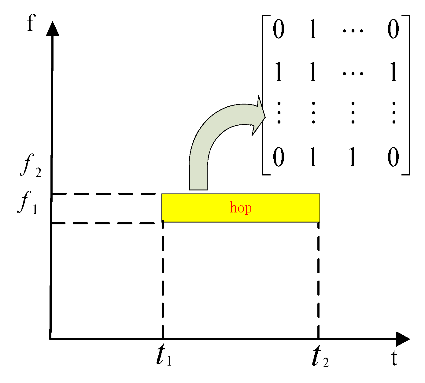
On the basis of the space-time frequency distribution graph obtained in the previous section, this section mainly completes the time-frequency point extraction and the space-time frequency matrix construction of each hop. Since the space-time frequency values are plural, it is not convenient to find the self-item frequency point of each hop directly on the space-time frequency distribution map, so this paper first converts all values to 0 and 1 by threshold, and then finds a position on the space time-frequency distribution that contains only 0, 1, and the value corresponding to the position of 1 is the value of the time-frequency point.
(a) Construct 0, 1 space-time frequency distribution matrix.
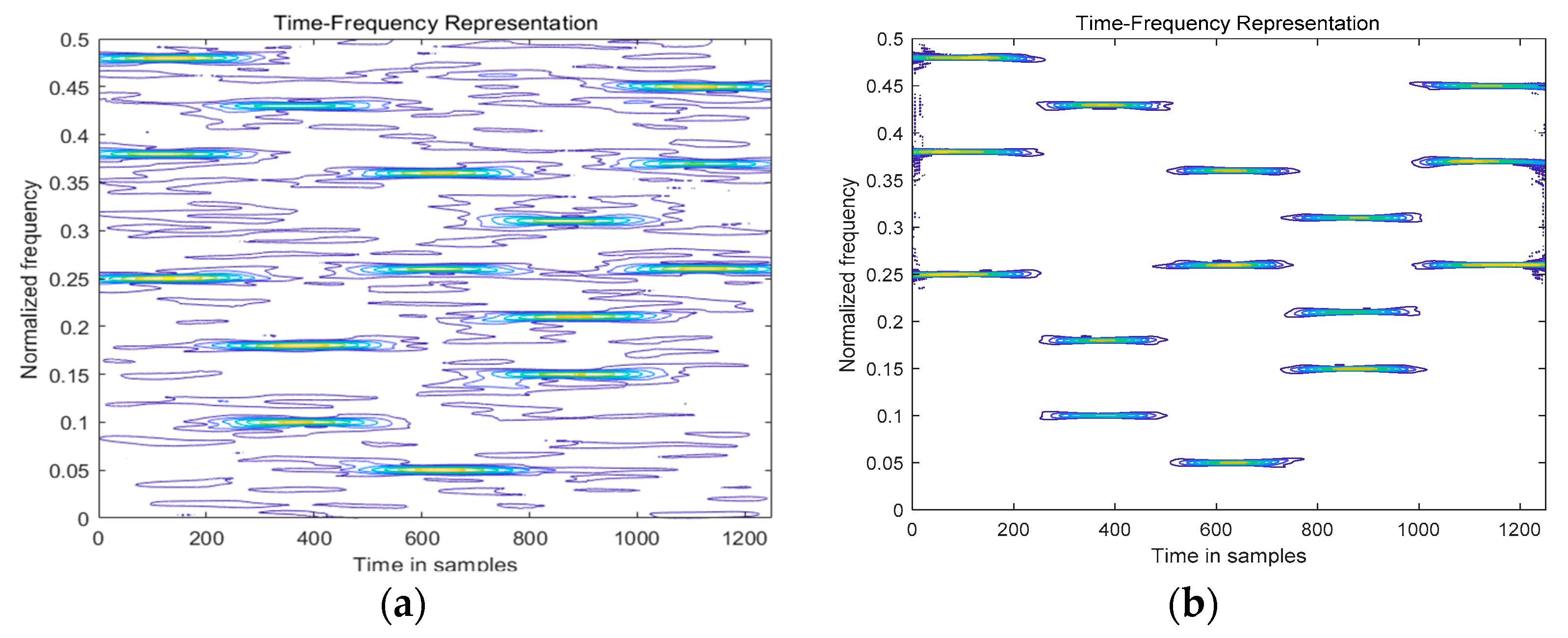
Step1: The array receiving signal is made of linear space-time frequency transformation and bilinear space-time frequency transformation to obtain S T F T X 1 X 1 ( t , f ) and S P W V D X 1 X 1 ( t , f ) as shown in Figure 3 and Figure 4, which do point multiplication, and the space-time frequency combination Matrix S T F C X 1 X 1 ( t , f ) is obtained, S T F T X 1 X 1 ( t , f ) = S T F T X 1 X 1 ( t , f ) S P W V D X 1 X 1 ( t , f ) , and the “ ” is Hadamard product.
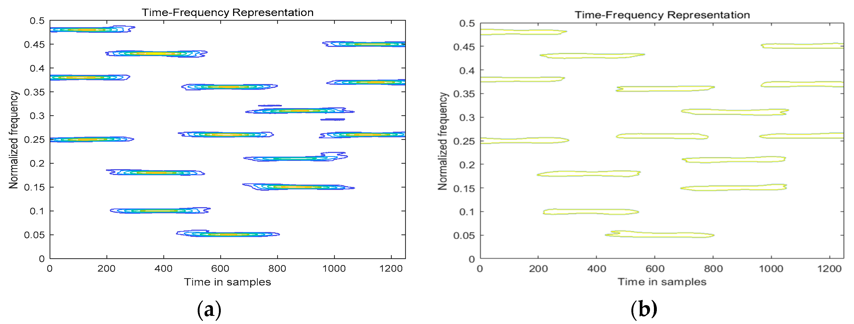
Step2: The S T F C X 1 X 1 ( t , f ) is truncated to get the self-time frequency graph T F A X 1 X 1 ( t , f ) as Formula (11).
T F A X 1 X 1 ( t , f ) = { 1 , | S T F C X 1 X 1 ( t , f ) | T h 0 , | S T F C X 1 X 1 ( t , f ) | < T h
which T h is Cut-off threshold and T h = μ Mean { a b s [ S T F C X 1 X 1 ( t , f ) ] } , the μ is threshold factor. Through the above operation, a matrix T F A X 1 X 1 ( t , f ) containing only 0 and 1 elements is obtained.
(b) Self time and frequency point extraction.
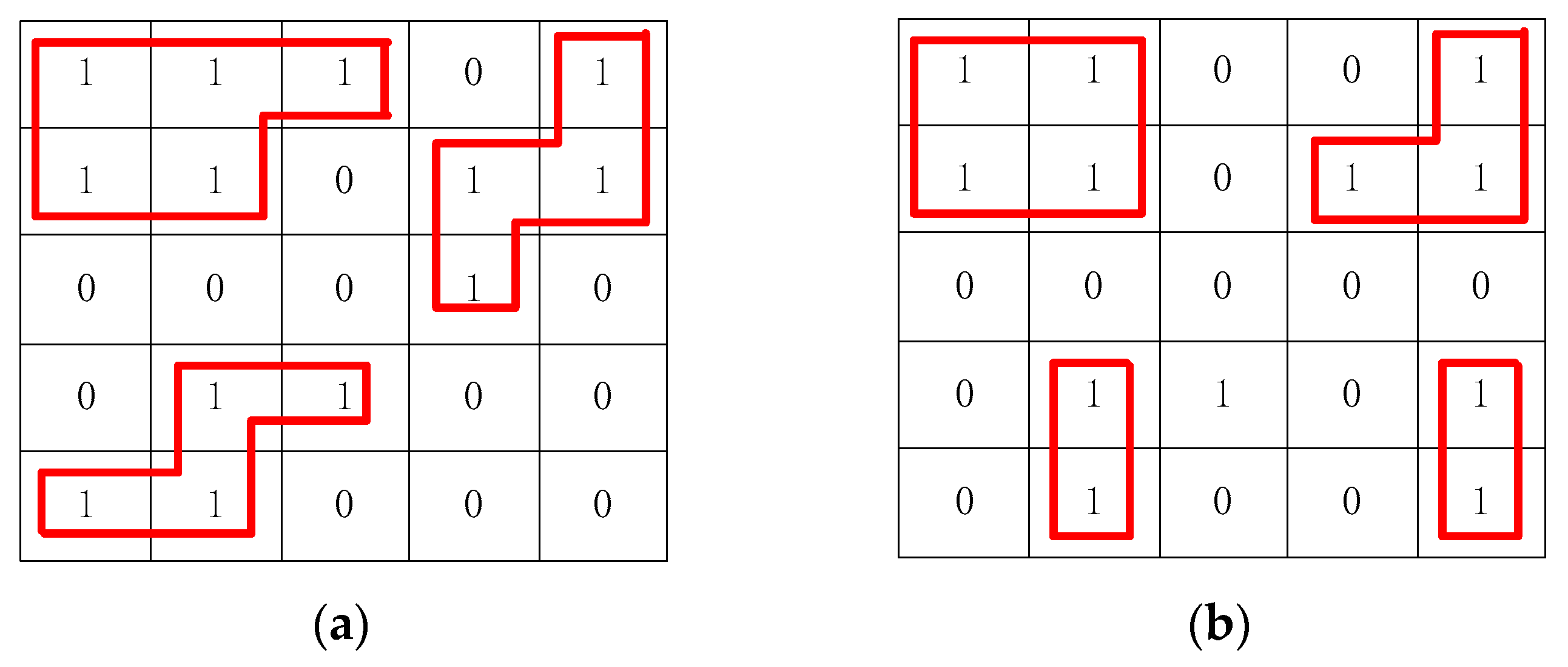
Each hop is extracted on the space-time frequency graph, and its corresponding time-frequency value is formed to form the space-time frequency matrix of each hop. In this paper, we use the method of finding “islands” to traverse the T F A X 1 X 1 ( t , f ) obtained by Formula (11) and find out the number N of all “islands” in the space-time-frequency matrix. As shown in the 
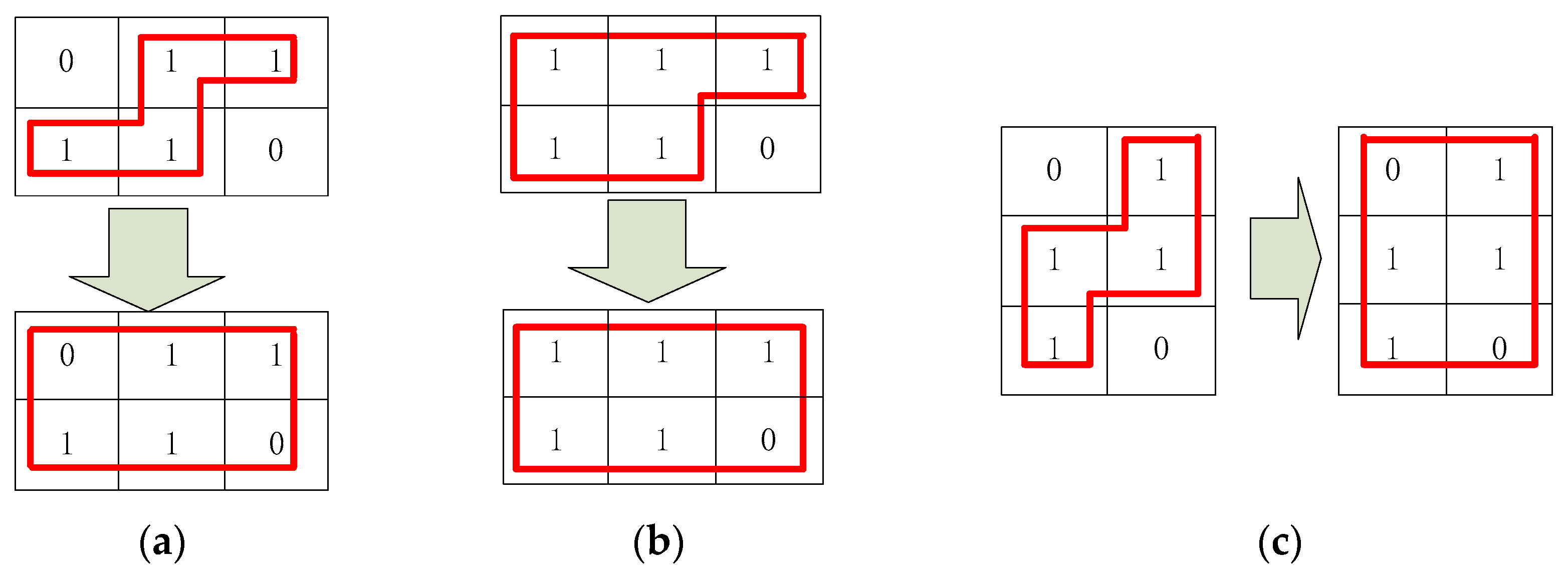
Figure 5, in a matrix, surrounded by red rectangular frames is called “islands”, and the number of islands is the number of hops. The observation found that there are three islands in the Figure 5, a total of four islands in the right image, that is, three hops on the left and four hops on the right.
Each of these “island” corresponds to a hop in the frequency hopping signal, only need to find the islands in the matrix, you can extract the time frequency point of each hop from the space-time frequency matrix, these self-entry time frequency points to form the hop’s space-time frequency matrix. The matrix obtained by the Formula (11) is “C” that contains only two elements of 0,1 and traverses the matrix. The interconnected element 1 is called an island, and find all the islands in the matrix. The total number of islands is recorded K h o p , and the coordinates of the element 1 in each island are recorded. If the Element 1 in the island h o p 1 is taken as the location of the element. The coordinates of the hop self-term time point can be expressed as Formula (12).
i n d h o p 1 = { ( x 1 , y 1 ) , ( x 2 , y 2 ) , ( x n , y n ) | ( x n , y n ) C }
Finding 1 of each island in Matrix C, recording its position in the form of an island. According to this method, the location of 1 in all islands is found, and the time-frequency points of self-term are extracted.
The space-time frequency matrix obtained after the (11) transformation is recorded as P , according to the coordinate value of each island obtained by Formula (12), the corresponding position is found in Matrix P k , the space-time frequency value of the corresponding position is taken out, and the space time frequency value in the same block is recorded as Y according to the principle that the corresponding position remains unchanged. Each space-time frequency matrix corresponds to a hop, then all hops corresponding to the space-time frequency matrix are recorded as { P 1 , P 2 , P L | L = K h o p } .
The position composition of the self-term time-frequency points extracted from each island may not be a rectangular shape. At this time, it needs to be adjusted accordingly. Without destroying the whole structure, the corresponding position is complemented by 0, so that each hop constitutes a matrix. There are three hops in the left graph of the Figure 4. They are hop1, hop2 and hop3 from left to right and from top to bottom. By doing the following transformation, the space-time-frequency values of all hops can be changed into the space-time-frequency matrix shown in the Figure 6.

3. Frequency Hopping Signal Parameter Estimation

This part is mainly based on the space-time frequency matrix of each hop extracted in the second part to estimate the frequency hopping parameters. The first section is the basic parameter estimation of the frequency hopping signal, including the frequency hopping frequency sets, hopping period, jump time, etc. the second section of the frequency hopping signal DOA estimation. Firstly, the matrix joint diagonalization algorithm based on the minimum mean square error is used to diagonalize the space-time-frequency matrix of the same hop received by different array elements, and a joint diagonalization matrix is obtained. Then the root-MUSIC algorithm is used to complete the DOA estimation of each hop. Finally, the DOA values of all hop estimates are clustering according to the clustering algorithm.

3.1. Hopping Basic Parameter Estimation

This section mainly estimates the parameters based on the coordinates of the elements in the space-time frequency matrix of each hop obtained in the original space-time frequency matrix, where it is assumed that the sampling frequency F s of the signal is known, and when the scale value of each hop self-entry frequency point along the timeline and frequency axis on the space-time frequency graph is found. The scale values of each hop on the space-time frequency axis can be obtained by averaging the parameters corresponding to the same hop in different arrays.
The time t in Figure 7 is replaced by a number of points. For this hop, Th can expressed as Formula (13).
T m k [ n ] = ( t 2 t 1 ) / F s
where [ n ] denotes the nth signal, m denotes the m-th element, and K denotes the kth hop of the frequency hopping signal, and the start time of the frequency hopping signal t m k [ k ] = t 1 / F s , and the cutoff time for the hop is t m k [ k ] = t 2 / F s , and The carrier frequency of the hop can be expressed as Formula (14).
F m k [ n ] = 2 × ( f 2 f 1 ) × F s
Then the carrier frequency of the k-th hop of the n-th FH signal can be expressed as F k [ n ] = m e a n { F 1 k [ n ] , F 2 k [ n ] , , F M k [ n ] } , The starting time of the K hop of the nth frequency hopping signal is expressed as t k [ n ] = m e a n { t 1 k [ n ] , t 2 k [ n ] , , t M k [ n ] } . The deadline is expressed as t k [ n ] = m e a n { t 1 k [ n ] , t 2 k [ n ] , , t M k [ n ] } , The frequency hopping period T n of the nth frequency hopping signal is expressed as Formula (15).
T n = m e a n { T m 1 [ n ] , T m 2 [ n ] , , T m k [ n ] }
The jump frequency rate F n is expressed as F n = 1 / T n .

3.2. Joint Diagonalization of Space-Time-Frequency Matrix Based on Minimum Mean Square Error

Matrix joint diagonalization was first proposed mainly for signal blind separation (BSS) and independent component analysis (ICA) [28]. Joint diagonalization is mainly to find a diagonal matrix to replace a matrix set, which contains many sub-matrices. Mathematical formulas can be expressed as: Assuming that set γ contains K matrix A 1 , A 2 , , A k C N × N , joint diagonalization is to find a diagonal matrix B C N × N and K related diagonal matrix 1 , 2 , , k C N × N to make C L S achieve the minimum value as Formula (16).
C L S ( v , 1 , 2 , , k ) = k = 1 K ω k | | k v k v H | | 2
Considering that the multiple hops of the same frequency hopping signal received by each array element, many space-time frequency matrices are obtained, and the information of each space-time frequency matrix cannot be synthesized separately. In this paper, the joint diagonalization algorithm based on the minimum mean square error is used to estimate the parameter of frequency hopping signal. If there are M elements { P 1 , P 2 , , P M } in an array, and the received signal of p 1 element is expressed as { h o p 1 ( 1 ) , h o p 2 ( 1 ) , , h o p K ( 1 ) } after space-time-frequency transformation, then the received signal of P M element is expressed as { h o p 1 ( M ) , h o p 2 ( M ) , , h o p K ( M ) } , where h o p K ( M ) is the k-th hop space-time-frequency matrix of the frequency hopping signal received by the first element of K. If the same hop received by different elements is recorded as a set of γ i , γ i expressed as Formula (17).
γ i = { h o p 1 ( 1 ) , h o p 1 ( 2 ) , , h o p 1 ( M ) }
Then γ N is γ N = { h o p N ( 1 ) , h o p N ( 2 ) , , h o p N ( M ) } , so that the space-time-frequency matrix of the same hop received by different elements can be formed into a set. Then a diagonal matrix v is found according to the principle of minimum mean square error, and the set of hop space-time-frequency matrices is represented by the diagonal matrix v . In order to find the diagonal matrix v , making the Formula (16) the smallest, it is mainly divided into the following two steps:
Step1: Change the diagonal matrix v and take the target matrix v as the variable. First initialize a diagonal matrix v of the same size as the h o p N ( M ) , assuming that the size of v is N R × N C , then v is represented as a column v = [ v 1 , v 2 , , v N c ] , and (16) the formula can be expressed as Formula (18).
C L S ( v , 1 , 2 , , k ) = k = 1 K ω k | | k v k v H | | F 2 = k = 1 K ω k | | k n = 1 N c λ n [ k ] v n v n H | | F 2
where λ n [ k ] is the element at the coordinate position (n, n) of the diagonal matrix k , * H representing conjugate transposition, recorded as A ˜ k = A k n = 1 n l N c λ n [ k ] v n v n H , then Formula (18) can be expressed as Formula (19).
C L S ( v , 1 , 2 , , k ) = k = 1 K ω k | | A ˜ k λ l [ k ] v l v l H | | F 2 = i = 1 n ω k T r { [ A ˜ k λ l [ k ] v l v l H ] H [ A ˜ k λ l [ k ] v l v l H ] } = C ˜ T r { k = 1 K ω k λ l [ k ] [ A ˜ k H v l v l H + v l v l H A ˜ k H ] } + T r { k = 1 K ω k ( λ l [ k ] ) 2 v l v l H v l v l H } = C ˜ v l H [ i = 1 n ω k λ l [ k ] [ A ˜ k H + A ˜ k ] ] v l + ( v l H v l ) 2 k = 1 K ω k ( λ l [ k ] ) 2
where T r { · } denotes the trace of matrix, we can find that C ˜ is a constant value and the value of C ˜ is independent of v l . If v l is expressed as v l = b β , where b is a real number greater than 0, β is a unit normal vector and β β H = 1 , the expression can be expressed as Formula (20).
C L S ( b , β ) = C ˜ 2 b 2 β H P β + b 4 p
where p = k = 1 K ω k ( λ l [ k ] ) 2 is a constant and P = k = 1 K ω k λ l [ k ] A ˜ k is a square matrix of N × N size, the Formula (20) is equal to zero. If we derive b, we can get b = 0 or b 2 = 1 p β H P β and replace it with Formula (20), because β H β = 1 , then
C L S ( β ) = C ˜ β H P 2 β
we can know that when β is the eigenvector corresponding to the largest eigenvalue of P , the above Formula (21) achieves the minimum.
Step2: With diagonal matrix 1 , 2 , , k as a variable, the corresponding k is updated when the minimum value of Formula (18) is obtained. Formula (18) is decomposed into K independent linear minimization problems as Formula (22).
C k ( k ) = | | A k v k v H | | F 2
Here we do the following transformation: making the parameter vector is λ k = d i a g { k } , and the A k columns are stitched together a = vec { A k } ( vec is a column mosaic function), then the formula can be reduced to a linear minimization problem as Formula (23).
C k ( k ) = [ a H λ k ] H [ a H λ k ]
where H is defined as H = ( v * L ) ( L v ) , L is N × 1 the unit vector, then the linear minimization problem is transformed into the Formula (24).
λ k = [ H H H ] 1 H H a
Through the above operation, the Formula (16) obtains the minimum value, then replacing the original k with λ k and alternating the operation between the two Steps (1) and (2), when the minimum mean square error C L S satisfies a certain threshold condition, and the matrix v at this time is the space-time frequency combined diagonalization matrix of the asked hop.

3.3. FH Signal DOA Estimation

This section is based on each hop joint diagonalization matrix obtained in the previous section, using the spatial information it contains to complete the wave direction (DOA) estimation of each hop. Because the expansion subspace by the signal feature vector is consistent with the expansion subspace by the array guide vector, and according to the orthogonality of the signal subspace and the noise subspace, the MUSIC algorithm can be used for DOA estimation of the joint diagonalization matrix. Because the MUSIC algorithm needs spectral peak search, the complexity is high. In this paper the root-MUSIC algorithm, which does not need spectral peak search, is used to estimate the DOA of the hop, and the root MUSIC algorithm is a polynomial root finding form of the MUSIC algorithm. The time-frequency MUSIC space spectrum of the signal can be obtained by replacing the covariance matrix in the traditional algorithm with the modified space-time frequency matrix. Thus, the DOA estimation of the signal is obtained. Define a polynomial as Formula (25).
p l ( z ) = u l H p ( z ) , l = K + 1 , , M
where u l is the lth eigenvector of matrix R, and in order to extract information from all noise eigenvectors at the same time, we hope to find the zero point of MUSIC. Because the former is also a polynomial of z, there exists a power term of z * . Because only interested in the z value on the unit circle and replaced p T ( z 1 ) by p H ( z ) , the polynomial of root MUSIC is obtained as Formula (26).
p ( z ) = z M 1 p T z 1 U N U N H p ( z )
where p ( z ) is the 2 ( M 1 ) quadratic polynomial, when its root and unit circle are mirrored, the phase of the K roots z ^ 1 , z ^ 2 , , z ^ K with the maximum amplitude in the unit circle is given to estimate the direction of the wave, θ ^ m can be expressed as Formula (27).
θ ^ m = a r c s i n [ λ 2 π d a r g ( z ^ m ) ] , m = 1 , 2 , K
the DOA estimate obtained by each hop is expressed as { θ h o p 1 , θ h o p 2 , , θ h o p N } .

3.4. Frequency Hopping Network Table Sorting

In this subsection, on the basis of the DOA estimation of each hop obtained in the previous section, the K-means clustering algorithm is used to identify the number of frequency hopping signals and sort the frequency hopping radio. The paper’s main research focus is synchronous networking radio, which changes the carrier frequency at the same time with each station in the network, and the hop time is basically the same, so a hop can be divided into several networks according to DOA parameters. The traditional K-means algorithm is completely random for K initial centroids, which results in slow convergence. The k-means++ algorithm is used to optimize the method of K-means random initial centroids, which is divided into two steps: K value determination and DOA estimation clustering.
Step1: The K value of clustering center is determined by contour coefficient method. The contour coefficient combines the condensation degree and the separation degree of the cluster, which is determined by the cluster non-similarity a i and the non-similarity b i between the clusters, as Formula (28).
s ( i ) = b ( i ) a ( i ) m a x { a ( i ) , b ( i ) }
the mean value of s ( i ) for all samples is called the contour coefficient. By enumerating, the K is from 2 to a fixed value, repeatedly running several times on each K value (avoiding the local optimal solution), and calculating the average contour coefficient of the current k, and finally selecting K corresponding to the value of the maximum contour coefficient as the final number of clusters.
Step2: K-means++ algorithm is used to complete DOA clustering. By randomly selecting the first clustering center μ 1 and calculating D ( x i ) = arg m i n | | x i μ r | | 2 2 , the algorithm chooses K maximum values and finds the corresponding clustering center, which is the number of frequency hopping signals, and the corresponding hop of DOA clustered to the same clustering center is the frequency hopping signal of the same network. In combination with Section 3.1, the frequency hopping set of the frequency hopping signal, the frequency hopping sequence of the frequency hopping signal and the frequency hopping time can be estimated, and the parameters of the frequency hopping signal can be estimated.

4. Simulation Experiment

This part is mainly to verify the algorithm proposed in the paper and design three simulation experiments. The first part of this section gives the multi-hopping signal simulation parameters and evaluation indicators. The second part of the verification shows the effectiveness of the proposed finding “island” algorithm for hop and self-space- time-frequency point extraction. The third part verifies the accuracy of the estimation of multi-hopping parameters by the algorithm proposed in the paper. The last part verifies the robustness of the proposed algorithm. The details are as follows.

4.1. Simulation Environment and Parameter Design

In order to verify the effectiveness of the proposed algorithm, different frequency hopping signals are generated by setting different parameters. In the experiment, the frequency hopping station adopts the synchronous orthogonal networking mode, so that each orthogonal network station in the same network has a unified time reference, and each station in the network has the same carrier frequency hopping time, frequency hopping period and frequency hopping rate. In the experiment, orthogonal hopping sequences are designed so that the frequency does not collide or there are few collisions during communication. The experimental setup sets the multi-hopping signal reception in the linear array under the underdetermined condition (i.e., the number of elements is less than the number of signals). The detailed frequency hopping signal parameters are set as follows. The linear array designed in the experiment contains two array elements, the first array element is located at the origin position; a total of three frequency hopping signals are included, and the DOA angle of the three frequency hopping signals are 10 ° , 20 ° , 70 ° .
The specific parameter settings are shown in Table 1. The sampling frequency (Fs), observation duration (t), the hop period (Th), where the corresponding sampling points are used instead of the Th, the frequency hopping frequency set ( f h , k ). A total of three sets of frequency hopping signals are set here, Group1, Group2 and Group3, each group contains three frequency hopping network stations. For example, the frequency hopping signals sent by three frequency hopping network stations in Group1 are F h 11 , F h 12 ,   F h 13 . The Fs is uniformly set to 100 MHz. Each frequency hopping signal in the first group contains 5 complete hops with a hop period of 250. The second set of frequency hopping signals F h 21 contains 3 complete hops, where Th is 250 and the observation time is 12.5 microseconds; F h 22 contains 4 complete hops and F h 23 contains three complete hops. The third group of frequency hopping signals has a duration of five microseconds and a hop period of 100. Each network station transmits a frequency hopping signal containing five complete hops.
The performance of frequency hopping estimation is measured by RMSE. Frequency hopping estimation error is defined as Formula (29).
R M S E f = 1 N K U n = 1 N k = 1 K u = 1 U ( f n k ( u ) f ^ n k ( u ) ) 2
where f ^ n k ( u ) is the estimate of the frequency, f n k ( u ) is the true value of the frequency, and n represents the nth frequency hopping signal, and K represents the K-th hop of the nth Signal, where U represents a total of one U random test, and the frequency estimation error definition is similar, the mean square error of the jump cycle estimation is defined as follows Formula (30).
R M S E T h = 1 T h 1 N U n = 1 N u = 1 U ( T n ( u ) T ^ n ( u ) ) 2
The DOA estimation error of frequency hopping signal is defined as follows Formula (31).
R M S E θ = 1 N U n = 1 N u = 1 U ( θ n ( u ) θ ^ n ( u ) ) 2

4.2. Feasibility Experiment Verification

This part mainly verifies the feasibility of the finding “island” algorithm for multi-hopping signal hop estimation and self-space time-frequency point extraction. In the proposed algorithm, the correct estimation of the number of hops is of great significance for the estimation of multi-hopping parameters. The experiment verifies the mixed signal composed of the three frequency hopping signals transmitted by the three frequency hopping stations of the synchronous orthogonal network. The specific parameters are shown in Group1 and Group2 in the above Table 1, and the sampling frequency is 100 MHz.
It can be found from the above Table 2 that when the signal-to-noise ratio is −10 dB, there are 15 hops in the multi-hopping signal, and the number of hops estimated by the algorithm in the text is 30. By performing multiple Monte Carlo experiments, the number of Hops is estimated correctly 30.42%. when the signal-to-noise ratio is −3 dB, the correct rate is 95.56%, and the estimation effect is better; when the signal-to-noise ratio reaches 5 dB, the correct rate reaches 100%; when the signal-to-noise ratio is lower than −3 dB, the signal’s time-frequency point is submerged by noise, which has a great influence on the estimation of the number of hops.
It also verifies the validity of the finding “island” algorithm for the extraction of self-term time-frequency points. Using the “island” algorithm, the hop number estimation of the multi-hopping signal is first completed, and then the time-frequency points of each hop are extracted to form a space-time-frequency matrix. For different signal-to-noise ratios, the effectiveness of the algorithm for the time-frequency point extraction of the self-term time-frequency point is verified by the algorithm with signal-to-noise ratio of −3 dB, −2 dB and 5 dB. The experimental results are shown in Figure 8.
By observing Figure 8, it can be found that when the signal-to-noise ratio is −3 dB, the time-frequency points of all hops can be extracted, but the extracted time-frequency points contain a lot of noise, which makes the space-time-frequency diagram unsmooth and has many burrs; When the signal-to-noise ratio is 5 dB, it can be found that the extracted time-frequency points are relatively pure, and the space-time-frequency diagram is smooth and does not contain noise. Therefore, the finding “island” algorithm is used to extract the time-frequency points of the self-term. The effect is better when the signal to noise ratio is greater than −3 dB.

4.3. Estimated Accuracy Experiment

In this part of the experiment, the relationship between the accuracy of parameter estimation and the signal-to-noise ratio of multi-component frequency hopping signals based on space-time-frequency distribution is verified. The experimental signal-to-noise ratio ranges from −4 dB to 20 dB, and the step size is 2 dB. The three mixed signals transmitted by the three frequency hopping stations of the synchronous orthogonal network are used for parameter estimation. Specific parameters on the Table 1 Group1. In order to verify the validity of the proposed algorithm for multi-hopping signal parameters estimation, and compared with the multi-hopping parameter estimation algorithm based on Sparse Linear Regression (SLR) proposed in the reference [29,30]. The accuracy of each parameter estimation is shown in Figure 9.
As shown in the above Figure 9, the multi-hopping signal parameter estimation algorithm based on space-time-frequency distribution and the sparse linear regression method are compared, and the frequency hopping period, frequency hopping frequency set, frequency hop start time and end time estimation are completed. As shown in Figure 9a, when the signal-to-noise ratio is lower than 0dB, the error of the hopping period estimation is more than 50%, and the estimation error is large. It can be seen from the figure that the signal-to-noise ratio is between −2 dB and 12 dB. At the time, the accuracy of the algorithm proposed in the paper is significantly better than that of the SLR method. When the SNR is greater than or equal to 18 dB, the estimation accuracy reaches 100%. Figure 9b shows the DOA estimation curve of the frequency hopping signal. It can be seen that when the SNR is lower than 0 dB, the DOA angle is larger, the estimation error is smaller, and when the SNR is greater than 0 dB, the gap gradually disappears. When SNR = 5 dB, the DOA estimation error is 5 ° . Figure 9c is the estimated error map of the frequency hopping frequency set. When the SNR is small, the error of the frequency hopping frequency estimation is large due to the error of the time-frequency point extraction. It can be seen that when the SNR is greater than 5 dB, the extraction of the time-frequency point of the self-term can obtain a clear space-time-frequency diagram, and the estimation error of the frequency hopping frequency decreases. It can be seen that when the SNR is greater than 10 dB, the estimation error falls within several hundred Hz. Figure 9e,f is the estimated error graph of the start time and end time of the frequency hopping signal Hop. When the SNR is less than 0 dB, the proposed algorithm error is larger than the SLR algorithm. As the SNR increases, the SNR is greater than 6 dB, the algorithm proposed in the paper works well. When SNR = 6 dB, the estimated accuracy can reach 100%. Figure 9d is the result of the hopping network station sorting result. When SNR = 5 dB, we can find that the clustering gets three cluster centers, so there are three frequency hopping stations. Based on the above analysis, the proposed algorithm is better than the SLR algorithm when the SNR is greater than 0 dB.

4.4. Robust Experiment

The number of sampling points selected in the paper is 1250, and the number of sampling points per hop is 250. If the number of sampling points is small, is the parameter estimation effect of the proposed algorithm still valid? In order to verify the robustness of the proposed algorithm, this part of the experiment was designed. Here, the frequency hopping signals of Group1 and Group3 in the Table 1 are selected. The sampling points are 500~1250, and the step size is 75, that is, the number of points per hop is 100~250. Here, we mainly verify the variation of the estimation error of the frequency hopping period and the frequency hopping frequency with the number of sampling points per hop under different SNRs when each hop is 20 to 250 points. The experimental results are shown in Figure 10.
From the Figure 10a, it can be found that when the number of data points sampled per hop is from 100 points to 250 points, the accuracy of the frequency hopping period estimation is small under the same SNR, and when the number of sampling points is the same, When the signal-to-noise ratio is different, the signal-to-noise ratio is larger, and the accuracy of the frequency hopping period estimation is higher. Similarly, as shown in Figure 10b, when the SNR are 5 dB and 10 dB, the frequency hopping frequency estimation accuracy is basically not change. It can be illustrated by these two graphs that the proposed algorithm has better robustness and less influence by the number of sampling points.

4.5. Discussion

Through the simulation experiments designed in Section 4.2, Section 4.3 and Section 4.4, we can find the parameter estimation algorithm of the multi-hopping signal based on space-time-frequency distribution and the frequency hopping signal parameters of the stations transmitted by the synchronous orthogonal network. The frequency hopping station has a better sorting effect. Compared with the base and SLR algorithms proposed in the literature, the algorithm has a small amount of computation. When the SNR is greater than 0 dB, the proposed algorithm is significantly better than the SLR algorithm. However, the algorithm proposed in the paper also has shortcomings. First, the correct estimation of a hop is relatively large. When the hop number is estimated incorrectly, the estimation error of the frequency hopping parameter increases. Secondly, no real-time, must first A certain amount of data can be collected to estimate its parameters. Thirdly, in the case of low SNR, the estimation accuracy is low. Therefore, further research is needed to improve the accuracy of the estimation.

5. Conclusions

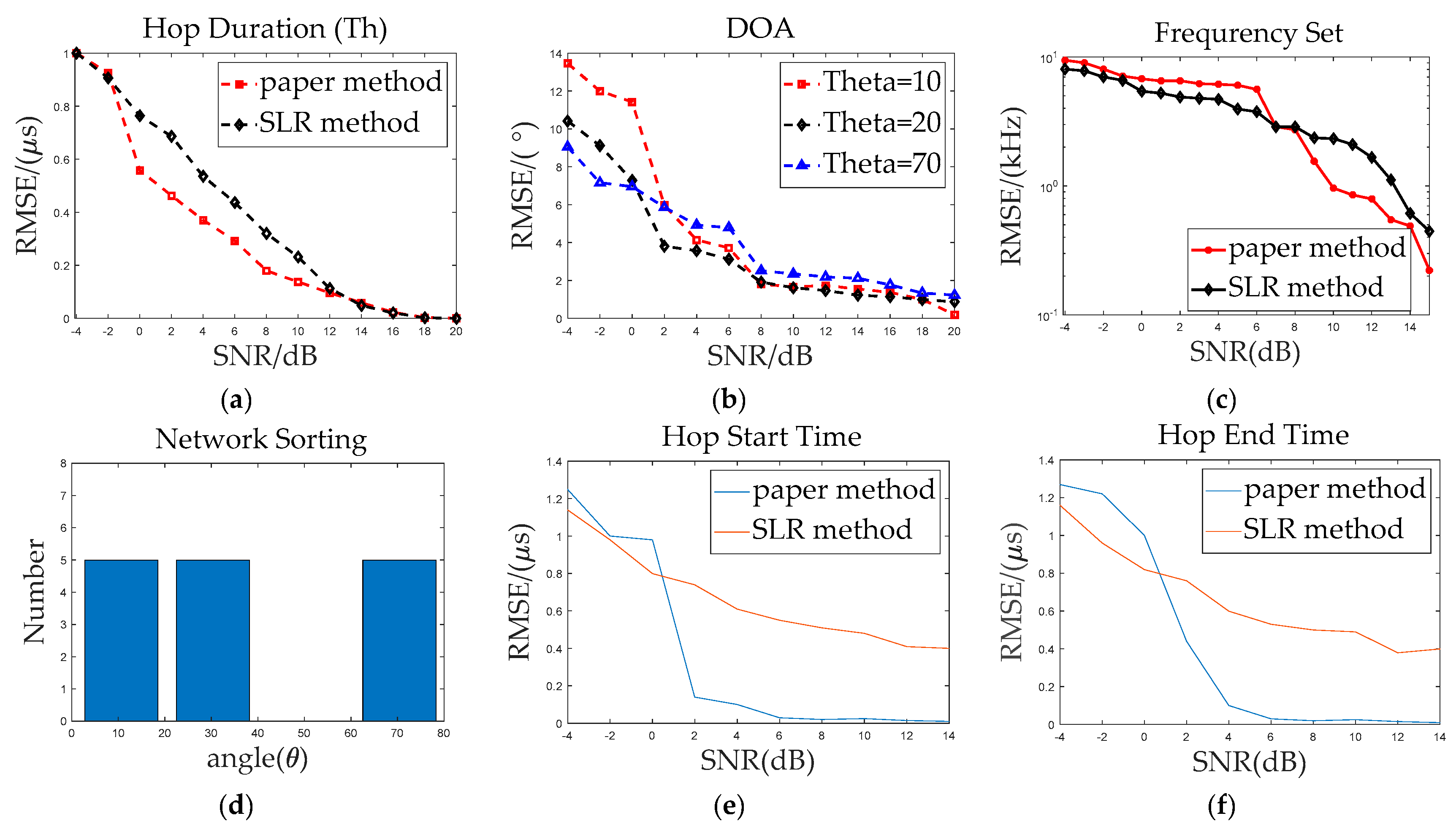
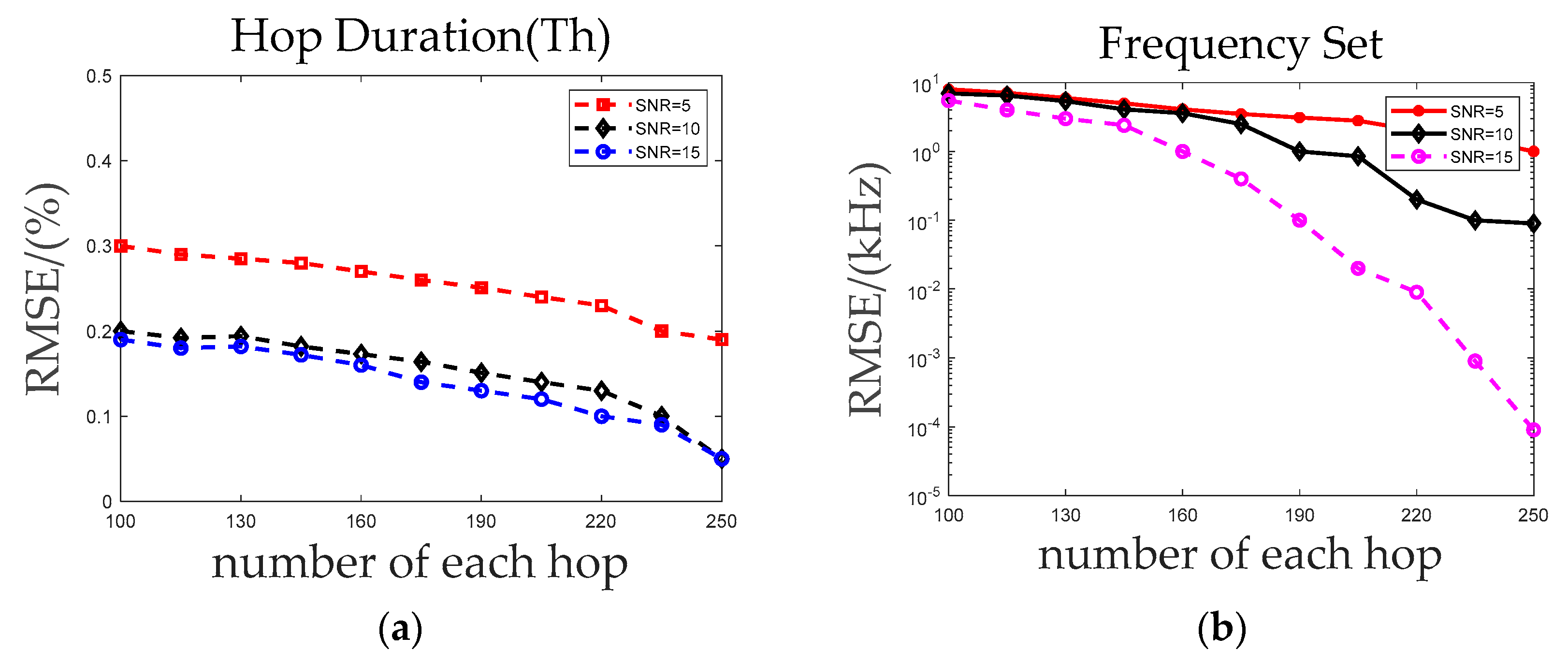
In order to adapt to the parameter estimation of multi-frequency hopping signals in more and more complex electromagnetic environment, based on the research of predecessors, this paper makes full use of the spatial domain information of array received signals. On the basis of the obtained matrix distribution of the space-time-frequency distribution, the matrix joint diagonalization algorithm is innovatively applied to the parameter estimation of multi-frequency hopping signals, and the root-MUSIC algorithm is used to complete the multi-frequency hopping signals. According to the estimated DOA of each hop, the k-means++ algorithm is used to complete the sorting of frequency hopping network stations. By setting up three sets of simulation experiments, the effectiveness of the proposed algorithm, the accuracy of the estimation and the robustness of the algorithm are verified. Through experimental simulation, it is found that when the SNR is −4 dB, the proposed finding “island” algorithm can correctly complete the estimation of the number of hops and the extract the self-terms time-frequency points, and the estimated accuracy is 70.43%, which is set for the text simulation conditions. the estimation error Th reaches 1.2 μs, and the estimated accuracy rate reaches 62%, which the DOA estimation error averages 9 ° , the estimated accuracy rate reaches 71%. The jump start time and the jump end time accuracy rate are 75.42% and 74.48%, and the frequency hopping frequency set estimation error is 1 MHz, which the accuracy rate reaches 73.26%. the average accuracy of the frequency hopping parameter estimation reaches 70.42%; when the SNR = 0 dB, the estimation accuracy reaches 82.46%. When the SNR = 5 dB, Th estimation error decreases to 0.025 μs, for which the accuracy rate is 94.5%; the DOA estimation error is 4 ° , which the accuracy rate is 94.28; the frequency hopping frequency set estimation error is reduced to 0.76 MHz, which the accuracy rate is 93.26%; the jump start time and the end time estimation accuracy rate are 96.12% and 95.96%, then the accuracy of the frequency hopping parameter estimation is 94.74%. As the signal-to-noise ratio increases, the estimation accuracy becomes higher and higher, and the proposed algorithm can be found to be effective for multi-hopping parameter estimation.

Author Contributions

Conceptualization, W.X. and D.Z.; Funding acquisition, J.W. and Q.G.; Methodology, J.W. and Q.G. and D.Z.; Software, D.Z.; Validation, Q.G. and D.Z.; Supervision W.X., Writing—original draft, D.Z.; and Writing—review and editing, D.Z. and W.X.

Funding

This research was funded by the Central University Basic Research Business Expenses Special Fund Project (No.HEUCFG201832), the National Key Research and Development Program of China (No.2016YFC0101700), the Heilongjiang Province Applied Technology Research and Development Program National Project Provincial Fund (No.GX16A007), State Key Laboratory Open Fund (No.702SKL201720).

Conflicts of Interest

The authors declare no conflict of interest.

References

  1. Yun-Bin, Y.; Qing-Min, T. DOA estimation methods of FH signals and follower jamming signals. J. Nav. Univ. Eng. 2016, 28, 228–234. [Google Scholar]
  2. Song, H.-Y.; Yang, C.-Y. Vector-sensor array DOA estimation using spatial time frequency distributions. In Proceedings of the 2018 IEEE International Conference on Consumer Electronics-Taiwan, Taichung, Taiwan, 19–21 May 2018; Volume 12, pp. 120–125. [Google Scholar]
  3. Zhu, M.; Qi, Y.; Zhang, X. A New Interpretation of S-Transform Spectrum: Phase Hopping Analysis and Estimation. Chin. J. Electron. 2019, 28, 338–343. [Google Scholar] [CrossRef]
  4. Kunfeng, Z.; Ying, G.; Zisen, Q. parameter estimation for multiple frequency-hopping signals based on sparse Bayesian reconstruction. J. Huazhong Univ.Sci. Technol. 2014, 45, 45–47. [Google Scholar]
  5. Sabra, K.G.; Anderson, S.D. Subspace array processing using spatial time-frequency distributions: Applications for denoising structural echoes of elastic targets. J. Acoust. Soc. Am. 2014, 135, 2821–2835. [Google Scholar] [CrossRef] [PubMed]
  6. Li, C. Directions of arrival estimation for multicomponent frequency-hoppingsignals based on spatial time-frequency analysi. Syst. Eng. Electron. 2011, 33, 42–45. [Google Scholar]
  7. Zuo, L.; Pan, J.; Ma, B.Y. Parameter Estimation of Multiple Frequency-Hopping Signals with Two Sensors. Sensors 2018, 18, 1088. [Google Scholar] [CrossRef] [PubMed]
  8. Feng, T.; Yuan, C.-W. Blind parameter estimation of frequency-hopping signals based on the time–frequency distribution maxima. Acta Electron. Sin. 2012, 39, 2921–2925. [Google Scholar]
  9. Guido, R.C. Practical and Useful Tips on Discrete Wavelet Transforms. IEEE Signal Process. Mag. 2015, 32, 162–166. [Google Scholar] [CrossRef]
  10. Liang, Z.-J.; Lv, M. A joint rapid parameter estimate method of frequency-hopping signals. In Proceedings of the 2012 International Conference on Control Engineering and Communication Technology, Shenyang, China, 7–9 December 2012; pp. 952–954. [Google Scholar]
  11. Zhang, H.-X.; Chen, C.-F.; Wang, H.-Q. A parameter estimation method for FH signal based on SPWVD. J. China Univ. Posts Telecommun. 2011, 18, 133–136. [Google Scholar] [CrossRef]
  12. Yang, Y.C.; Sun, X.L.; Zhong, Z.G. A Parameter Estimation Algorithm for Frequency-Hopping Signals with alpha Stable Noise. In Proceedings of the 2018 IEEE 3rd Advanced Information Technology, Electronic and Automation Control Conference (IAEAC), Chongqing, China, 12–14 October 2018; pp. 1898–1904. [Google Scholar]
  13. Guariglia, E. Harmonic Sierpinski Gasket and Applications. Entropy 2018, 20, 714. [Google Scholar] [CrossRef]
  14. Boashash, B. Time-Frequency Signal Analysis and Processing: A Comprehen-Sive Review, 2nd ed.; Elsevier: Amsterdam, The Netherlands, 2015; pp. 19–21. [Google Scholar]
  15. Hlawatsch, F.; Auger, F. Time-Frequency Analysis; John Wiley Sons: Hoboken, NJ, USA, 2010; Volume 36, pp. 142–145. [Google Scholar]
  16. Kanaa, A.; Sha’ameri, A.Z. A robust parameter estimation of FHSS signals using time-frequency analysis in a non-cooperative environment. Phys. Commun. 2018, 26, 9–20. [Google Scholar] [CrossRef]
  17. Belouchrani, A.; Amin, M. Blind source separation based on time-frequency signal representation. IEEE Trans. Signal Process. 1998, 46, 2888–2898. [Google Scholar] [CrossRef]
  18. Belouchrani, A.; Amin, M.G. Time-frequency MUSIC. IEEE Trans. Signal Process. Lett. 1996, 6, 109–110. [Google Scholar] [CrossRef]
  19. Qiang, L.; Yun, L.; Hang, C. Direction of arrival estimation using array model in time-frequency domain. In Proceedings of the 2010 International Conference on Audio, Language and Image Processing, Shanghai, China, 23–25 November 2010; pp. 1112–1116. [Google Scholar]
  20. Pinto, F.; Vetterli, M. Space-time-frequency processing ofacoustic wave fields: Theory, algorithms, and applications. IEEE Trans. Signal Process. 2010, 58, 4608–4620. [Google Scholar] [CrossRef]
  21. Xiong, B.; Zhao, X.; Liu, H.W. DOA estimation of LFM signals. In Proceedings of the International Conference on Wireless CommunicationsNetworking and Mobile Computing, Shenzhen, China, 23–25 September 2010; pp. 1–3. [Google Scholar]
  22. Guido, R.C.; Addison, P.S.; Walker, J. Introducing Wavelets and Time-Frequency Analysis Wavelet-Related Technologies in Biomedical Signal Processing. IEEE Eng. Med. Biol. Mag. 2009, 28, 13. [Google Scholar] [CrossRef] [PubMed]
  23. Liu, Z.M.; Huang, Z.T.; Zhou, Y.Y. Hopping instants detection and frequency tracking of frequency hopping signals with single or multiple channels. IET Commun. 2012, 6, 84–89. [Google Scholar] [CrossRef]
  24. Junbo, L.; Daifeng, Z. Spatial Time-Frequency MUSIC Algorithm in Stable Distribution Noise Environment. In Proceedings of the 2013 International Conference on Mechatronic Sciences, Electric Engineering and Computer (MEC), Shenyang, China, 20–22 December 2013; Volume 23, pp. 42–45. [Google Scholar]
  25. Roinila, T.; Messo, T.; Luhtala, R.; Scharrenberg, R.; de Jong, E.C.W.; Fabian, A.; Sun, Y. Hardware-in-the-Loop Methods for Real-Time Frequency-Response Measurements of on-Board Power Distribution Systems. IEEE Trans. Ind. Electron. 2019, 66, 5769–5777. [Google Scholar] [CrossRef]
  26. Padhi, T.; Chandra, M. Cascading time-frequency domain filtered-x LMS algorithm for active control of uncorrelated disturbances. Appl. Acoust. 2019, 149, 192–197. [Google Scholar] [CrossRef]
  27. Aykin, I.; Krunz, M.; Xiao, Y. Adaptive frequency-hopping schemes for CR-based multi-link satellite networks. Int. J. Satell. Commun. Netw. 2018, 36, 315–331. [Google Scholar] [CrossRef]
  28. Li, J.; Zhang, H.; Wang, P.F. Blind separation of temporally correlated noncircular sources using complex matrix joint diagonalization. Pattern Recognit. 2019, 87, 285–295. [Google Scholar] [CrossRef]
  29. Wei, Z.; Yu, W. Parameter Estimation Method of Multiple Frequency-hoppingSignals Based on OMP-SLR. Signal Inf. Process. 2018, 48, 871–875. [Google Scholar]
  30. Zhao, L.; Wang, L.; Bi, G.; Zhang, L.; Zhang, H. Robust Frequency-Hopping Spectrum Estimation Based on Sparse BayesianMethod. IEEE Trans. Wirel. Commun. 2015, 14, 781–793. [Google Scholar] [CrossRef]
Figure 1. The figure shows the system components.
Symmetry 11 00648 g001
Figure 2. Time-Frequency Model Diagram of Frequency Hopping Signal. This picture shows the law of signal frequency changing with time. (a) There are three frequency hopping signals in the graph. (a) total of 1250 time points are taken in the time domain. Each hop consists of 250 time points. (b) There are 25 time points in the graph, and each hop consists of 5 time points.
Symmetry 11 00648 g002
Figure 3. Space-time frequency distribution diagram of multi-hop frequency signal. (a) When SNR = 0 dB, the space-time-frequency distribution of the signal, (b) the time-frequency distribution of the signal after threshold transformation.
Symmetry 11 00648 g003
Figure 4. Space-time frequency distribution diagram of multi-hop frequency signal. (a) The figure is a space-time-frequency map of time-hopping signal after threshold processing when SNR = 0 dB, which is composed of self-term time-frequency points;(b) the figure is a space-time-frequency distribution map which is composed of only 0,1 elements after threshold processing and removing part of noise.
Symmetry 11 00648 g004
Figure 5. Space-time-frequency distribution with only 0,1 elements. (a) there is three hops surrounded by red frame in the graph, (b) there are four hops in the graph.
Symmetry 11 00648 g005
Figure 6. The rectangular process diagram of hop space-time frequency value. (ac) shows how to construct a space-time-frequency matrix from the extracted space-time-frequency values of each hop.
Symmetry 11 00648 g006
Figure 7. The corresponding diagram of each hop in the space-time frequency matrix of the frequency hopping signal.
Symmetry 11 00648 g007
Figure 8. Space-time-frequency diagram composed of self-term time-frequency points. (a) SNR = −3 dB, Space-time-frequency-diagram; (b) SNR = −2 dB, Space-time-frequency-diagram; (c) SNR = 5 dB, Space time frequency diagram.
Symmetry 11 00648 g008
Figure 9. Simulation results diagram.the graph shows the relationship between parameter estimation accuracy and signal-to-noise ratio. (a) The diagram shows the curve of hop duration (Th) estimation with SNR; (b) the diagram shows the curve of direction of arrival (DOA) with SNR; (c) the diagram shows the curve of frequency estimation with SNR; (d) the diagram shows the results of the frequency hopping station; (e) the diagram shows the curve of hopping start time with SNR. (f) the diagram shows the curve of hopping end time with SNR
Symmetry 11 00648 g009
Figure 10. Parameter estimation accuracy rate with frequency hopping duration change graph. The figure shows the accuracy of the frequency hopping parameter estimation with the frequency hopping time. (a) Frequency hopping period estimation accuracy varies with frequency hopping duration (b) Estimation accuracy of frequency hopping frequency set varies with frequency hopping duration.
Symmetry 11 00648 g010
Table 1. Multi-hop frequency signal parameter table. The table describes the jump frequency and frequency hopping period information of the selected simulation signal.
Group F s   ( MHz ) t (μs)SignalHopping Duration ( T h )Normalized Frequency f h , k   ( MHz )
Group110012.5 F h 11 250[0.50,0.86,0.52,0.30,0.74]
F h 12 250[0.76,0.20,0.72,0.42,0.90]
F h 13 250[0.96,0.36,0.10,0.62,0.52]
Group210012.5 F h 21 250[0.50,0.86,0.52]
F h 22 250[0.76,0.20,0.72,0.42]
F h 23 250[0.96,0.36,0.10,0.62,0.52]
Group31005 F h 31 100[0.50,0.86,0.52,0.30,0.74]
F h 32 100[0.76,0.20,0.72,0.42,0.90]
F h 33 100[0.96,0.36,0.10,0.62,0.52]
Table 2. Hop number estimation result table. The table shows the estimation of the number of hops of frequency hopping signals under different SNRs.
SNR (dB)Simulation Hop Number ( N o )Estimation Hop Number ( N e )Accuracy (%)
−10153030.42%
−5152060.28%
−4151670.43%
−3151595.56%
0121299.41%
51212100%
61212100%

