When Considering More Elements: Attribute Correlation in Unsupervised Data Cleaning under Blocking

Abstract

In banks, governments, and internet companies, due to the increasing demand for data in various information systems and continuously shortening of the cycle for data collection and update, there may be a variety of data quality issues in a database. As the expansion of data scales, methods such as pre-specifying business rules or introducing expert experience into a repair process are no longer applicable to some information systems requiring rapid responses. In this case, we divided data cleaning into supervised and unsupervised forms according to whether there were interventions in the repair processes and put forward a new dimension suitable for unsupervised cleaning in this paper. For weak logic errors in unsupervised data cleaning, we proposed an attribute correlation-based (ACB)-Framework under blocking, and designed three different data blocking methods to reduce the time complexity and test the impact of clustering accuracy on data cleaning. The experiments showed that the blocking methods could effectively reduce the repair time by maintaining the repair validity. Moreover, we concluded that the blocking methods with a too high clustering accuracy tended to put tuples with the same elements into a data block, which reduced the cleaning ability. In summary, the ACB-Framework with blocking can reduce the corresponding time cost and does not need the guidance of domain knowledge or interventions in repair, which can be applied in information systems requiring rapid responses, such as internet web pages, network servers, and sensor information acquisition.

1. Introduction

Data cleaning means the examination and repair of identifiable errors by manual or technical means to improve data quality [1]. In banks, governments and internet companies, the increasing demand for data in various information systems and constantly shrinking of the cycle for data collection and update make the data scale expand, and can even lead to a variety of “dirty data”, which are often fatal in a data-intensive enterprises and may cause huge economic losses. It’s the key and the purpose of doing data cleaning to solve the data quality problems accompanying big data and clean “dirty data” in datasets How to solve data quality problems accompanying big data and clean “dirty data” in datasets is the key and the purpose of data cleaning research [2]. The data mining method is usually used to obtain valuable information from datasets; however, because “dirty data” cannot correctly express the true state of elements and destroys the relationship between objective elements, it makes the results of data mining untrustworthy, which brings great difficulties to the decision-making process [3].

Referring to supervised learning [4,5] and unsupervised learning [6,7,8] in machine learning, we divide the data cleaning into two different forms: supervised and unsupervised data cleaning. Here, the difference is that the supervised and unsupervised data cleaning is not determined by whether training sets with accurate labels are required, but according to whether external interventions in the cleaning processes exist. Supervised data cleaning means cleaning the “dirty data” by first pre-specifying business rules or introducing manual interventions, then dividing these “dirty data” into specific data quality dimensions and selecting appropriate methods to repair them, e.g., repairing the inconsistent data violating conditional functional dependencies [9] and data currency improvement by specifying the timing series [10], which usually achieves better repair results because of sufficient prior knowledge before repair. Furthermore, the review and modification of the results by the domain experts after the repair can further improve the accuracy. However, not all the data cleaning processes are always supervised, and some domain-independent erroneous data which are violating basic database constraints or system semantics can also be detected in a data checking process. These domain-independent erroneous data are difficult to be classified into traditional ones because of the lack of business rules, which makes it difficult to repair relying on existing business rules. The data cleaning for these domain-independent erroneous data can be regarded as an unsupervised data cleaning process. Unlike traditional data quality problems, the detection of domain-independent erroneous data does not depend on business rules specified by business personnel, but on basic database constraints and system semantics. Meanwhile, their repair does not rely on the existing business rules too. Therefore, they are a kind of common erroneous data, and their repair may be more difficult without the participation of business rules.

In this case, our research focuses on data quality problems and proposes an unsupervised data cleaning framework. It takes the corresponding conflict-free data set without “dirty data” as the training set and learns the correlation among attributes by machine learning to guide the subsequent repair. By keeping the repairability, we design blocking methods to reduce the time complexity, so that it can be applied to large-scale datasets. The whole framework does not require to pre-specify business rules or manual interventions, and it is an automatic and common framework, which ensures real-time performance.

1.1. Problem Description

In supervised data cleaning, different types of data quality problems are usually divided into different dimensions. The classical dimension includes indicators such as accuracy, completeness, consistency, normalization, and timeliness [11]. Under these circumstances, researchers detect and repair data quality problems by specifying multiple business rules or logical relationships among data, and usually adopt different methods for different dimension problems, e.g., missing data filling in the multi-view and panoramic dispatching [12,13], and inconsistent data repair under the distributed big data [14]. Unlike the supervised data cleaning, the unsupervised data cleaning can essentially be seen as a repair way which relies solely on the dataset itself. Due to the lack of sufficient domain knowledge to specify the corresponding business rules for the erroneous data, we believe that different dimension problems can be repaired by a similar method in the unsupervised environment. Therefore, we reclassified data quality problems into the following dimensions:

(1) Redundancy error

Similar to traditional data quality dimensions [13], the redundancy error data in unsupervised cleaning also means that multiple identical or similar records are generated for the same entities [15]. Because it contains useless or duplicate information, the redundant data wastes storage space and reduces data availability. Entity resolution (ER) technology is usually used to repair this kind of data error [15,16,17].

(2) Canonicalization error

Canonicalization errors indicate an inconsistency caused by different recording methods for the same attributes in the process of data merging or multi-source data fusion [11]. The values of these error elements are usually correct, but due to the lack of standardization, they are determined as a data error during the detection process. In this case, data standardization can solve these errors well.

(3) Strong logic error

Strong logic errors have two meanings. Firstly, different from canonicalization errors and redundancy errors, they are a kind of error type with a truth value error. Secondly, there is a strong logical correlation between the attribute of the data error and other attributes in the dataset (e.g., the left-hand side (LHS) and right-hand side (RHS) attributes of a conditional functional dependency: the birthday, and age attributes of a company’s staff). Such strong logical correlation is easy to obtain or specify from the given dataset and can guide the cleaning process directly. For strong logic errors in domain-independent erroneous data, these strong logic relationships between attributes can be transformed into business rules, and we can adopt an existing supervised method to reduce the repair difficulty according to the transformed rules.

(4) Weak logic error

Weak logic errors in datasets are the focus of our attention, and they are also a kind of error type with truth value error, but there is a weak logic correlation among attributes, which are also the inherent relationship (e.g., the company address and home address of a staff, and the correlation between an employee’s education and monthly salary). Although the data elements with weak logic errors seem to be unrelated to other attributes in the dataset, there is a certain internal correlation between the data elements, and such logical relations are also inherent in the dataset, but they are difficult to discover for directly guiding the repair of the erroneous data.

In summary, we can adopt methods in supervised data cleaning for the redundancy error, canonicalization error, and strong logic error of domain-independent erroneous data. However, we have to design a new method for weak logic errors, because it is difficult to transform weak logic relations into business rules directly. Therefore, the purpose of this paper is to propose an unsupervised data cleaning framework for weak logical error data in datasets, so that the repair results can make full use of the correlation among data elements.

The following relation schema is given to illustrate the expression of the erroneous elements and the corresponding cleaning processes.

HousePrices (Id, MSSubClass, MSZoning, Street, LotShape, CentralAir, BldgType, SalePrice)

The meanings, value types, and abbreviations of every attribute in the relation schema are shown in

Table 1. HousePrices attributes description.

Attributes	Meanings	Value Types	Abbreviations
Id	the building number	numeric	ID
MSSubClass	the building class	numeric	MC
MSZoning	the general zoning classification	text	MZ
Street	type of road access	text	ST
LotShape	general shape of property	text	LS
CentralAir	central air conditioning	Boolean	CA
BldgType	type of dwelling	text	BT
SalePrice	the property’s sale price in dollars	numeric	SP

.

For description convenience, the subsequent attributes’ descriptions are all represented by the abbreviations in this paper; for example, the LS and BT indicate the LotShape attribute and the BldgType attribute in HousePrices, respectively.

For example, part of the tuple in the HousePrices dataset was selected here to give a partial data instance in the relational schema, which is shown in

Table 2. HousePrices data instance.

ID	MC	MZ	ST	LS	CA	BT	SP
1	60	RL	Pave	Reg	Y	1Fam	200,000
2	20	RL	Pave	Reg	*	1Fam	181,500
3	60	RM	Pave	IR1	Y	1Fam	140,000
4	*	RL	Grvl	IR1	Y	*	250,000
5	60	FV	Pave	IR1	N	1Fam	140,000
6	50	RM	Pave	Reg	N	1Fam	307,000
7	20	*	Pave	IR2	Y	Duplex	200,000
8	60	RM	Grvl	IR2	Y	1Fam	129,500
9	50	FV	Pave	Reg	Y	Duplex	129,500
10	20	RL	Pave	IR1	N	1Fam	345,000

* were used to simulate the erroneous data in HousePrices instance.

. MSZoning means identifies the general zoning classification of the sale, and RL, RM, FV are residential low density, residential medium density and floating village residential respectively. Street means type of road access to property, and Grvl is gravel, while Pave is paved. LotShape means general shape of property, and Reg, IR1, IR2 are regular, slightly irregular and moderately respectively. Since elements in datasets do not appear randomly, there can be some inherent correlation between the erroneous element and other elements in data instances, and these elements can be treated as weak logic errors in the unsupervised environment. When lacking sufficient domain knowledge and interventions, we hope to take the correlation in datasets into account and obtain the most relevant repair results.

In this paper, we express the erroneous dataset (EDS) in datasets as follows.

$$EDS=\left\{\left(t_i,A_j\right),\left(t_k,A_l\right),\dots ,\left(t_m,A_n\right)\right\}$$

(1)

In Equation (1), $t_i$, $t_k$, and $t_m$ represent the unique tuple identifiers of erroneous data, and $A_j$, $A_l$, and $A_n$ represent the corresponding attributes. We can locate the erroneous data in datasets through the two-tuples expression, for example, the EDS in HousePrices instance can be expressed as

$$EDS=\left\{\left(t_2,CA\right),\left(t_4,MC\right),\left(t_4,BT\right),\left(t_7,MZ\right)\right\}.$$

1.2. Research Status

The current data cleaning research aims to divide different data quality problems into datasets, and adopts different repair methods in the traditional dimension, e.g., for the redundant data in datasets, Abu Ahmad et al. [16] proposed a multi-attributes weighted rule system (MAWR) to solve different entities with the same name in entity resolution processes, and these entities have no identifier keys, and Wang et al. [17] proposed an entity resolution method based on sub-graph cohesion to solve the transitivity problems in resolution. For the inconsistent data in datasets, Brisaboa et al. [18] proposed a rank-based data cleaning strategy to solve the inconsistent data in spatial databases and improve the efficiency by dynamic adjustment, and Xu et al. [19] proposed an inconsistent data repair method based on the minimum cost, and selected an element to repair by computing the change amount of conflict elements before and after all candidate repair values updating.

Different from the supervised data cleaning process, the unsupervised data cleaning lacks sufficient domain knowledge and interventions, so different data quality problems in the traditional dimension can be repaired by similar methods. For the unsupervised data cleaning, the common methods can be divided into two categories. One is to use data mining (such as association rules mining [20,21], frequent pattern mining [22], etc.) to mine out possible business rules from datasets and transforms the unsupervised data cleaning into supervised. However, there are two main disadvantages in these methods: (1) The support threshold setting in data mining has a great impact on results; too large or too small thresholds will affect its credibility and effectiveness. In this case, a different combination of thresholds can obtain a different mining result, which makes the results subjective. (2) The data mining results are not all “equality constraints” like conditional functional dependencies, which cannot guide the repair process directly, but also need to integrate a decision tree [23], interpolation [24] or other methods. The other is to use the dataset itself to repair data errors, e.g., Reference [25] proposes a data cleaning framework, Boostclean, based on machine learning, which improves the accuracy of detection and repair, and Reference [26] proposed a regression-based method to repair the erroneous data in datasets, while using an interactive method to correct the unsatisfactory data, which combines the supervised and unsupervised ideas. These kinds of methods do not require an additional training set in the repair processes, but the time complexity is relatively high. Therefore, we hold the opinion that, in unsupervised cleaning, the corresponding conflict-free dataset without “dirty data” can be regarded as the training set to learn the correlation, and then we repair the erroneous data by the learning correlation, which may obtain better results.

In summary, the current data cleaning research mainly has the following three problems: (1) Different algorithms can better repair the erroneous data in the dataset, but the complexity is also high, which cannot be applied to some large datasets. (2) When selecting a candidate repair element, less consideration is taken of the correlation among the data, so that these methods can obtain repair results, but their authenticity remains to be further questioned. (3) Different repair methods are proposed for different traditional dimension problems, but less attention is paid to data cleaning in the unsupervised environment. Because there are insufficient domain knowledge and manual interventions, it can be much more difficult to repair the erroneous data in the unsupervised environment.

In our research, we hold that it is more credible to repair the erroneous data in datasets by learning the inherent correlation under the unsupervised environment. The main idea is: For the given dataset and EDS, the conflict-free dataset ($I_{cf}$) that has deleted the erroneous data tuples is firstly partitioned by using the data partitioning method to reduce the complexity of the repair algorithm. Then, we adopt the symmetric uncertainty method in information theory to learn the correlation among attributes and repair the erroneous data based on the learning correlation in each block. Finally, we select the most frequent repair value in all blocks as the target value of the erroneous data. This method integrates the data blocking and attribute correlation ideas and takes the conflict-free data subset ($I_{cf}$) as the training set to solve the problem of insufficient training sets in unsupervised cleaning. Moreover, it does not require any additional domain knowledge and manual interventions, which provides high real-time algorithm and it can be applied to large-scale information systems requiring a rapid response. We will illustrate the blocking methods and specific repair processes in Section 2.

1.3. Purpose and Structure of This Paper

The purpose of this paper is to propose a data cleaning framework for weak logic errors under unsupervised environments. The main contributions and innovations are:

(1) We divide the data cleaning into supervised and unsupervised forms according to whether there are intervention processes and reclassify the data quality problems in datasets to clarify the application scenarios of our proposed methods.

(2) For the unsupervised data cleaning, we take the conflict-free data subset as the training set to learn the attribute correlations among elements and repair the erroneous data through the learning correlation, which makes repair results satisfy the inherent rules of the datasets under the premise of meeting requirements.

(3) We adopt data blocking technology to reduce the cleaning complexity and put forward three different blocking methods to discuss the impact of blocking on repair ability so that the algorithm can be applied to large-scale datasets.

The rest of this paper is structured as follows:

In Section 2, we first propose the data cleaning framework—attribute correlation-based (ACB)-Framework—for weak logic errors in unsupervised data cleaning, and design two sub-modules in the framework. To facilitate the reader’s understanding and for reproduction, we provide an example to illustrate the blocking and cleaning process. Then, we implement the blocking and cleaning algorithms in the ACB-Framework and analyze their convergence and time complexity. In Section 3, to compare the influence of the blocking methods with different clustering accuracies on the data cleaning results, the ACB-Framework is carried out in different conditions. In Section 4, we first summarize the experimental results and give possible explanations. Then, we analyze the advantages and disadvantages of the ACB-Framework and put forward the subsequent directions for improvement. At last, we comb the structure and summarize the contributions of this paper in Section 5.

2. Materials and Methods

For weak logic errors in unsupervised data cleaning, we put forward an attribute correlation-based framework (ACB-Framework) under blocking, then analyze and design the blocking and cleaning modules in the framework to improve the data quality and data availability.

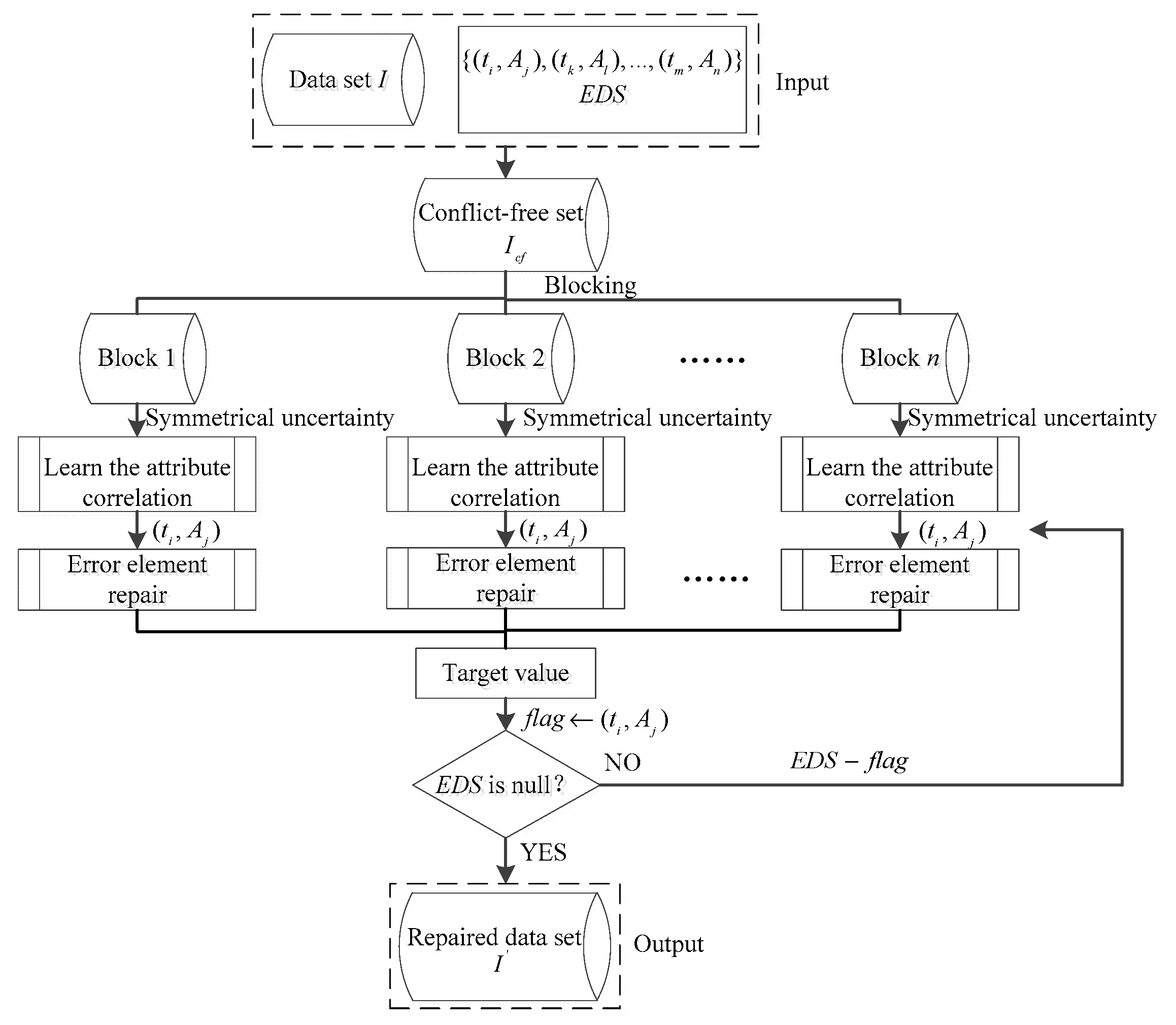
2.1. Design of the ACB-Framework

In the unsupervised environment, we learned the attribute correlation from conflict-free data sets, and guide the subsequent repair process according to the attribute relevance of learning, which can improve the data quality in datasets. However, when the data scale is large, repair methods, which directly learn the correlation and repair in $I_{cf}$, can be very complex and inefficient. In this case, we adopted data blocking methods [15,27,28] to reduce the complexity on the basis of maintaining the repair ability, so that the ACB-Framework can be applied to large-scale datasets.

In a data cleaning process, since some “dirty data” exists in datasets, we should consider the following three aspects when designing blocking methods and subsequent data cleaning:

(1) How should datasets with erroneous data be blocked?

Because datasets with erroneous elements usually contain some wrong attribute values, which will affect the data blocking accuracy, we take the corresponding conflict-free data subset without error tuples ($I_{cf}$) as the training set, and conduct blocking in $I_{cf}$.

(2) Which block should the erroneous data be repaired in?

Selecting different data blocks to repair the erroneous data can directly affect the repair results, and the difference of repair validity before and after blocking is also an important index to evaluate different blocking methods. The intuitive method is to select the most relevant and nearest block to the erroneous data tuple so that the repair results can satisfy the correlation requirements. However, because of some wrong elements in the erroneous tuple, other attributes in the erroneous tuple are most relevant to a data block, which does not mean that the erroneous elements are also most relevant to the data block. In this case, we put erroneous elements in every data block to repair and selected the most frequent repair value in different data blocks as the final target value, which can largely eliminate the impact of blocking methods on data repair results.

(3) How to assign the attribute weights in the blocking processes?

Data blocking is substantially similar to a clustering process. When computing the similarities among multiple tuples, it is usually necessary to know the attribute weights in a dataset. The most common method to assign the attribute weights is through expert experience, which makes it very subjective, and the assignment of attribute weights itself is a kind of manual intervention. Therefore, we choose the Jaccard method to avoid the setting of attribute weights.

In summary, our ideas can be concluded as follows. We first block the $I_{cf}$ through the methods proposed in Section 2.2. Then, we use the symmetric uncertainty in information theory to learn the correlation among attributes in every data block and put the erroneous element into every data block for repair. Finally, we select the most frequent repair value in different data blocks as the final target value, and remove the repaired element from the EDS. While the EDS is empty, we can obtain the repaired dataset. The flow of the ACB-Framework is shown in Figure 1.

In Figure 1, the ACB-Framework takes the given dataset I and the EDS as input, and outputs the repaired dataset I′, which can be divided into two modules: blocking and data cleaning. In the unsupervised environment, the framework repairs the erroneous data in the EDS through the attribute correlation, which selects the most relevant element in the blocks to replace the original element in nature. Therefore, there may still be a small number of erroneous data remaining after repair. In order to keep the convergence of the ACB-Framework, we adopt a label flag marking the repaired elements to ensure every data element are repaired at most once.

2.2. The Blocking Module

According to the ACB-Framework in Figure 1, we adopt blocking methods to reduce the complexity of the data cleaning processes. In order to test the impact of different clustering accuracies on data cleaning, we designed three different blocking methods.

2.2.1. Design of Blocking Algorithms

Data blocking is the key to reducing the time complexity of the cleaning processes. It always costs much time to learn the attribute correlation from the $I_{cf}$ directly, so that it cannot be applied to a large-scale dataset. In this case, by designing reasonable blocking algorithms, the ACB-Framework can reduce the time complexity on the basis of keeping the repair ability. We believe three basic principles should be followed when designing blocking methods:

(1)

Blocking is a pretreatment process in data cleaning to reduce the time complexity, so we should choose algorithms with low complexity.

(2)

The repair ability of data cleaning algorithms cannot be significantly reduced after blocking.

(3)

Blocking algorithms should improve the repair speed of erroneous data in datasets.

Data blocking is essentially similar to a clustering process, and we can get different results through blocking methods with different clustering accuracies. We hold the opinion that over-precise blocking results may destroy the correlation among elements in the original dataset and will reduce the repair ability, because they put all similar data tuples into a data block. To validate this idea, we designed three blocking methods with increasing clustering accuracy, and the time complexity of these three methods was gradually increased.

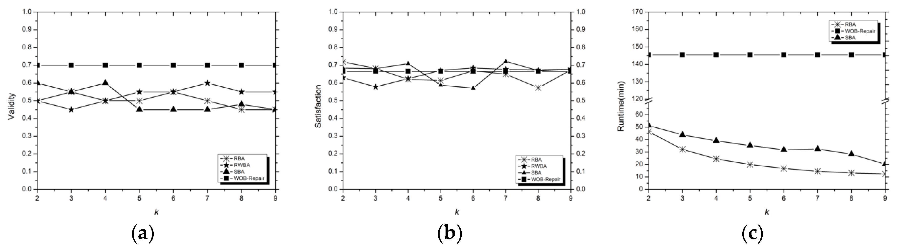
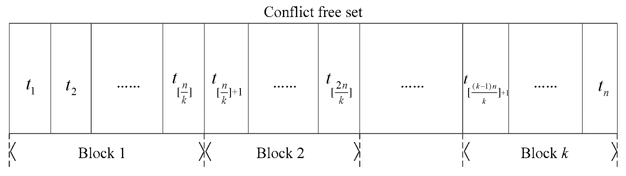
Random Blocking Algorithm (RBA)

The RBA is a very simple and fast blocking method, which can quickly divide a dataset into a specified number of blocks. Suppose there are n tuples in $I_{cf}$, the RBA equally divides the $I_{cf}$ into k blocks on the basis of ensuring the initial tuple order and puts all remaining tuples that cannot be divided exactly into the last data block. In this way, the tuple amounts in the first k − 1 blocks are all $\left[n/k\right]$, and the last block is no more than $\left[n/k\right]+k-1$, as shown in Figure 2.

Taking the HousePrices instance in Table 2 as an example, and the corresponding conflict-free subset $I_{cf}=\left\{t_1,t_3,t_5,t_6,t_8,t_9,t_{10}\right\}$, we specify the blocking amount k = 2, and the $I_{cf}$ can be divided into the following two blocks: Block 1 = $\left\{t_1,t_3,t_5\right\}$ and Block 2 = $\{t_6,t_8,t_9,t_{10}\}$.

The RBA takes the conflict-free dataset $I_{cf}$ and blocking amount k as input. The main idea is to divide the $I_{cf}$ into k blocks under keeping the original tuple order, which is shown in Algorithm 1.

Algorithm 1. The Random Blocking Algorithm (RBA) flow.

Input: conflict-free dataset $I_{cf}$, blocks amounts k Output: blocking results of RBA

01. // initialization 02. n=i=m=0; 03. // n is the tuples amounts in $I_{cf}$ 04. $n\leftarrow$tuples amount in $I_{cf}$; 05. // i is the tuples amounts of the first k − 1 blocks 06. $i\leftarrow$[n/k]; 07. // m=0,1,2,…,k − 1 08. Block m=($t_{i\left(m-1\right)+1},t_{im}$) in $I_{cf}$; 09. Block $k\leftarrow$remaining tuples in $I_{cf}$; 10. end;

In Algorithm 1, the L1 to L2 initialize the variables involved in the RBA; the L3 to L6 obtain the tuple amount n of $I_{cf}$ and compute the tuple amount i of the first k − 1 data blocks; the L8 to L10 do blocking for tuples in $I_{cf}$.

The RBA has the advantage of fast blocking speed and can partly retain the correlation among elements in the original dataset. However, its clustering accuracy is very poor, and the selection of the blocking amount k will directly affect tuples in a block, thus further affecting the accuracy of the attribute correlation learning from every data block. Therefore, we will analyze in detail the complexity of the RBA in Section 2.2.2, and discuss the impact of blocking amount k on data cleaning in Section 3.2.

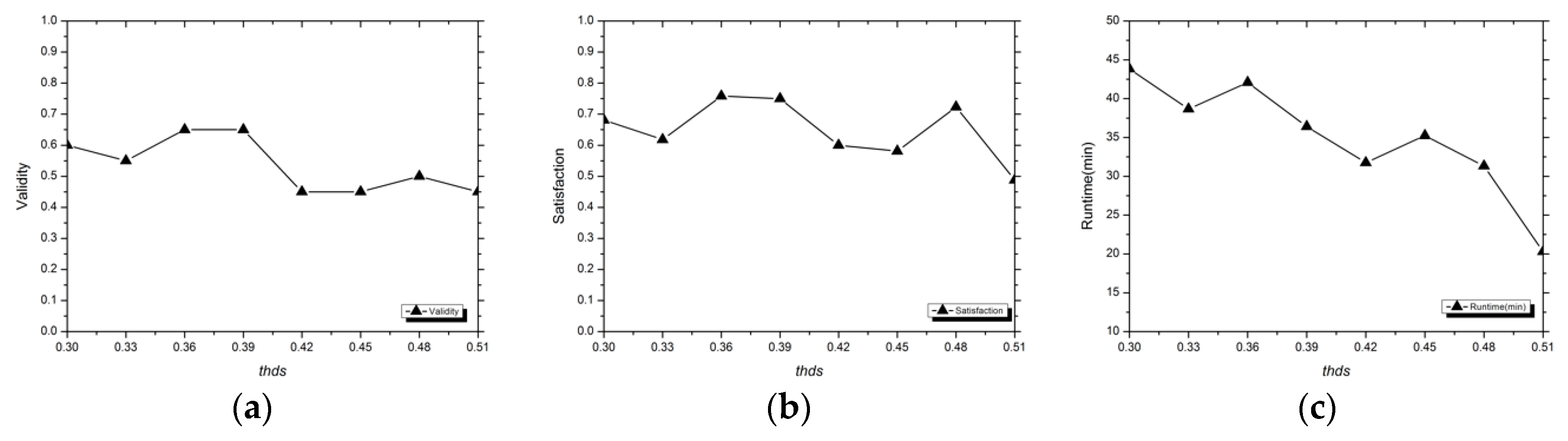
Similarity Blocking Algorithm, SBA

The SBA conducts blocking according to the similarities among tuples and puts tuples with high similarity into the same data block. Compared with the RBA, the SBA has better clustering accuracy, but also a higher time complexity. When designing a similarity function, a classic method is to set different functions for different attribute types and then design a comprehensive algorithm to combine the similarities of different attributes. However, this kind of method inevitably requires the attribute weights in datasets and has strong subjectivity. In this case, we adopt the Jaccard method to compute the similarities among tuples in $I_{cf}$. The mathematical definition is as follows:

$$sim\left(t_i,t_j\right)=\frac{\left|t_i=\left\{A_1,A_2,\dots ,A_N\right\}{\displaystyle \cap }{t}_j=\left\{A_1,A_2,\dots ,A_N\right\}\right|}{|t_i=\left\{A_1,A_2,\dots ,A_N\right\}{\displaystyle \cup }{t}_j=\left\{A_1,A_2,\dots ,A_N\right\}|}$$

(2)

When the tuples $t_i$ and $t_j$ are the same, the $sim\left(t_i,t_j\right)$=1 and the $sim\left(t_i,t_j\right)$=0 when they are totally different. Taking the tuples $t_1$ and $t_3$ of HousePrices instance in Table 2 as an example, the $sim\left(t_1,t_3\right)$ = 8/14 = 0.571.

The SBA takes the $I_{cf}$ and a matching determination threshold $th{d}_s$ as input. The main idea is to first select a data tuple from the candidate queue (CQ) as the blocking center $C_k$ and compute the similarities between the $C_k$ and other tuples in CQ. Then, we put all tuples satisfying the threshold $th{d}_s$ into a block and deleted them from the CQ. Similarly, other blocks can repeatedly be acquired until the CQ does not contain any tuples, which is shown in Algorithm 2.

Algorithm 2. The Similarity Blocking Algorithm (SBA) flow.

Input: conflict-free dataset $I_{cf}$, threshold $th{d}_s$ Output: blocking results of SBA

01. // initialization 02. $CQ$=null, k=1; 03. // add all tuples in $I_{cf}$ to candidate queue 04. $CQ\leftarrow$tuples in $I_{cf}$; 05. for $CQ!=$null        do 06.         $C_k\leftarrow$a random tuple in $CQ$; 07.         // add tuple $C_k$ to Block k 08.         Block $k\leftarrow$add $C_k$; 09.         $CQ$ = $CQ-C_k$; 10.         for $t_i\in CQ$        do 11.                 // the similarity between tuple $t_i$ and $C_k$ satisfies the given threshold 12.                 if($sim\left(t_i,C_k\right)\ge th{d}_s$)        do 13.                                 // add tuple $t_i$ to Block k 14.                                 Block $k\leftarrow$add $t_i$; 15.                                 $CQ$ = $CQ-t_i$; 16.                 end if; 17.         end for; 18.         k++; 19. end for; 20. end

In Algorithm 2, the L1 to L2 initialize the variables involved in the SBA; the L3 to L4 add all tuples of $I_{cf}$ into the candidate queue (CQ); the L5 to L9 randomly select a tuple from the CQ as the blocking center $C_k$ while the CQ is not empty, and delete it from the CQ after adding it to corresponding Block k; the L10 to L17 compute the similarities between the $C_k$ and other tuples in CQ, and remove all satisfying tuples from the CQ after putting them into the Block k; the L18 to L20 repeatedly acquire other blocks from the remaining CQ until the CQ is empty.

Compared with the RBA, the SBA method has better clustering accuracy, but also higher time complexity. While blocking, the SBA determines whether two tuples $t_i$ and $t_j$ in $I_{cf}$ matching by setting a threshold $th{d}_s$. The selection of $th{d}_s$ has a direct impact on blocking size and amount, and different thresholds may influence the repair ability of the data cleaning module too. Therefore, we will analyze in detail the complexity of the SBA in Section 2.2.2, and discuss the impact of $th{d}_s$ on the data cleaning in Section 3.2.

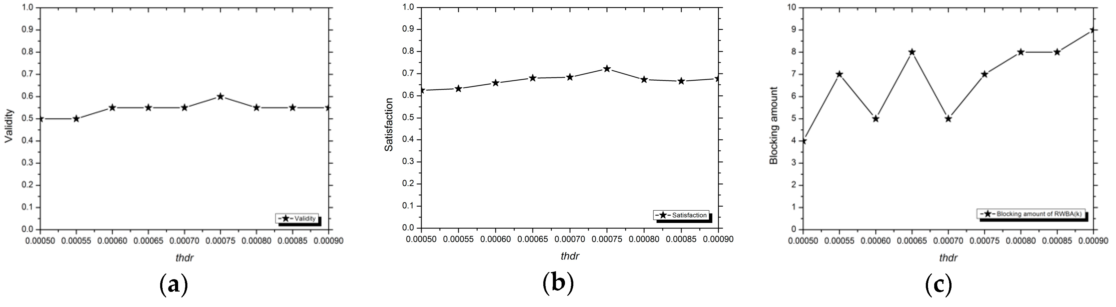
Random Walk Blocking Algorithm, RWBA

The RWBA first needs to establish a similarity graph for all tuples according to the similarity pairs, and then uses the structural information of the established graph to conduct blocking. In this paper, a similar pair of tuples $t_i$ and $t_j$ in $I_{cf}$ is expressed by the following triples.

$$similaritypair=[t_i,t_j,sim\left(t_i,t_j\right)]$$

(3)

where $t_i$ and $t_j$ represent any two tuples in $I_{cf}$, and the $sim\left(t_i,t_j\right)$ means the Jaccard similarity between them. Compared with the SBA, the random walk on a similarity graph considers not only the direct correlation between blocks and tuples, but also the indirect correlation through other tuples to blocks. Therefore, when computing the correlation degree between blocks and tuples, we use the random walk with the restart method to obtain the structural information in a similarity graph and take the stable probability of the random walk as the correlation degree. To distinguish the Jaccard similarities among tuples in the SBA, we express the correlation degree between a block n and tuple $t_i$ by random walk method as the $si{m}_{cd}\left(\mathrm{Block}n,t_i\right)$.

The random walk model [29] obtains the structural information in a similarity graph by simulating a random walk behavior. Given a similarity graph G and a random walker, the walker starts from one or a group of nodes with initial probabilities. During a transition process, the walker either arrives at its neighbor nodes in G with a certain probability $1-\mathsf{\alpha },$or returns to the initial nodes with a probability $\mathsf{\alpha }$ (i.e., the restart process). When the probability of the walker arriving at every node is stable, the random walk process ends and reaches a convergence state. We take the stable probability as the correlation degree between the initial node (nodes) and other nodes. In this way, we can make full use of the structural information in the similarity graph when computing the correlation degrees between blocks and tuples.

The similarity graph G(T,S), composed by similarity pairs, is a weighted and undirected graph, where the T represents the node set in G(T,S) (i.e., the tuple set, $t_i\in T$), and the S represents the similarity set among nodes (i.e., the weight of G(T,S) represents the similarity between the corresponding two tuples, $sim\left(t_i,t_j\right)\in S$). In order to facilitate descriptions, we will use the two words, node and tuple, without distinction.

The random walk with restart on the similarity graph G(T,S) is an irreducible, aperiodic, and finite Markov chain, so the convergence state must exist and be unique [30]. For an initial node set N ($N\in T$) in the G(T,S), let vector ${\pi }_0$ be the probability distribution of every node in the initial state, and the next state ${\pi }_1$ can be expressed as

$${\pi }_1=\left(1-\mathsf{\alpha }\right)\times P^T\times {\pi }_0+\alpha \times q$$

(4)

In Equation (4), the initial state ${\pi }_0$ and restart vector q are both column vectors in which the components corresponding to initial nodes set are $1/N$, and the other components are all 0. The restart probability $\mathsf{\alpha }$ = 0.15 [31] and $P$ is the state transition matrix on similarity graph G(T,S). The mathematical definition is as follows

$$P=\{P_{ij}|P_{ij}=w_{ij}/{\displaystyle \sum }{w}_{i\ast }\}$$

(5)

where the $w_{ij}$ is the corresponding weight of a similarity pair $t_i$ and $t_j$, i.e., the $sim\left(t_i,t_j\right)$.

The subsequent states ${\pi }_n$ on G(T,S) can be similarly computed by the Equation (4). When all nodes on the G(T,S) are in convergence, which is recorded as the vector ${\pi }_{\ast }$, the components of the ${\pi }_{\ast }$ are relatively stable and satisfy Equation (6).

$${\pi }_{\ast }=\left(1-\mathsf{\alpha }\right)\times P^T\times {\pi }_{\ast }+\alpha \times q$$

(6)

The RWBA takes the $I_{cf}$ and a matching determination threshold $th{d}_r$ as input. The main idea is to first compute all similarity pairs in $I_{cf}$ and establish a similarity graph G(T,S). Then we add all tuples in $I_{cf}$ into the candidate queue (CQ) and randomly select a tuple from the CQ as the blocking center $B_k$. Finally, we compute the correlation degrees between the $B_k$ and other tuples in CQ by the random walk with the restart method, and remove all satisfying tuples from the CQ after putting them into a block. Similarly, we can obtain other blocks from the remaining CQ until the CQ is empty. The RWBA flow is shown in Algorithm 3.

Algorithm 3. The Random Walk Blocking Algorithm (RWBA) flow.

Input: conflict-free dataset $I_{cf}$, threshold $th{d}_r$ Output: blocking results of RWBA

01. // initialization 02. i=j=n=0, k=1, G(T,S)=CQ=null; 03. // n is the tuples amounts in $I_{cf}$ 04. $n\leftarrow$tuples amounts in $I_{cf}$; 05. // get all similarity pairs in $I_{cf}$ 06. $sim\left(t_i,t_j\right)\leftarrow I_{cf}$ (i=1:n, j=i+1:n); 07. // get the similarity graph G(T,S) for all similarity pairs 08. G(T,S)$\leftarrow sim\left(t_i,t_j\right)$; 09. // add all tuples in $I_{cf}$ to the candidate queue 10. $CQ\leftarrow$tuples in $I_{cf}$; 11. for $CQ!=$null        do 12.         $B_k\leftarrow$a random tuple in $CQ$; 13.         // add tuple $B_k$ to Block k 14.         Block $k\leftarrow$add $B_k$; 15.         $CQ$ = $CQ-B_k$; 16.         // compute the convergence status for G(T,S) by random walk with restart 17.         convergence$\leftarrow$G(T,S); 18.         for $t_i\in CQ$        do 19.                 // the correlation degree($si{m}_{cd}$) between $B_k$ and $t_i$ in convergence status 20.                 if($si{m}_{cd}\left(B_k,t_i\right)\ge th{d}_r$)        do 21.                                 Block $k\leftarrow$add $t_i$; 22.                                 $CQ$ = $CQ-t_i$; 23.                                 G(T,S)= G(T,S)$-t_i$; 24.                 end if; 25.         end for; 26.         G(T,S) = G(T,S) $-B_k$; 27.         k++; 28. end for; 29. end;

In Algorithm 3, the L1 to L2 initialize the variables involved in the RWBA; the L3 to L8 compute all similarity pairs in $I_{cf}$ and establish a similarity graph G(T,S); the L9 to L10 add all tuples in $I_{cf}$ into the CQ; the L11 to L15 randomly select a tuple from the CQ as the blocking center $B_k$; the L16 to L17 compute the correlation degrees between the $B_k$ and other tuples in the G(T,S) by convergent random walk with restart; the L18 to L25 remove all satisfying tuples from the CQ and G(T,S) after putting them into a block; the L26 to L28 repeatedly acquire other blocks from the remaining CQ until the CQ is empty.

When blocking, the RWBA and SBA have similar algorithm flows, but the SBA adopts the Jaccard similarity to measure the correlation between blocks and tuples, while the RWBA uses the convergent random walk with restart method. Because the random walk with the restart method from the G(T,S) can make full use of their structural information, the RWBA method always has better clustering accuracy than the SBA. However, there is high time complexity to compute all similarity pairs in $I_{cf}$, establish a similarity graph G(T,S), and obtain the convergence state. In order to reduce the time complexity of the RWBA, we propose two possible improvements: (1) When blocking, we put all tuples satisfying the $th{d}_r$ into a data block at one time instead of adding the tuple with the highest correlation degree. (2) When computing the convergence state on the G(T,S), we regard it as convergence as soon as the gap between two adjacent states ${\pi }_k$ and ${\pi }_{k+1}$ reaches a value. We will analyze in detail the complexity of the RWBA in Section 2.2.2 and discuss the impact of $th{d}_r$ on the data cleaning in Section 3.2.

2.2.2. The Convergence and Complexity Analysis of the Blocking Methods

When it comes to the RBA, SBA, and RWBA, they are all continuous loops to block a dataset. Therefore, it is necessary to consider their convergence and time complexity.

Convergence Analysis

The convergence of the RBA, SBA, and RWBA means that these algorithms should terminate and get stable blocking results for given input sets in Algorithm 1, 2, and 3. It can be proved that these three methods are convergent for the $I_{cf}$ with limited tuples.

Proof 1:

The RBA, SBA, and RWBA methods are convergent for the $I_{cf}$ with limited tuples. □

When blocking, the conflict-free dataset $I_{cf}$ can be obtained by the original dataset I and the erroneous dataset EDS, and we suppose there are n tuples in $I_{cf}$.

The RBA is very simple and can obtain the blocking results just by traversing the $I_{cf}$ once, so it is convergent.

According to the flow in Algorithm 2, the SBA first adds all tuples in $I_{cf}$ into a CQ and randomly selects a tuple from the CQ as the blocking center. Then, it puts all satisfying tuples into a block and deletes them from the CQ. With the increase of data blocks, the tuples in the CQ decrease gradually, and it will eventually end when the CQ is empty, so the SBA method is convergent.

The flow of the RWBA is similar to the SBA, but the RWBA needs to first compute all similarity pairs in the $I_{cf}$ and establish a similarity graph G(T,S), then it obtains the correlation degrees between blocks and tuples through the random walk with the restart method in the G(T,S). Therefore, the convergence of the RWBA is mainly affected by the construction of the G(T,S) and the convergence of restart random walk. Because the similarity function of computing all similarity pairs in $I_{cf}$ (showing in Expression (2)) is convergent, the construction of the G(T,S) is convergent too. In view of the G(T,S), it is a irreducible, aperiodic, and finite Markov chain, so the convergence state must exist and be unique. In this case, the RWBA is convergent.

Complexity Analysis

For the RBA, SBA, and RWBA algorithms, we mainly analyzed their time complexity. Suppose there are n ($t_1,t_2,\dots ,t_n$) tuple amounts and N ($A_1,A_2,\dots ,A_N$) attribute amounts in the $I_{cf}$.

The RBA has a very fast blocking speed and can complete the blocking process by traversing the $I_{cf}$ only once, so its time complexity is $\mathrm{O}\left(n\right)$.

The SBA cyclically selects a blocking center $C_k$ from the CQ, computes the similarities $sim\left(t_i,C_k\right)$ between the $C_k$ and other tuples in the CQ, and deletes all satisfying tuples from the CQ after putting them into a block. Suppose there are ${\theta }_k$ tuples added into Block k for the $k_{th}$ loop; in the worst case, only one tuple is added at a time, that is, ${\theta }_k$= 1. Moreover, computing the similarities among tuples also requires a traversal of the N attributes in the $I_{cf}$. In this case, the time complexity of the SBA is shown in Equation (7).

$$\mathrm{O}\left(N\left(n\left(n-1\right)+\left(n-2\right)\left(n-3\right)+\dots +2\right)\right)=\mathrm{O}\left(N{n}^2\right)$$

(7)

The time complexity of the SBA in Equation (7) is obtained in the worst case where ${\theta }_k$= 1. In actual computations, the ${\theta }_k$ is always bigger than 1, which makes the iteration times fewer.

The time complexity of the RWBA method can be divided into two parts: construction of the G(T,S) and data blocking on the G(T,S). When establishing the G(T,S), we should compute all similarity pairs in the $I_{cf}$, and the time complexity is the Cartesian level. Moreover, the computation to obtain similarity pairs needs to traverses the N attributes in the $I_{cf}$, so the time complexity of the construction of the G(T,S) is $\mathrm{O}\left(N{n}^2\right)$. The flow of data blocking on the G(T,S) is similar to the SBA, except that we take the stable probability of the random walk with the restart as the correlation between blocks and tuples. For the given nodes in the G(T,S), the time complexity to obtain the convergence state of the random walk with the restart is $\mathrm{O}\left(n^3\right)$. Suppose there are ${\tau }_k$ tuples added into Block k for the $k_{th}$ loop through the correlation degrees of convergent random walk with restart; in the worst case, only one tuple is added at a time, that is, ${\tau }_k$= 1. In this case, the time complexity of blocking on the G(T,S) is shown in Equation (8).

$$\mathrm{O}\left(n{n}^3+\left(n-2\right){\left(n-2\right)}^3+\dots +2\times 2^3\right)=\mathrm{O}\left(n^4\right)$$

(8)

When the data scale is large, the attributed amount is much smaller than the tuple amount, that is, $N\ll n$. At last, the time complexity of the RWBA is

$$\mathrm{O}\left(n^4+N{n}^2\right)=\mathrm{O}\left(n^4\right)$$

(9)

Similar to Equation (7), the time complexity in Equation (9) is also obtained in the worst case, where ${\tau }_k$= 1. In actual computations, the ${\tau }_k$ is always bigger than 1, which makes the iteration times fewer too.

2.3. The Data Cleaning Module

According to the ACB-Framework in Figure 1, we designed the ACB-Repair algorithm for the blocked datasets. In order to reduce the impact of blocking on data cleaning, we put the erroneous data in every block to repair and select the most frequent repair value as the target value of the erroneous data.

2.3.1. Design of the ACB-Repair

The data cleaning module is the core of the ACB-Framework, and we adopted the symmetric uncertainty method in information theory to repair the erroneous elements in EDS. It can be divided into two sub-modules: attribute correlation learning and erroneous elements reparation.

Attribute Correlation Learning

The attribute correlation learning of the data cleaning module requires the blocking results in Section 2.2. In actual datasets, there can be a certain correlation among elements, so it is more credible to repair considering the correlation in datasets under the unsupervised environment. Generally speaking, in information theory, the way to compute the correlation is the information gain (IG) [32] or the symmetric uncertainty (SU) [33]; however, the disadvantage of the IG is that it tends to select attributes with multiple different values and should be standardized to ensure comparability. In this case, the SU method is chosen to compute the correlation in data blocks.

In information theory, the uncertainty of a variable X can be measured by the information entropy$H\left(X\right)$, which increases with the uncertainty of the variable. The mathematical definition is as follows:

$$H\left(X\right)=-{\displaystyle \sum _{x\in X}}p\left(x\right)lo{g}_{2}p\left(x\right)$$

(10)

where $p\left(x\right)$ means the probability that a variable X takes the value of x. The conditional entropy $H(X|Y)$ represents the uncertainty of a variable X when Y is determined.

$$H\left(X|Y\right)=-{\displaystyle \sum _{y\in Y}}p\left(y\right){\displaystyle \sum _{x\in X}}p\left(x|y\right)lo{g}_{2}p\left(x|y\right)$$

(11)

In Equation (11), the $p(x|y)$ means the probability that the variable X takes the value of x when the variable Y is y. In this case, the IG can be expressed as

$$IG\left(X,Y\right)=H\left(X\right)-H\left(X|Y\right)$$

(12)

To eliminate the influence of variable units and values, the SU method is used to normalize the IG

$$SU\left(X,Y\right)=2\times \left[\frac{IG\left(X,Y\right)}{H\left(X\right)+H\left(Y\right)}\right]$$

(13)

Taking Block 2 of the HousePrices instance through the RBA as an example, and Block 2 = $\{t_6,t_8,t_9,t_{10}\}$, we select the first element $\left(t_2,CA\right)$ in EDS as the candidate element, and the domain of the $CA$ attribute in Block 2 contains two elements {Y, N} with the probabilities both 1/2, that is, $p\left(\mathrm{Y}\right)$ = $p\left(\mathrm{N}\right)$= 1/2. So, the information entropy of the $CA$ is $H\left(CA\right)$= 1.000 using the method in Equation (10). Similarly, the domain of the $MC$ attribute is {20, 50, 60} with the probabilities, $p\left(20\right)$= 1/4, $p\left(50\right)$ = 1/2, $p\left(60\right)$= 1/4, so the information entropy is $H\left(MC\right)$= 3/2 = 1.500. When the $MC$ attribute value is 20, the corresponding values of the $CA$ attribute are all {N}, that is, $p\left(CA=\mathrm{N}|MC=20\right)$ = 1 and $p\left(CA=\mathrm{Y}|MC=20\right)$= 0. In a similar way, the conditional probability of the $CA$ attribute when the $MC$ attribute takes other values can be computed. Then, the conditional entropy $H\left(CA|MC\right)$ can be obtained based on the Equation (11), i.e., $H\left(CA|MC\right)$= ½ = 0.500. According to Equation (12), the IG can be computed too, $IG\left(CA,MC\right)$ = $H\left(CA\right)-H\left(CA|MC\right)$= 1.000 $-$0.500 = 0.500. At last, the correlation between the $CA$ and $MC$ attributes through the Equation (13) is

$$SU\left(CA,MC\right)=2\times \frac{0.500}{1.000+1.500}=0.400$$

Similarly, the correlation between the $CA$ and other attributes in Block 2, ID, MZ, ST, LS, BT, and SP is {0.000, 0.400, 0.343, 0.400, 0.343, 0.800}, respectively. It should be noted that because there are only four tuples in Block 2, the learning correlation among attributes can only represent the correlation in Block 2, and may not be representative for the whole industry.

Erroneous Elements Reparation

According to the candidate data element and learning attribute correlation, we regard the correlation as the attribute weights to compute the distance between the tuple of the candidate element and other tuples in data blocks and to get their weighted distance (WDis). The mathematical definition is shown in Equation (14).

$$WDis\left(t_i,t_j\right)=\sqrt{{\displaystyle \sum }SU\left(X,Y\right)\times RDis\left(t_i\left[Y\right],t_j\left[Y\right]\right)}{t}_i,X\in EDSand{t}_j,Y\in Others$$

(14)

In Equation (14), the $t_i,X\in EDS$ means the tuple $t_i$ and attribute $X$ are both selected from the EDS to ensure they are erroneous elements. The $SU\left(X,Y\right)$ represents the correlation between the $X$ and $Y$ attributes, and $X$ is the attribute of the candidate element, $Y$ is another attribute in blocks. The $RDis\left(t_i\left[Y\right],t_j\left[Y\right]\right)$ means the relative distance between tuples $t_i$ and $t_j$ on the attribute $Y$. Due to different types of attributes (numeric, text, and Boolean), it is not comparable directly through the Euclidean distance or the edit distance. Therefore, we designed the relative distance (RDis) to measure the distance among attributes in tuples, which makes the comparability between different attribute types. For numerical attributes, the ratio of their Euclidean distance to the larger value is computed as the RDis, and for others, the ratio of their edit distance to the longer string is computed as the RDis. The mathematical definition is shown in Equation (15).

$$RDis\left(t_i\left[Y\right],t_j\left[Y\right]\right)=\{\begin{array}{l}\frac{EucD\left(t_i\left[Y\right],t_j\left[Y\right]\right)}{\max \left(t_i\left[Y\right],t_j\left[Y\right]\right)}Y\in numeric\\ \frac{EditD\left(t_i\left[Y\right],t_j\left[Y\right]\right)}{maxlen\left(t_i\left[Y\right],t_j\left[Y\right]\right)}Y\in Others\end{array}$$

(15)

In Equation (15), the $EucD$ and $EditD$ represent the Euclidean distance and the edit distance, respectively. Thanks to the relative distance, the distance of attributes in different tuples can be well mapped to the interval [0, 1], which makes them comparable.

Taking Block 2 of HousePrices instance through the RBA as an example, and Block 2 = $\{t_6,t_8,t_9,t_{10}\}$, the candidate element selected from the EDS is $\left(t_2,CA\right)$, and the correlation between the $CA$ and other attributes {ID, MC, MZ, ST, LS, BT, SP} is $SU$= {0.000, 0.400, 0.400, 0.343, 0.400, 0.343, 0.800}, respectively. In this case, the correlate set of the attribute $CA$ is {MC, MZ, ST, LS, BT, SP}, then the RDis between tuples $t_2$ and $t_6$ on the correlate set is RDis = {0.600, 0.500, 0.000, 0.000, 0.000, 0.409} based on the method in Equation (15). At last, we obtain the WDis between tuples $t_2$ and $t_6$ according to Equation (14), $WDis\left(t_2,t_6\right)$= 0.876. Similarly, the WDis between the $t_2$ and other tuples {$t_8,t_9,t_{10}$} in Block 2 is

$$WDis{\left(t_2,t_j\right)}_{j=6,8,9,10}=\left\{0.876,1.157,1.094,0.883\right\}$$

Selecting $2n+1,\left(n\ge 1\right)$ nearest tuples as the class-tuples, we finish a repair round by the most frequent value of the candidate attribute in class-tuples. Because there are only four tuples in Block 2, the class-tuples are {$t_6,t_9,t_{10}$} with n = 1, and the $CA$ attribute values of class-tuples are {N, Y, N}, respectively. Therefore, the target value of the $\left(t_2,CA\right)$ is “N”. To keep the convergence of the method, we use a label flag to mark the repaired element $\left(t_2,CA\right)$, and remove it from the EDS.

The ACB-Repair takes the blocking results of Section 2.2 and the erroneous dataset EDS as input, and the repaired dataset I′ as output. The main idea is to first select an element $\left(t_i,A_j\right)$ from EDS as the candidate element. For any data block, Block $\delta$, we learn the attribute correlation set $S{U}_{\delta }$ between the attribute $A_j$ and other attributes in Block $\delta$, and compute the weighted distance set $WDi{s}_{\delta }$ between the tuple $t_i$ and other tuples in Block $\delta$ based on the learning $S{U}_{\delta }$. Then, we choose $2n+1,\left(n\ge 1\right)$ nearest tuples as $class$-$tuple{s}_{\delta }$ and regard the most frequent value in $class$-$tuple{s}_{\delta }$ as the $repaired$-$valu{e}_{\delta }$ of the $\left(t_i,A_j\right)$ in Block $\delta$. When all blocks are traversed once, the $\left(t_i,A_j\right)$ is repaired completely and we take the most frequent repair-value in all blocks as the final target-value of $\left(t_i,A_j\right)$. At last, we use a label flag to mark the $\left(t_i,A_j\right)$ and delete it from the EDS. When the EDS is empty, the ACB-Repair ends, which is shown in Algorithm 4.

Algorithm 4. The ACB-Repair flow.

Input: Blocks for $I_{cf}$, EDS Output: repaired dataset I′

01. // initialization 02. i=j=$\delta$=$\theta$=0, flag=null; 03. for EDS !=null        do 04.         // randomly select a candidate data element from EDS 05.         $\left(t_i,A_j\right)\leftarrow EDS$; 06.         // select a $Bloc{k}_{\delta }$ from all Blocks 07.         for $Bloc{k}_{\delta }\in Blocks$        do 08.                 // compute the correlation between $A_j$ and other attributes in $Bloc{k}_{\delta }$ 09.                 for $A_{\theta }\in A_N-A_j$        do 10.                                 // the correlation between $A_j$ and $A_{\theta }$ 11.                                 $S{U}_{\theta }\left(A_j,A_{\theta }\right)$; 12.                                 // add the $S{U}_{\theta }\left(A_j,A_{\theta }\right)$ to correlation set $S{U}_{\delta }$ 13.                                 $S{U}_{\delta }\leftarrow \mathrm{add}S{U}_{\theta }\left(A_j,A_{\theta }\right)$; 14.                 end for; 15.                 // compute the weighted distance between $t_i$ and other tuples in $Bloc{k}_{\delta }$ 16.                 for $t_{\theta }\in t_n-t_i$        do 17.                                 // the relative distance between $t_i$ and $t_{\theta }$ 18.                                 $RDi{s}_{\theta }\left(t_i,t_{\theta }\right)$; 19.                                 // the weighted distance between $t_i$ and $t_{\theta }$ 20.                                 $WDi{s}_{\theta }\left(t_i,t_{\theta }\right)$; 21.                                 // add the $WDi{s}_{\theta }\left(t_i,t_{\theta }\right)$ to distance set $WDi{s}_{\delta }$; 22.                                 $WDi{s}_{\delta }\leftarrow \mathrm{add}WDi{s}_{\theta }\left(t_i,t_{\theta }\right)$; 23.                 end for; 24.                 // select $2n+1$ class-tuples for $WDi{s}_{\delta }$ 25.                 $class$-$tuple{s}_{\delta }\leftarrow \mathrm{asending}\mathrm{order}\mathrm{of}WDi{s}_{\delta }$; 26.                 // get the repaired value for $\left(t_i,A_j\right)$ in $Bloc{k}_{\delta }$; 27.                 $repaired$-$valu{e}_{\delta }\leftarrow class$-$tuple{s}_{\delta }$; 28.         end for; 29.         // get the target value for $\left(t_i,A_j\right)$ from all $repaired$-$valu{e}_{\delta }$ 30.         target-value$\leftarrow repaired$-$valu{e}_{\delta }$; 31.         $flag\leftarrow \left(t_i,A_j\right)$; 32.         EDS=EDS$-\left(t_i,A_j\right)$; 33. end for; 34. I′$\leftarrow$target-value; 35. end;

In Algorithm 4, the L1 to L2 initialize the variables involved in the ACB-Repair; the L3 to L5 randomly select an element $\left(t_i,A_j\right)$ from the EDS as the candidate element while the EDS is not empty; the L7 to L14 compute the attribute correlation set $S{U}_{\delta }$ between the $A_j$ and other attributes in the Block $\delta$ according to Equation (13); the L15 to L23 compute the weighted distance set $WDi{s}_{\delta }$ between the $t_i$ and other tuples in Block $\delta$ according to Equation (14); the L24 to L28 select the $class$-$tuple{s}_{\delta }$ for the $WDi{s}_{\delta }$ and obtain the $repaired$-$valu{e}_{\delta }$ for the $\left(t_i,A_j\right)$ in Block $\delta$; the L29 to L35 get the final target-value for the $\left(t_i,A_j\right)$ in all blocks and delete the $\left(t_i,A_j\right)$ from the EDS after making it with the flag. When the EDS is empty, the algorithm ends and we obtain the repaired dataset I′.

2.3.2. The Convergence and Complexity Analysis of ACB-Repair

Similar to the blocking algorithms in Section 2.2, the ACB-Repair method is also a continuous loop process to gradually repair the erroneous data in the EDS. Therefore, it is necessary to consider its convergence and complexity too.

Convergence Analysis

For the data blocks of the $I_{cf}$ and erroneous dataset EDS, the convergence of the ACB-Repair means that the algorithm should terminate and get a stable repair result I′ with multiple repair rounds. It can be proved that the ACB-Repair is convergent for limited data block amounts.

Proof 2:

The ACB-Repair is convergent for limited data blocks amount. □

Suppose there are M tuples ($t_1,t_2,t_3,\dots ,t_M$) and N attributes ($A_1,A_2,A_3,\dots ,A_N$) in dataset I, and n tuples ($t_1,t_2,t_3,\dots ,t_n,n\le M$) in the corresponding conflict-free dataset $I_{cf}$. The ACB-Repair is a loop process to repair the erroneous elements, for one repair round, we need to first select a candidate element from the $M\times N$ elements according to the EDS, and then, put the erroneous element into every block to repair. Suppose one of the blocks, Block $\delta$ contains m tuples ($t_1,t_2,\dots ,t_m,m\le n$), we compute the correlation between the attribute of the candidate element and other N − 1 attributes in the Block $\delta$, and obtain the weighted distances between the tuple of the candidate element and other m tuples in the Block $\delta$ according to the learning correlation. Finally, we repair the candidate element in other blocks similarly and finish a repair round. Because it is convergent to compute the attribute correlation and the weighted distances in a block, it is convergent to repair the erroneous element in the data block too. Moreover, due to the limited amount of data blocks, one repair round of the ACB-Repair is convergent. In view of multiple repair rounds, the algorithm can ensure every erroneous element is repaired at most once, because we use a label flag to mark the repaired elements. In the worst case, all $M\times N$ data elements in I are erroneous data, at this time, the ACB-Repair will still be convergent due to every repair round convergence. In summary, the ACB-Repair algorithm is convergent for limited data block amounts.

Complexity Analysis

The ACB-Repair selects a candidate element from the EDS for every repair round, and puts it in all blocks to repair. After a repair round, it is deleted from the EDS to ensure convergence, and the algorithm will terminate while the EDS is empty. For one repair round, the complexity of the ACB-Repair consists of the following three parts: selecting the candidate element, learning the attribute correlation, and repairing the erroneous element.

Suppose there are t erroneous elements in a dataset I, that is, the EDS contains t elements. When selecting the candidate element, we need to traverse the t elements to randomly select one of them, and the time complexity is $\mathrm{O}\left(t\right)$.

For a data block Block $\delta$ with m tuples ($t_1,t_2,\dots ,t_m,m\le n$), when computing the correlation $SU\left(X,Y\right)$ between attributes X and Y, we need to first traverse the m tuples in the Block $\delta$ to get the probability $p\left(x\right)$ and $p\left(y\right)$ of the attributes X and Y, and compute the corresponding information entropy$H\left(X\right)$ and $H\left(Y\right)$ using Equation (10), and the time complexity is $\mathrm{O}\left(m\right)$. Then, we traverse every value of the attribute Y to get the conditional probability $p(x|y)$ and compute the correlation $SU\left(X,Y\right)$ according to Equation (13), and the time complexity is also $\mathrm{O}\left(m\right)$. Therefore, the time complexity of learning the correlation between the candidate attribute and other N − 1 attributes is $\mathrm{O}\left(\left(N-1\right)m^2\right)$.

When repairing the erroneous element, we should put the candidate element in all blocks to repair. For data block Block $\delta$, the ACB-Repair computes the WDis between the tuple of the candidate element and other tuples in the Block $\delta$ according to the learning attribute correlation. It should traverse the m tuples and N − 1 attributes in the Block $\delta$, and the time complexity is $\mathrm{O}\left(\left(N-1\right)m\right)$.

In the worst case, all tuples in the $I_{cf}$ are divided into a block, which means no blocking for $I_{cf}$ and $m=n$, so the time complexity of a repair round can be expressed intuitively as $\mathrm{O}\left(t+\left(N-1\right)m^2+\left(N-1\right)m\right)$. Similarly, the worst case of the dataset I is that all elements are erroneous elements, that is, $t_{max}=MN$. In summary, the time complexity of a repair round in this case is

$$\mathrm{O}\left(\max \left(MN,m^{2}N\right)\right)$$

(16)

For multiple repair rounds, the maximum repair times can be $t_{max}=MN$, so the time complexity of the ACB-Repair algorithm is

$$\mathrm{O}\left(\max \left(M^2{N}^2,m^2{N}^{2}M\right)\right)$$

(17)

The time complexity in Equation (17) is obtained in the worst case where all tuples in $I_{cf}$ are divided into a block and all elements in I are wrong. In an actual dataset, the erroneous data amount is often small, and the blocking methods can be validity, so the complexity is much smaller than Equation (17).

3. Results

In this section, we set up a contrast experiment and take the repair algorithm without blocking as a control group to test the performance of the ACB-Repair under different conditions and verify the influence of the blocking methods with different clustering accuracies on the data cleaning. Meanwhile, due to the lack of sufficient business rules in the unsupervised environment, the regression-based method (RBM) and the interpolation-based method (IBM) are the two most commonly used methods. The RBM repairs data according to the idea of multiple regression and builds a multiple regression model between other attributes and the erroneous data attributes in the dataset to get the target value of repair, in which the text attribute and the numerical attribute are respectively calculated with the edit distance and Euclidean distance. The IBM uses the idea of interpolation to repair. For text-based attributes, it directly selects the attribute values that appear most frequently for repair. For numerical attributes, the target value of repair can be obtained according to interpolation. Therefore, we compare our method with these two methods to verify its advantages.

3.1. Experimental Configuration

3.1.1. Experimental Environment

The experiment used a Core-i7 2.8 GHz processor and 24 GB memory on the 64-bit Windows 10 operating system. The algorithm was written in the Java language and ran on the Eclipse platform.

3.1.2. Experimental Datasets

In the experiment, we chose the Mental Health in Tech Survey dataset (MHTS) and the Telco Customer Churn dataset (TCC) from the Kaggle website as the experimental datasets. We first compared the ACB-Repair with the repair method without blocking (WOB-Repair) on the MHTS dataset to analysis the repair ability of the two methods under different conditions and observed the influence of clustering accuracy on the data cleaning. Then, the RBM, IBM, and the ACB-Repair with the best blocking results were tested on the TCC dataset to verify the advantages of our method. In order to reduce the contingency of the experimental results, all the data in our experiments were the average results of three.

3.1.3. Evaluation Indexes

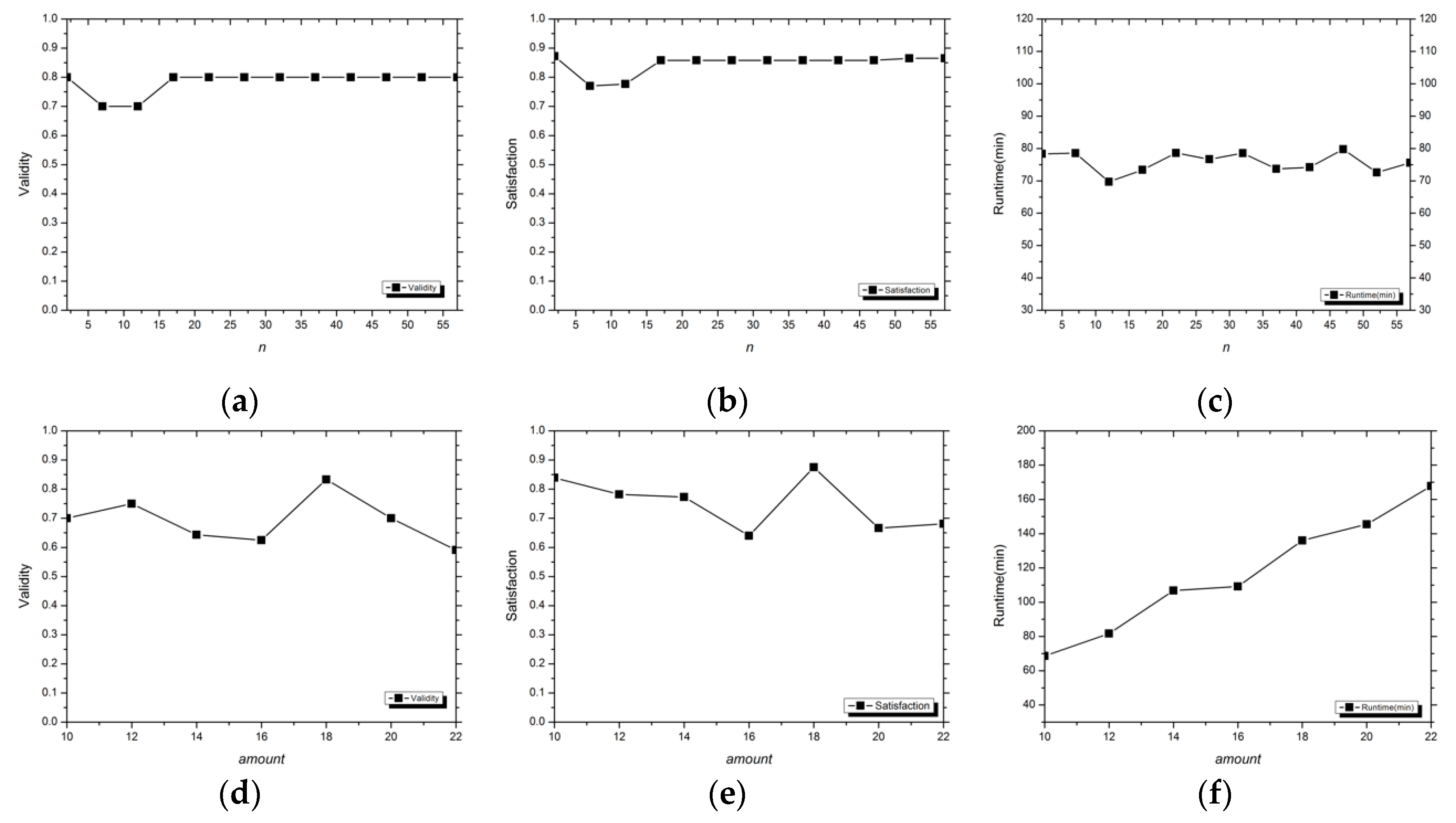
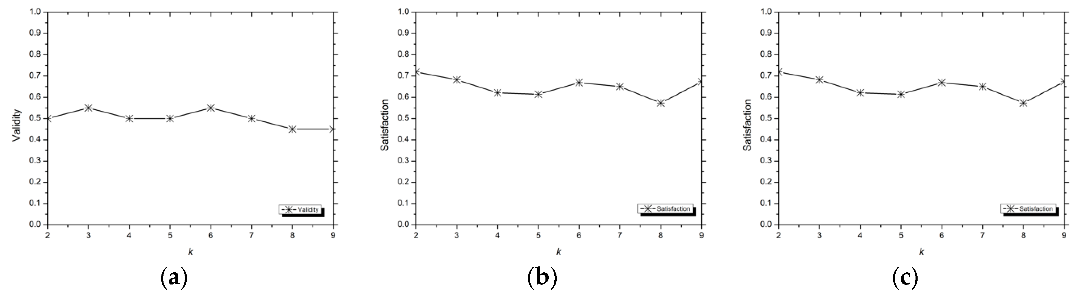
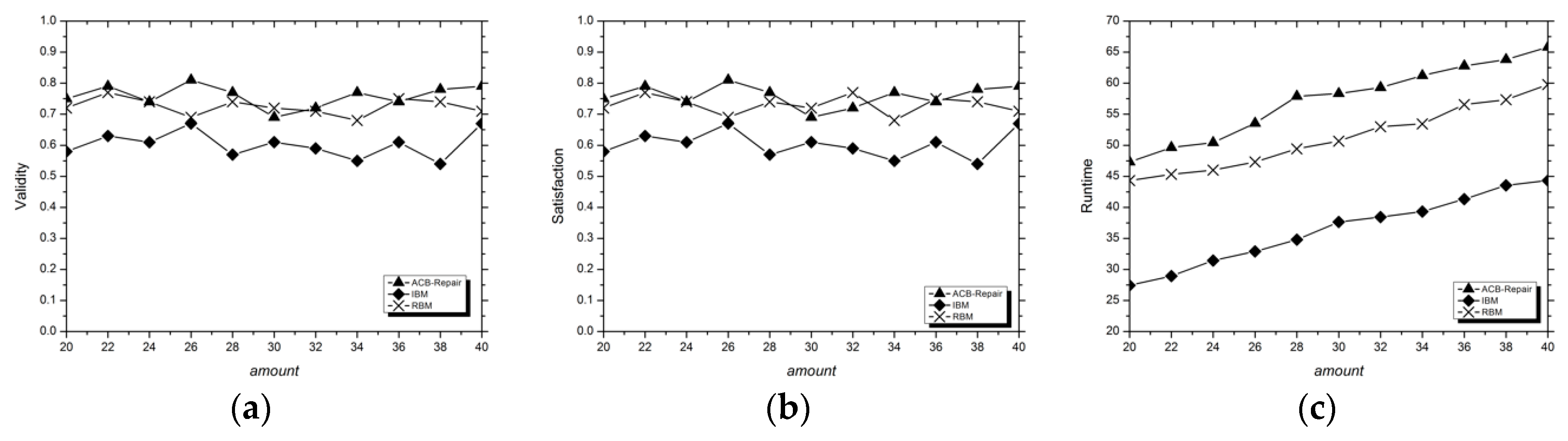
We designed three indexes—validity, satisfaction, and runtime—to evaluate the repair ability of different cleaning methods to the same erroneous data. In unsupervised data cleaning, the ACB-Repair essentially selects the most relevant elements from all data blocks as the target values of erroneous elements, so it cannot ensure all target values are the same with the corresponding initial truth values after repair. In this case, the validity, satisfaction, and runtime three indexes were adopted to measure the change in the number of erroneous elements before and after repair, the satisfaction degree between target values and the initial truth values, and the runtime of different repair processes, respectively.

Validity

The validity index was used to measure the change amount of erroneous data before and after repair, and it is described by the ratio of change amount to initial erroneous data amount. The mathematical definition is as follows.

$$\mathrm{Validity}=\frac{{{\displaystyle \sum }}_{I}su{m}_{error}-{{\displaystyle \sum }}_{I^{\prime }}su{m}_{error}}{{{\displaystyle \sum }}_{I}su{m}_{error}}$$

(18)

where the ${\displaystyle \sum }_{I}sum\_error$ and the ${\displaystyle \sum }_{I^{\prime }}sum\_error$ indicate the number of erroneous elements before and after repair, respectively.

Satisfaction

The satisfaction index is used to describe the satisfaction degree between repaired results and the truth values. In the unsupervised cleaning, different repair methods usually get different repair values, so by comparing the relative distance between repaired values and the truth values, the different repair values can be evaluated.

$$\mathrm{satisfaction}=1-\frac{{{\displaystyle \sum }}_n\frac{Dis\left(repaired,truth\right)}{max\left(repaired,truth\right)}}{n}$$

(19)

In Equation (19), the $Dis\left(repaired,truth\right)$ means the distance between repaired values and the corresponding truth values. For the numeric attributes and other attribute types, the Euclidean distance and the edit distance were adopted, respectively. The $max\left(repaired,truth\right)$ indicates the larger one between repaired values and the truth values. For the numeric attributes and other attribute types, the numeric size and string length are taken, respectively.

Runtime

The runtime index indicates the running time of the repair algorithms to erroneous elements in a given dataset. In this paper, the runtime of different repair methods is measured by the system running time.

3.2. Analysis of Experimental Results

In the MHTS dataset, we first set multiple erroneous elements amount (amount) and class-tuples amount (n) to observe the performance of the WOB-Repair (Repair without Blocking) method, which is the control group in the experiment.

First of all, we fixed the amount to 10 and kept the same EDS, the experimental results are shown in Figure 3a–c with different n.

From the results in Figure 3a–c, the n did not have a significant effect on the validity, satisfaction, and runtime indexes of the WOB-Repair method when the amount and EDS were fixed. We could even obtain exactly the same repair results from n = 17 to n = 47 (the step of n was 5), and the change of the validity index for different repair results was less than 0.1. In this case, we hold the opinion that the WOB-Repair method is stable for different n and its effect on the experimental results can be ignored. In the subsequent experiment, we chose n = 21 without explanation, when the class-tuple is 2n + 1 = 43.

Then, we fixed the n = 21 and set multiple amounts in the MHTS, the experimental results of the WOB-Repair are shown in Figure 3d–f.

Under the fixed n, the validity of the WOB-Repair fluctuated between 0.59 and 0.84, and it was stable at about 65% in the experiment. Similar to the validity index, the satisfaction of the WOB-Repair fluctuated between 0.64 and 0.88. We think it required a high repair ability in an unsupervised environment that the repair result is completely consistent with the value of the initial data set by randomly simulating the weak logic errors in the data set and comparing the repaired data set with the initial data set. From the results in Figure 3d–f, the mean validity and satisfaction of the WOB-Repair method were 65.2% and 75.1%, respectively, so that it can be effective in the unsupervised data cleaning. However, with the increase in the number of erroneous elements, the repair time of this method increases too. When the data scale is large, it takes a lot of time to clean the erroneous data through the non-blocking WOB-Repair algorithm, which may not be suitable.

The experimental results in Figure 3 were obtained by the WOB-Repair, which was the control group in the experiment, under different conditions. In the following sections, we will compare the WOB-Repair method with the ACB-Repair blocked by the RBA, SBA, and RWBA, and observe the impact of the blocking methods with different clustering accuracies on the data repair. In order to describe conveniently and distinguish different blocking methods, we used the RBA, SBA, and RWBA to express the ACB-Repair algorithm blocked by the corresponding method.

In the MHTS dataset, we fixed the amount to 20 and with both the same EDS and n as the WOB-Repair, and the experimental results of the RBA method are shown in Figure 4 by setting multiple blocking amounts (k).

The results of the RBA in Figure 4 were obtained in the same environment (amount, EDS, and n) as the WOB-Repair, and the blocking amount determined the tuple amount of a data block when blocking. In the experiment, the runtime of the RBA decreased obviously and the validity decreased slowly, while the satisfaction remained relatively stable, as data blocks increased. Combining the experimental results in Figure 3 and Figure 4, although the RBA can significantly reduce the runtime of the repair process, its repair results were not satisfactory compared to the WOB-Repair. For example, when k = 2, the runtime of the RBA decreased from the 145.49 minutes of the WOB-Repair to 46.49 minutes, but the validity and satisfaction changed from the 0.7 and 0.666 of the WOB-Repair to 0.5 and 0.719, respectively. We think validity is more important than satisfaction when evaluating the repair ability of different methods because it directly measures the change in the number of erroneous elements before and after repair. In this case, although the satisfaction of the RBA at k = 2 was higher than the WOB-Repair, we still regard the WOB-Repair as having better repair ability.

Different from the RBA, the SBA takes the Jaccard similarity among tuples to cluster and block. In the MHTS dataset, we fixed the amount to 20 and with both the same EDS and n as the WOB-Repair and RBA, and the experimental results of the SBA method are shown in Figure 5 by setting multiple matching determination thresholds ($th{d}_s$). During the experiment, we found that when the $th{d}_s$ was small, the tuple amounts of the first few blocks were very large, which made other blocks contain fewer tuples. In order to control the size of the data blocks, we set all tuple amounts to not exceed n/2 (n is the tuple amount of $I_{cf}$).

From the results in Figure 5a, the validity of the SBA method is affected to some extent by the $th{d}_s$. When the $th{d}_s$ is small, the SBA has good repair results, and its validity is stable at a low level with the increase of the $th{d}_s$. In Figure 5b,c, the satisfaction of the SBA fluctuates, and has no obvious variation tendency, but the runtime of this method decreases significantly. We think this is mainly because the larger $th{d}_s$ always divides the $I_{cf}$ into more data blocks, which makes the tuple amount in a data block smaller, thus reducing the runtime of the method.

The $th{d}_s$ in the SBA method could reflect the similarities among tuples in data blocks, and the bigger $th{d}_s$ meant better clustering accuracy. In the experiment, we found that too big a $th{d}_s$ can make the validity index of the SBA method decrease sharply. For example, when the $th{d}_s$ = 0.36, the validity = 0.65, but when the $th{d}_s$ = 0.51, the corresponding validity = 0.45. We guess this phenomenon may be caused by the following two reasons. (1) The bigger $th{d}_s$ reduces the tuple amounts of some data blocks, and the tuple amount can affect the validity of methods, thus weakening the repair ability of the SBA. (2) The bigger $th{d}_s$ increases the clustering accuracy of data blocking, and higher clustering accuracy will aggregate tuples with the same values, which may reduce the validity of the SBA method. In order to verify the viewpoint (2), we adopted the RWBA method with higher clustering accuracy to carry out subsequent experiments.

The RWBA obtains the structural information in a similarity graph by random walk with restart, and it considers not only the direct correlation among tuples but also their indirect correlation through other tuples when blocking. In the MHTS dataset, we fixed the amount to 20 and with both the same EDS and n as the WOB-Repair, RBA, and SBA, and the experimental results of the RWBA method are shown in Figure 6 by setting multiple thresholds ($th{d}_r$). Because we normalized the columns of the convergent state vector ${\pi }_{\ast }$, and the tuple amount of $I_{cf}$ was 1240, we set the multiple $th{d}_r$ as $5\ast {10}^{-4}$,$5.5\ast {10}^{-4}$,…,$8.5\ast {10}^{-4}$,$9\ast {10}^{-4}$.

Similar to the analysis in Section 2.2.2, the RWBA had a very high time complexity when the tuple amount of $I_{cf}$ was large, which mainly manifests in computing all similarity pairs and the iteration on a similarity graph. For example, when the tuple amount of $I_{cf}$ was 1240, it took 22.97 hours to establish the similarity graph for the RWBA, which contains 768,180 similarity pairs, under the experimental environment in Section 3.1.1. We found the runtime of the RWBA was much longer than the WOB-Repair, RBA, and SBA methods. In this case, we no longer payed attention to the runtime index of the RWBA, but focused on the analysis of its validity and satisfaction indexes. In Figure 6c, with the increase of the $th{d}_r$, the blocking amount of the RWBA increased gradually too. However, unlike the SBA method, its validity and satisfaction indexes were relatively stable unexpectedly, and were not significantly affected by the tuple amount of blocks. We think this may be attributed to the random walk with restart process, which enabled the RWBA to learn the correlation more accurately from a small data block. During the experiment, although the results obtained by the RWBA were more stable than the SBA method, the mean and peak value of its validity were only 0.54 and 0.55, respectively, which were lower than those obtained by the SBA. Therefore, we believe that a blocking method with a too high clustering accuracy will reduce the repair ability in the same experimental environment.

In order to evaluate the repair ability of the three different blocking methods with the same EDS, we compared their performances on the three indexes with the same blocking amount and experimental environment. The results are shown in Figure 7.

From the experimental results, although there is little difference in the satisfaction of the WOB-Repair, RBA, SBA, and RWBA methods, the validity of the WOB-Repair was always better than the other three. In this case, we believe that the blocking methods can significantly reduce the original repair time, but the repair ability will also be reduced to a certain extent. When the blocking amount is small ($k\le 4$, where the mean of the tuple amount was 310 in the experiment), the SBA had better repair results compared with the RBA and RWBA. With the increase in the k, the tuple amounts in the blocks decreased gradually. For example, when the k = 2, the smallest data block of the RWBA contains 558 tuples, but when k = 9, the largest data block of the RWBA only contains 229 tuples, under these conditions, the validity of the SBA decreases most obviously, and the RWBA performs most stably and it can still maintain relatively better repair ability than the RBA and SBA when the tuple amounts of blocks are small.

Although the RWBA has the most stable repair results in small data blocks, it has a very high time complexity when data scale is large, and the time to establish a similarity graph for $I_{cf}$ is even far longer than the WOB-Repair method. In actual repair processes, we can control the blocking amount by controlling the size of $th{d}_s$, so as to ensure the repair ability of the SBA. Therefore, we regard that the SBA has the best repair ability combining the validity, satisfaction, and runtime of the three indexes.

Then, we compared the RBM and IBM methods with the ACB-Repair blocked by the SBA on the TCC dataset. In the TCC dataset, we set the matching determination thresholds of SBA ($th{d}_s$) to 0.36 and there were multiple erroneous data amounts (amount). The validity, satisfaction, and runtime indexes of the RBM, IBM, and ACB-Repair are shown in Figure 8.

From the experimental results, we can see that the ACB-Repair based on similarity blocking methods performed best in the validity index for the same erroneous data in the TCC dataset, but because of the existence of the learning processes, the repair runtime was also the longest. The RBM method had little difference in the satisfaction index with the ACB-Repair, but its repair validity was slightly lower than the ACB-Repair method, and its runtime was also shorter. In view of the IBM method, although it had a fast repair speed, it was inferior to the previous two methods on the validity or satisfaction indexes. For the erroneous data in the datasets, we hold the opinion that the validity index can directly measure the change in the number of erroneous elements before and after repair so that it may be more important. Furthermore, we guess the reason why the RBM and IBM, especially the IBM method, perform relatively badly in the TCC dataset is that they tend to synthesize a new repair value based on existing values in the dataset rather than selecting the most relevant value to repair. In this case, their repair values may never appear in the given dataset, so these methods may be difficult to adapt to unsupervised scenarios. In summary, we think ACB-Repair is effective in unsupervised data cleaning.

4. Discussion

For weak logic errors in unsupervised data cleaning, we proposed an attribute correlation-based (ACB-Framework) under blocking, which learns the attribute correlation from all data blocks through the machine learning method with symmetric uncertainty, and computes the weighted distances between the tuple of the erroneous data and other tuples in every data block according to the learning correlation to repair. In order to reduce the time cost, we designed three different blocking methods to test the impact of clustering accuracy on the repair process. From the experimental results in Section 3.2, we found that although the blocking methods had worse repair abilities than the method without blocking, the repair time could be significantly reduced. In some fields where the real-time requirements for data cleaning are high, such as internet pages, network servers, and sensor information acquisition, we allow reducing the repair ability within a certain range to improve its real-time performance, which makes the ACB-Framework applicable.

In the experiment, when the tuple amounts of data blocks are large (i.e., the blocking amount is small), the SBA has the best repair results among the three blocking methods, and when the tuple amounts are small, the RWBA gets the best and the most stable repair results. We think this may be attributed to the random walk with restart process, which computes the convergence state on a similarity graph to obtain the indirect correlation transmitted by other tuples. However, when the original data scale is tremendous, it has a very high time complexity to establish the similarity graph and compute the convergence state for the RWBA, even exceeding the WOB-Repair method, which makes the applicability of the RWBA very poor. Although the RWBA method has the best clustering accuracy and its repair ability is not significantly affected by the tuple amounts of blocks compared with the RBA and SBA methods, its mean and peak value of the repair validity is inferior to the SBA when tuple amounts of blocks are large. Therefore, we think that a too high clustering accuracy will agglomerate more tuples with the same elements, which can reduce repair validity. For the problem, the SBA performed poorly in data blocks with fewer tuples. We can control the tuple amount by controlling the size of $th{d}_s$ in applications, so as to ensure its repair ability. Furthermore, we compared the optimal threshold of the SBA method in the previous experiment with the two methods of RBM and IBM to verify the effectiveness of our proposed method.

However, although the RBA and SBA methods can reduce the repair time, their repair results for the erroneous data were both worse than the WOB-Repair method without blocking. In this case, how to maintain the repair abilities of methods on the basis of reducing their repair time is a question worth considering. The subsequent research will explore the following two aspects:

(1)

How to design better repair methods in unsupervised data cleaning?

(2)

How to further reduce the cleaning time while better maintaining its cleaning ability?

5. Conclusions

The main achievement of this paper was the division of data cleaning into the supervised and unsupervised forms according to whether there were interventions in the repair processes. Due to the lack of sufficient domain knowledge to guide repair under the unsupervised environment, we hold the opinion that multiple data quality problems with different traditional dimensions can be repaired by similar methods, and propose a new dimension suitable for unsupervised cleaning. In view of weak logic errors in unsupervised data cleaning, we propose an attribute correlation-based framework under blocking to repair them, and designed three different data blocking methods to reduce the time complexity and test the impact of clustering accuracy on data cleaning. From the experimental results, although the blocking methods may reduce the repair ability to a certain extent, they can greatly reduce the repair time. Moreover, the ACB-Framework does not need the guidance of domain knowledge and interventions in the repair process, in some fields with large data scales, frequent data updating, and high real-time requirements, it can have certain application value.

References

- Wang, H.Z.; Li, M.D.; Bu, Y.Y.; Li, J.Z.; Gao, H.; Zhang, J.C. Cleanix: A Parallel Big Data Cleaning System. SIGMOD Rec. 2015, 44, 35–40. [Google Scholar] [CrossRef]
- Xu, S.; Lu, B.; Baldea, M.; Edgar, T.F.; Wojsznis, W.; Blevins, T.; Nixon, M. Data cleaning in the process industries. Rev. Chem. Eng. 2015, 31, 453–490. [Google Scholar] [CrossRef]
- Liu, X.L.; Li, J.Z. Consistent Estimation of Query Result in Inconsistent Data. Chin. J. Comput. 2015, 9, 1727–1738. [Google Scholar]
- Fujii, T.; Ito, H.; Miyoshi, S. Statistical-Mechanical Analysis Connecting Supervised Learning and Semi-Supervised Learning. J. Phys. Soc. Jpn. 2017, 86, 6. [Google Scholar] [CrossRef]
- Fabris, F.; de Magalhes, J.P.; Freitas, A.A. A review of supervised machine learning applied to ageing research. Biogerontology 2017, 18, 171–188. [Google Scholar] [CrossRef]
- Xu, S.L.; Wang, J.H. Classification Algorithm Combined with Unsupervised Learning for Data Stream. Pattern Recognit. Artif. Intell. 2016, 29, 665–667. [Google Scholar]
- Kim, J.; Jang, G.J.; Lee, M. Investigation of the Efficiency of Unsupervised Learning for Multi-task Classification in Convolutional Neural Network. In Proceedings of the International Conference on Neural Information Processing, Kyoto, Japan, 16–21 October 2016; pp. 547–554. [Google Scholar]
- Can, B.; Manandhar, S. Methods and Algorithms for Unsupervised Learning of Morphology. In Proceedings of the International Conference on Intelligent Text Processing and Computational, Kathmandu, Nepal, 6–12 April 2014; pp. 177–205. [Google Scholar]
- Zhou, J.L.; Diao, X.C.; Cao, J.J.; Pan, Z.S. An Optimization Strategy for CFDMiner: An Algorithm of Discovering Constant Conditional Functional Dependencies. IEICE Trans. Inf. Syst. 2016, E99.D, 537–540. [Google Scholar] [CrossRef]
- Li, M.H.; Li, J.Z.; Cheng, S.Y.; Sun, Y.B. Uncertain Rule Based Method for Determining Data Currency. IEICE Trans. Inf. Syst. 2018, E101-D, 2447–2457. [Google Scholar] [CrossRef]
- Mcgilvray, D. Executing Data Quality Projects; Elsevier LTD Press: Oxford, UK, 2008. [Google Scholar]
- Zhang, L.; Zhao, Y.; Zhu, Z.F.; Shen, D.G.; Ji, S.W. Multi-View Missing Data Completion. IEEE Trans. Knowl. Data Eng. 2018, 30, 1296–1309. [Google Scholar] [CrossRef]
- Diao, Y.L.; Sheng, W.X.; Liu, K.Y.; He, K.Y.; Meng, X.L. Research on Online Cleaning and Repair Methods of Large-Scale Distribution Network Load Data. Power Syst. Technol. 2015, 11, 3134–3140. [Google Scholar]
- Benbernou, S.; Ouziri, M. Enhancing Data Quality by Cleaning Inconsistent Big RDF Data. In Proceedings of the 2017 IEEE International Conference on Big Data (Big Data), Boston, MA, USA, 11–14 December 2017; pp. 74–79. [Google Scholar]
- Fisher, J.; Christen, P.; Wang, Q.; Rahm, E. A Clustering-Based Framework to Control Block Sizes for Entity Resolution. In Proceedings of the 21th ACM SIGKDD International Conference on Knowledge Discovery and Data Mining, Sydney, Australia, 10–13 August 2015; pp. 279–288. [Google Scholar]
- Ahmad, H.A.; Wang, H. An effective weighted rule-based method for entity resolution. Distrib. Parallel Databases 2018, 36, 593–612. [Google Scholar] [CrossRef]
- Wang, H.Z.; Li, J.Z.; Gao, H. Efficient entity resolution based on subgraph cohesion. Knowl. Inf. Syst. 2016, 46, 285–314. [Google Scholar] [CrossRef]
- Brisaboa, N.R.; Rodriguez, M.A.; Seco, D.; Troncoso, R.A. Rank-based strategies for cleaning inconsistent spatial databases. Int. J. Geogr. Inf. Sci. 2015, 29, 280–304. [Google Scholar] [CrossRef]
- Xu, Y.L.; Li, Z.H.; Chen, Q.; Zhong, P. Repairing Inconsistent Relational Data Based on Possible World Model. J. Softw. 2016, 27, 1685–1699. [Google Scholar]
- Martin, D.; Rosete, A.; Alcala-Fdez, J.; Herrera, F. A New Multiobjective Evolutionary Algorithm for Mining a Reduced Set of Interesting Positive and Negative Quantitative Association Rules. IEEE Trans. Evol. Comput. 2014, 18, 54–69. [Google Scholar] [CrossRef]
- Perez-Alonso, A.; Medina, I.J.B.; Gonzalez-Gonzalez, L.M.; Chica, J.M.S. Incremental maintenance of discovered association rules and approximate dependencies. Int. Data Anal. 2017, 21, 117–133. [Google Scholar] [CrossRef]
- Zhang, X.J.; Wang, M.; Meng, X.F. An Accurate Method for Mining top-k Frequent Pattern under Differential Privacy. J. Comput. Res. Dev. 2014, 51, 104–114. [Google Scholar]
- Zhang, C.S.; Diao, Y.F. Conditional Functional Dependency Discovery and Data Repair Based on Decision Tree. In Proceedings of the 2015 12th International Conference on Fuzzy Systems and Knowledge Discovery (FSKD), Zhangjiajie, China, 15–17 August 2015; pp. 864–868. [Google Scholar]
- Yadav, M.L.; Roychoudhury, B. Handling missing values: A study of popular imputation packages in R. Knowl.-Based Syst. 2018, 160, 104–118. [Google Scholar] [CrossRef]
- Krishnan, S.; Franklin, M.J.; Goldberg, K.; Wu, E. Boostclean: Automated error detection and repair for machine learning. arXiv 2017, arXiv:1711.01299. [Google Scholar]
- Li, L.; Hanson, T.E. A Bayesian semiparametric regression model for reliability data using effective age. Comput. Stat. Data Anal. 2014, 73, 177–188. [Google Scholar] [CrossRef]
- Karakasidis, A.; Koloniari, G.; Verykios, V.S. Scalable Blocking for Privacy Preserving Record Linkage. In Proceedings of the 21th ACM SIGKDD International Conference on Knowledge Discovery and Data Mining, Sydney, Australia, 10–13 August 2015; pp. 527–536. [Google Scholar]
- Papadakis, G.; Papastefanatos, G.; Koutrika, G. Supervised Meta-blocking. Proc. VLDB Endow. 2014, 7, 1929–1940. [Google Scholar] [CrossRef]
- Kim, J.S.; Sim, J.Y.; Kim, C.S. Multiscale Saliency Detection Using Random Walk with Restart. IEEE Trans. Circuits Syst. Video Technol. 2014, 24, 198–210. [Google Scholar]
- Sun, C.C.; Shen, D.R.; Kou, Y.; Nie, T.Z.; Yu, G. Entity Resolution Oriented Clustering Algorithm. J. Softw. 2016, 27, 2303–2319. [Google Scholar]
- Tong, H.H.; Faloutsos, C.; Pan, J.Y. Fast random walk with restart and its applications. In Proceedings of the Sixth International Conference on Data Mining, Hong Kong, China, 18–22 December 2006. [Google Scholar]
- Le, H.T.; Urruty, T.; Gbehounou, S.; Lecellier, F.; Martinet, J.; Fernandez-Maloigne, C. Improving retrieval framework using information gain models. Signal Image Video Process. 2017, 11, 309–316. [Google Scholar] [CrossRef]
- Ye, M.Q.; Gao, L.Y.; Wu, C.R.; Wan, C.Y. Informative Gene Selection Method Based on Symmetric Uncertainty and SVM Recursive Feature Elimination. Pattern Recognit. Artif. Intell. 2017, 30, 429–438. [Google Scholar]