Fractional-Order Fusion Model for Low-Light Image Enhancement

Abstract

In this paper, a novel fractional-order fusion model (FFM) is presented for low-light image enhancement. Existing image enhancement methods don’t adequately extract contents from low-light areas, suppress noise, and preserve naturalness. To solve these problems, the main contributions of this paper are using fractional-order mask and the fusion framework to enhance the low-light image. Firstly, the fractional mask is utilized to extract illumination from the input image. Secondly, image exposure adjusts to visible the dark regions. Finally, the fusion approach adopts the extracting of more hidden contents from dim areas. Depending on the experimental results, the fractional-order differential is much better for preserving the visual appearance as compared to traditional integer-order methods. The FFM works well for images having complex or normal low-light conditions. It also shows a trade-off among contrast improvement, detail enhancement, and preservation of the natural feel of the image. Experimental results reveal that the proposed model achieves promising results, and extracts more invisible contents in dark areas. The qualitative and quantitative comparison of several recent and advance state-of-the-art algorithms shows that the proposed model is robust and efficient.

1. Introduction

Primarily, people receive information daily in the form of audio and images.The human mind interprets and processes visual information efficiently. The images captured with digital devices may be influenced by various conditions such as bad light, weather, noise, etc. The low illumination images have different forms such as one side dark and one side bright or some particular portion effect with bad light. Hence, it is difficult for the human eye to extract hidden meaningful contents from these images. Currently, the enhancement techniques used for images degraded from various conditions have a wide range of applications and significant impact on the performance of various high-precision computer vision systems, such as target tracking [1], object detection [2], and medical image analysis [3].

There are numerous algorithms that have been proposed to make visible the hidden contents. The simplest method Histogram Equalization (HE) [4,5] solves this problem by equalizing the histogram of the original image. The disadvantage of this method is that it enhances the contrast and don’t pay attention to real illumination cases. The results are always super-saturated or over-enhanced. According to the observations, the inversion of low-light images is close to hazy images. The technique in [6,7] transforms the original images into a photo-negative effect and uses the dehaze strategy to enhance. However, those methods cause the results look unnatural due to the lack of physical theory support. The most widely used theory for image enhancement is the Retinex theory (RT) [8]. Based on this theory, an image can be viewed as the product of reflectance and illumination [8]. Retinex-based methods use a variety of priors to get illumination, and then adjust the illumination to enhance the low-light images [9,10,11,12]. Naturalness preserved enhancement (NPE) [12] uses a bright-pass filter to decompose the original image into illumination and reflectance. Cai et al. [9] introduced a model that constrains illumination and reflection by shape, texture and illumination priors. The objective assessment of this method is good, but the results are still dark. Based on the Retinex methods, Fu et al. [13] use arc tangent transformation and histogram equalization to adjust the illumination, and then the two type weights are used to fuse these adjusted illuminations. However, the enhanced images have the risk of over-exposure due to the inclusion of the histogram equalization method. Ying et al. [11] propose a Camera Response Model (CRM) to make the adjusted illumination more similar to camera exposure. This is the era of neural networks, and different neural network methods [14,15,16,17] have emerged. Li et al. [17] use a Convolutional Neural Network to predict the good exposure illumination map. However, the processed images have visible visual artifacts.

Although there are many algorithms that process and extract hidden contents in low-light images, still there are several problems that should be solved. The existing algorithms may not fully extract the dark contents from the original image, which can’t get good visual effects in low illumination regions, and have the risk of over-enhancement. We proposed a fractional-order fusion model to enhance images well and solve all the problems. Firstly, fractional-order is used to preserve the naturalness of the original image. Secondly, traditional methods use gamma transformation for illumination adjustment, but the processed image is a bit distorted due to lack of physical theory support [11]. Inspired by [11], the illumination adjustment strategy suitable for this model is applied to get the desired results. Finally, the proposed model extracts more contents in the low light region by using the fusion framework. An intuitive idea for extracting more contents is to treat the enhanced images as pending images and process it again. However, the error of pixel value in the low-light areas may be magnified, and affect the quality of results. To solve this issue, the proposed model process images with a denoising strategy before the second image enhancement step, as shown in Figure 1. After the second image enhancement step, the fusion process is applied to compensate for the loss of detail due to the filtering while improving image brightness and avoiding over-enhancement.

Contribution: The main contributions of the proposed model are:

• As compared to integer-order, we apply fractional calculus to process the original images without logarithmic transformation. Remarkable results have been achieved in preserving the natural character of images.
• A novel fusion framework is introduced to extract more contents in the dark areas while preserving the visual appearance of images.
• The experimental results compared with other image enhancement algorithms show that the proposed model can reveal more hidden contents in dark regions of the images.

This paper is structured as follows: Section 2 is a brief introduction to fractional calculus and Retinex theory. The proposed model is elaborated in detail in Section 3. Section 4 describes the implementation of the algorithm. The qualitative and quantitative analysis is in Section 5, and Section 6 is related to the conclusions and future work.

2. Background

In this section, we introduce the fractional calculus and the Retinex theory briefly.

2.1. Fractional Calculus

Fractional calculus was born in 1695, almost as long as classic calculus. Fractional calculus is widely used in signal processing and image processing because of its strength such as long-term memory, weak singularity, and non-locality [18,19,20]. The most commonly used fractional calculus definitions are Grünwald-Letnikov, Riemann–Liouville, and Caputo [21,22,23]. The Grünwald-Letnikov definition is used as follows:

$$\begin{array}{c}\hfill {}_a^{G-L}{D}_x^{v}f(x)=\underset{N\to \infty }{\lim }\{\frac{{(\frac{x-a}{N})}^{-v}}{\Gamma (-v)}\sum _{k=0}^{N-1}\frac{\Gamma (k-v)}{\Gamma (k+1)}·f(x-k(\frac{x-a}{N}))\},\end{array}$$

(1)

where $[a,x]$ is the domain of $f(x)$, and v is an arbitrary number which indicates the order of the derivation. $\Gamma (\alpha )={\int }_0^{\infty }{e}^{-x}{x}^{\alpha -1}dx$ is the gamma function.

2.2. Retinex Theory

The Retinex theory (RT) [8] is proposed by Edwin Land to explain human color vision system. The basic formula of Retinex is as follows:

$$S=R·L,$$

(2)

where S is the observed image. R reflectance and L is illumination, respectively. The reflectance represents the intrinsic characteristics of the object, and the illumination represents the extrinsic property. · indicates element-wise multiplication. Furthermore, RT has been used with slight modification to achieve good quality results [24].

The previously proposed fractional-order models [25] processed the log-transformed image, i.e., $s=r+l$ where s, r and l are $log(S)$, $log(R)$ and $log(L),$ respectively. However, it is not appropriate to process the log-transformed image according to [26]. The important textures and edges in high magnitude stimuli areas may be masked by noise and irrelevant details in low illumination areas when taking the derivative. It is because $▽log(x)=\frac{1}{x}▽x$, when x is very small, the weight of $▽x$ will be very large, $▽log(x)$ is highly affected by $\frac{1}{x}$. This problem is solved in this paper by processing the original image directly.

The Retinex-based algorithms get L and R from S through various priors, and then adjust L and R to get the final enhanced results.

3. Fractional-Order Fusion Model Based On Retinex

In this section, we present the step by step explanation of the proposed model. The model steps are:

3.1. Reflectance and Illumination Based On Fractional-Order

3.1.1. Reflectance

According to [12], the reflectance is piece-wise continuous and contains fine textures. The traditional methods use integer-order differential to constrain reflectance, such as $\Vert D_{x/y}R{\Vert }_1$, $\parallel D_{x/y}{R\parallel }_2^2$. However, using fractional calculus gets better effects on preserving texture details and suppressing noise according to Section 5.1. The energy function is modeled as:

$$E_r(R)=\parallel {(D_x^{v1}R)}^{v2}{\parallel }_1+{\parallel {(D_y^{v1}R)}^{v2}\parallel }_1,$$

(3)

where ${\parallel •\parallel }_1$ designates $l_1$ norms, and $v1$, $v2$ are fractional parameters.

3.1.2. Illumination

The detailed information about the illumination priors are as follows:

• For color images, three color channels (R, G, B) share the same illumination map [27].
• R is restricted to the unit interval, according to Equation (2), we know $S\le L$.
• L and S should be close enough [10].
• L should contain the structural information of the image and remove the texture details [9,27].

To express the information shown in 1, 2, 3, we can design the formula as:

$$\Vert L-\widehat{L}{\Vert }_2^2,$$

(4)

where ${\parallel •\parallel }_2$ designates $l_2$ norms, and $\widehat{L}$ is the initial illumination map.

$$\widehat{L}(x)=\underset{y\in \mathrm{\Omega }(x)}{\max }\underset{c\in \{R,G,B\}}{\max }{S}^c(y),$$

(5)

where x is the pixel of interest. $\mathrm{\Omega }(x)$ donates the pixels’ neighboring x. c represents three color channels.

The 4th illumination prior indicates that we should simultaneously preserve the overall structure and smooth the textural details. The proposed illumination constraint is:

$$E_l(L)={∥\frac{D_{x}L}{D_{x}G(L)+ϵ}∥}_1+{∥\frac{D_{y}L}{D_{y}G(L)+ϵ}∥}_1,$$

(6)

where $ϵ$ is a small number to avoid division by zero. $G(•)$ means Gaussian filtering. In the texture detail areas, $|D_{x/y}G(L)|$ is small compared to $|D_{x/y}L|$. This is because Gaussian filtering leads to loss of details in these areas, so $E_l(L)\gg 2$. In the structural detail areas, the patch around L changes in accordance, $|D_{x/y}G(L)|$ and $|D_{x/y}L|$ are very close, so $E_l(L)\approx 2$.

3.1.3. The Energy Function

The total energy function can be obtained by combining the illumination priors, reflection priors, and the fidelity term. The optimization goal is as follows:

$$E_s(L,R)={\parallel L·R-S\parallel }_2^2+\alpha E_l(L)+\beta E_r(R)+\lambda \Vert L-\widehat{L}{\Vert }_2^2,$$

(7)

where $\alpha$, $\beta$, and $\lambda$ are the coefficients to balance the involved four terms. The fidelity term ${\parallel L·R-S\parallel }_2^2$ is to ensure that the image ($L·R$) and the original image are very close. By solving $\underset{R,L}{\min }{E}_s(L,R)$, we can get L and R that match our priors.

3.1.4. Adjust Illumination

Once the reflectance (R) and illumination (L) are solved, the next step is to adjust illumination. Traditional methods use gamma transformation to adjust illumination. The equation is defined as:

$$S^{\prime }=I^{\prime }·R=I^{\frac{1}{\gamma }}·R,$$

(8)

where $S^{\prime }$ is the enhanced image, $I^{\prime }$ is the adjusted illuminate and $\gamma$ is the empirical parameter, $\gamma =2.2$ in general.

Recently, Ying et al. [11] proposed camera response function (CRF) to adjust illumination, which is inspired by the response characteristics of cameras. The equation is defined as:

$$g(\mathbf{P},k)=\beta {\mathbf{P}}^{\gamma }=e^{b(1-k^a)}{\mathbf{P}}^{(k^a)},$$

(9)

where k is exposure ratio, and $k=1\oslash L$. $\mathbf{P}$ is the input image, and g is enhanced image; a and b are constants, $a=-0.3293$ and $b=1.1258$.

Since the prior conditions of the proposed model are different from [11], parameters a and b shouldn’t apply to the proposed model directly. As shown in Figure 2, (a) and (e) are a pair of images that differ only in exposure. (b) and (c) are the results of the gamma transformation and the original CRF, respectively. The result of Gamma transformation is a bit dim, and the original CRF produces the over-saturated effect.

In order to set the enhancement process to present the images as close as possible to the well-exposure image, we adjust the parameters a and b, and then set the histogram of them as consistent as possible. Finally, the appropriate parameters are found, $a=-0.2195$ and $b=1.1258$. The final result is shown in Figure 2d.

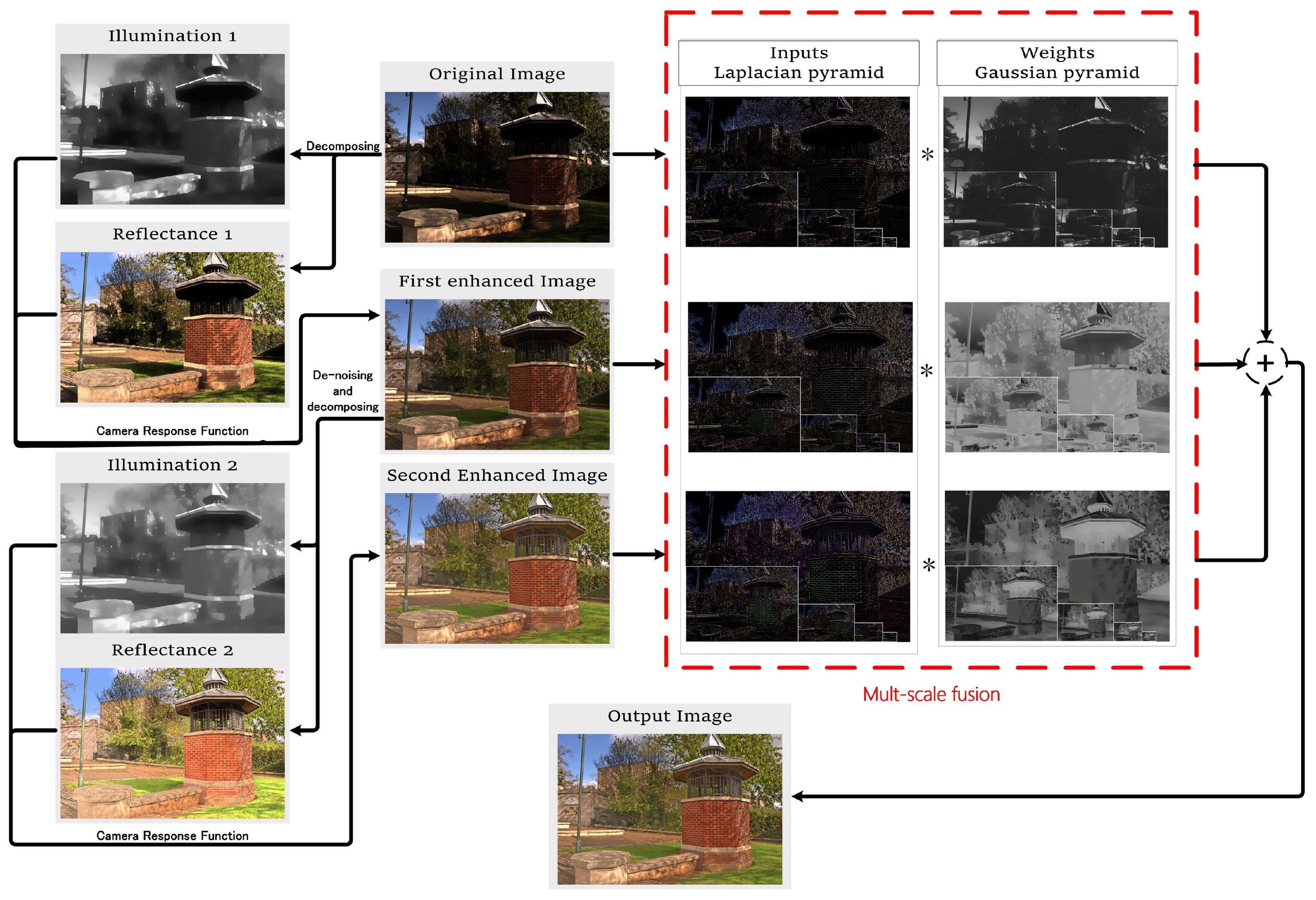
3.2. Fusion Framework

In the general Retinex-based algorithms, the final step is to adjust the illumination and get an enhanced result. However, the contents of low-light images may not be fully revealed. Therefore, a fusion method is proposed to extract more hidden contents.

As shown in Figure 1, firstly, the input image is divided into R and L using Equation (7), and CRF is applied to adjust exposure. Secondly, in order to extract more contents while preserving visual quality, BM3D [28] is used to filter the first enhanced image, and then another enhancement is made to the result. Finally, the fusion process is applied to get the final enhance result.

The fusion framework can be expressed as the following formula:

$$\mathbf{J}(x,y)=\sum _{i=1}^k{\mathbf{W}}_i(x,y)f({\mathbf{E}}_i(x,y)),$$

(10)

where ${\mathbf{W}}_i$ is the weight of the i-th image, and ${\sum }_{i=1}^k{\mathbf{W}}_i(x,y)=1$. In the proposed model, $k=3$, ${\mathbf{E}}_1$, ${\mathbf{E}}_2$ and ${\mathbf{E}}_3$ denote the original image, first enhanced image and second enhanced image, respectively. $\mathbf{J}$ donates the final result.

As showing in Figure 3, (a), (b) and (c) are ${\mathbf{E}}_1$, ${\mathbf{E}}_2$ and ${\mathbf{E}}_3$, respectively. For ${\mathbf{E}}_1$, it is ideal to enhance the areas with low illumination, while retaining the areas with high illumination. On the contrary, ${\mathbf{E}}_3$ has a serious loss of details due to the filtering process, and it can reveal more contents compared with (a) and (b), it is ideal to retain the areas with low illumination. It is similar to supervised machine learning. Therefore, the sigmoid function widely used in machine learning is used to set the weights of ${\mathbf{E}}_1$ and ${\mathbf{E}}_3$. According to [13], the pixel distribution of well-exposed images approximates Gaussian distribution with a mean of 0.5 and a variance of 0.25. The weight of ${\mathbf{E}}_2$ is set to the Gaussian function. In order to balance the Gaussian distribution function and Sigmoid, several changes are made to the standard formulas and get the following weight formulas:

$$\begin{array}{c}{\mathbf{W}}_1=\frac{1}{1+e^{-4I_1+2}},\end{array}$$

(11)

$$\begin{array}{c}{\mathbf{W}}_2=e^{-\frac{1}{2}\frac{{(I_2-0.5)}^2}{{0.25}^2}},\end{array}$$

(12)

$$\begin{array}{c}{\mathbf{W}}_3=\frac{1}{1+e^{4I_3-2}},\end{array}$$

(13)

where I is the corresponding illumination. The normalization process is performed after calculating the weights by illumination.

As can be seen from Figure 3e, ${\mathbf{E}}_1$ dominates where the illumination is strong, ${\mathbf{E}}_2$ has a large weight around 0.5, and ${\mathbf{E}}_3$ dominates in areas with dark light. The result, Figure 3d, is brighter than ${\mathbf{E}}_1$ and ${\mathbf{E}}_2$, darker than ${\mathbf{E}}_3$. The fusion framework achieves a good balance between enhancing brightness and avoiding over-exposure.

4. Implementation of FFM

This section describes the implementation steps of the algorithm in detail.

4.1. Optimization of the Energy Function

As discussed in Section 3.1, L and R are obtained by minimizing $E_s(L,R)$. According to [29], the block coordinate descent method is adopted to minimize the energy function Equation (7). The optimal solution can be obtained by iteratively updating one variable at a time, while other parameters are treated as constants. Once all the variables converge, we get the optimal solution.

In the n-th iteration, the problem is divided into R and L sub-problems.

4.1.1. R Sub-Problem

According to [30,31], Equation (3) can be re-organized as:

$$E_r(R)=\parallel w_x·{(D_x^{v1}R)}^2{\parallel }_1+{\parallel w_y·{(D_y^{v1}R)}^2\parallel }_1,$$

$$w_x=|D_x^{v1}{R|}_{}^{v2-2},w_y={|D_y^{v1}R|}_{}^{v2-2}.$$

(14)

By ignoring items that don’t contain the variable R, we can get the energy function of R sub-problem:

$$\arg \underset{R}{\min }{\parallel L·R-S\parallel }_2^2+\beta \parallel w_x·{(D_x^{v1}R)}^2{\parallel }_1+\beta {\parallel w_y·{(D_y^{v1}R)}^2\parallel }_1.$$

(15)

This is a typical problem that can be solved by weighted least squares [32], Equation (15) can be converted into the matrix form as:

$$\begin{array}{c}\hfill \arg \underset{{\mathbf{V}}_r}{\min }{({\mathbf{V}}_l·{\mathbf{V}}_r-{\mathbf{V}}_s)}^T({\mathbf{V}}_l·{\mathbf{V}}_r-{\mathbf{V}}_s)+\beta {\mathbf{V}}_r^T{\mathbf{D}}_x^{v{1}^T}{\mathbf{W}}_x{\mathbf{D}}_x^{v1}{\mathbf{V}}_r+\beta {\mathbf{V}}_r^T{\mathbf{D}}_y^{v{1}^T}{\mathbf{W}}_y{\mathbf{D}}_y^{v1}{\mathbf{V}}_r^{},\end{array}$$

(16)

where ${\mathbf{W}}_x$ and ${\mathbf{W}}_y$ are the diagonal matrices formed by the vectorized $w_x$, $w_y$, respectively. ${\mathbf{D}}_x^{v1}$ and ${\mathbf{D}}_y^{v1}$ are the Toeplitz matrices from the discrete fractional-order gradient operators which can be obtained by Equations (A1) and (A2) (Appendix A). Since the equation is decomposed into quadratic and nonlinear parts, a numerically stable approximation can be obtained. By deriving Equation (16) and making it equal to zero, we can get the optimal solution of the n-th R:

$${\mathbf{V}}_{r_n}={({\mathbf{M}}_r+\beta {\mathbf{N}}_r)}^{-1}({\mathbf{V}}_{l_{n-1}}·{\mathbf{V}}_{s_{}}),$$

(17)

where ${\mathbf{M}}_r$ is the diagonal matrix formed by $({\mathbf{V}}_{l_n}·{\mathbf{V}}_{l_n}^{})$, ${\mathbf{N}}_r={\mathbf{D}}_x^{v{1}^T}{\mathbf{W}}_x{\mathbf{D}}_x^{v1}+{\mathbf{D}}_y^{v{1}^T}{\mathbf{W}}_y{\mathbf{D}}_y^{v1}$.

4.1.2. L Sub-Problem

It is the same as the R sub-problem, Equation (6) can re-organized as:

$$E_l(L)=\parallel u_x·{(D_{x}L)}^2{\parallel }_1+{\parallel u_y·{(D_{y}L)}^2\parallel }_1,$$

(18)

$$u_x=\frac{1}{\left|D_{x}G(L)\right||D_{x}L|+ϵ},u_y=\frac{1}{\left|D_{y}G(L)\right||D_{y}L|+ϵ}.$$

(19)

The energy function of L sub-problem can be rewritten as:

$$\arg \underset{L}{\min }{\parallel L·R-S\parallel }_2^2+\alpha \parallel u_x·{(D_{x}L)}^2{\parallel }_1+\alpha \parallel u_y·{(D_{y}L)}^2{\parallel }_1+\lambda \Vert L-\widehat{L}{\Vert }_2^2.$$

(20)

Equation (20) is transformed into the matrix form:

$$\begin{array}{c}\hfill \arg \underset{{\mathbf{V}}_l}{\min }{({\mathbf{V}}_l·{\mathbf{V}}_r-{\mathbf{V}}_s)}^T({\mathbf{V}}_l·{\mathbf{V}}_r-{\mathbf{V}}_s)+\alpha ({\mathbf{V}}_l^T{\mathbf{D}}_x^T{\mathbf{U}}_x{\mathbf{D}}_x{\mathbf{V}}_l^{}+{\mathbf{V}}_l^T{\mathbf{D}}_y^T{\mathbf{U}}_y{\mathbf{D}}_y{\mathbf{V}}_l^{})+\lambda {({\mathbf{V}}_l-{\mathbf{V}}_{\widehat{l}})}^T({\mathbf{V}}_l-{\mathbf{V}}_{\widehat{l}}).\end{array}$$

(21)

${\mathbf{V}}_l$, ${\mathbf{V}}_r$, ${\mathbf{V}}_s$ and ${\mathbf{V}}_{\widehat{l}}$ are vector forms of L, R, S and $\widehat{L}$, respectively. ${\mathbf{U}}_x$ and ${\mathbf{U}}_y$ are the diagonal matrices formed by $u_x$, $u_y$. ${\mathbf{D}}_x$ and ${\mathbf{D}}_y$ are the Toeplitz matrices from the discrete gradient operators [31]. By deriving Equation (21) and making it equal to zero, we can get the optimal solution of the n-th L:

$${\mathbf{V}}_{l_n}={({\mathbf{M}}_l+\alpha {\mathbf{N}}_l+\lambda \mathbf{1})}^{-1}({\mathbf{V}}_{r_{n-1}}·{\mathbf{V}}_{s_{}}+\lambda {\mathbf{V}}_{\widehat{l}}),$$

(22)

where ${\mathbf{M}}_l$ is the diagonal matrix formed by $({\mathbf{V}}_{r_{n-1}}·{\mathbf{V}}_{r_{n-1}}^{})$, ${\mathbf{N}}_l=({\mathbf{D}}_x^T{\mathbf{U}}_x{\mathbf{D}}_x+{\mathbf{D}}_y^T{\mathbf{U}}_y{\mathbf{D}}_y)$ and $\mathbf{1}$ is the identity matrix.

4.2. Implementation of the Fusion Process

To get the final fused result, a multi-scale fusion process is adopted. In Ref. [33], each input image processed at various scales as a sum of patterns is represented. The Gaussian kernel convolved all the inputs to produce a low-pass filtered version. To extract image features, we decompose derived inputs using the Laplacian pyramid, and to perform smooth transitions each normalized weight provides to the Gaussian pyramid. This fusion process is effective. Subsequently, it fuses image features of intensities instead. Furthermore, the use of Gaussian and Laplacian operators are well-known techniques, and one can easily implement them for practical applications. The numbers of levels are the same for both Laplacian and Gaussian pyramids.

5. Experiments and Analysis

5.1. Fractional Order Impact

Since the fractional-order reflectance prior has not been adopted in previous non-logarithmic Retinex algorithms, its impact is analyzed in this experiment. To be more intuitive to see the advantages of fractional order, we simplify the problem to a one-dimensional signal. As shown in Figure 4a, it is the original signal, the square wave represents the structure of the image, and the triangle wave represents texture details. Figure 4b shows the signal with Gaussian noise, expressed with g. It is desired to denoise and maintain the texture details of g. There are three models to solve this problem, as shown in Formula (23)–(25):

$$\underset{f}{\min }||g(x)-{f(x)\Vert }_2^2+{\lambda }_1||D_{x}f(x){\Vert }_1,$$

(23)

$$\underset{f}{\min }||g(x)-{f(x)\Vert }_2^2+{\lambda }_2||D_{x}f(x){\Vert }_2^2,$$

(24)

$$\underset{f}{\min }||g(x)-{f(x)\Vert }_2^2+{\lambda }_3||D_x^{v}f(x){\Vert }_1,$$

(25)

where the first term in Equations (23)–(25) is fidelity item, and the second item is the regularization term. ${\lambda }_1$, ${\lambda }_2$ and ${\lambda }_3$ are coefficients to balance the fidelity and regularization terms. Equations (23) and (24) are conventional methods. We use fractional differential denoise technique in Equation (25).

The experimental results are shown in Figure 4c–i clearly. According to Equation (23), the signal has lost some details but is not smooth. The model of Equation (24) has improved denoising ability. However, as ${\lambda }_2$ increases, some important details are lost. Compared with Equations (23) and (24), fractional calculus does have its unique advantages. The signal is smooth, and the details are still obvious. Therefore, the fractional order is used in Equation (3). This experiment also proves that the optimization algorithm can get good results while solving fractional-order equations.

The impact of fractional-order differential for image enhancement is shown in Figure 5. It clearly shows that the fractional-order preserves more contents in the dark area.

5.2. Comparison with Other Algorithms

To validate the performance of the proposed model, three public available datasets (MF-data [13], NPE-data [12], and Middlebury [34]) is used. The Middlebury is a multi-exposure dataset, and the relatively dark images are selected for the experiments. The NPE-data contains the three databases (NPEpart1, NPEpart2, NPEpart3). The proposed model is compared to state-of-the-art methods, such as JIEP [9], NPE [12], CRM [11], MF [13], and LightenNet [17]. Since the first enhancement of the proposed model is regarded as a Retinex-based method, the method comparison includes the first enhanced result (FFM(1)) and the final result (FFM(2)).

During the experiments, the parameters $\alpha =0.001$, $\beta =0.05$ and $\lambda =0.125$ in Equation (7). Moreover, fractional order parameters $v1=2.48$ and $v2=2.5$. The maximum iterations N = 10 and stopping parameters $\epsilon$ = 0.01. All of the experiments are conducted on Matlab R2016a with 4G RAM, and 3.2 GHz CPU.

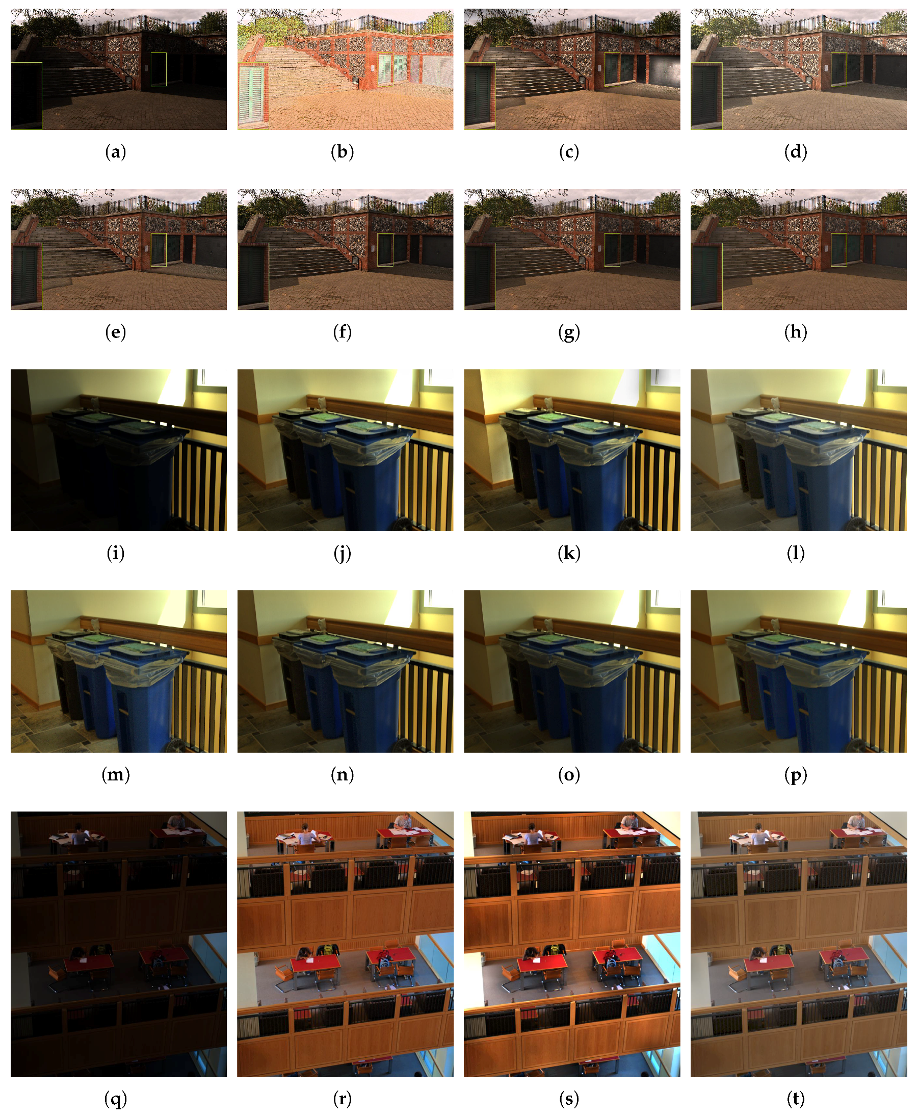
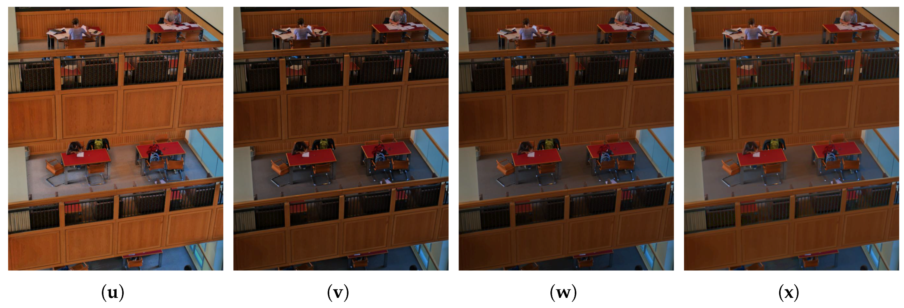
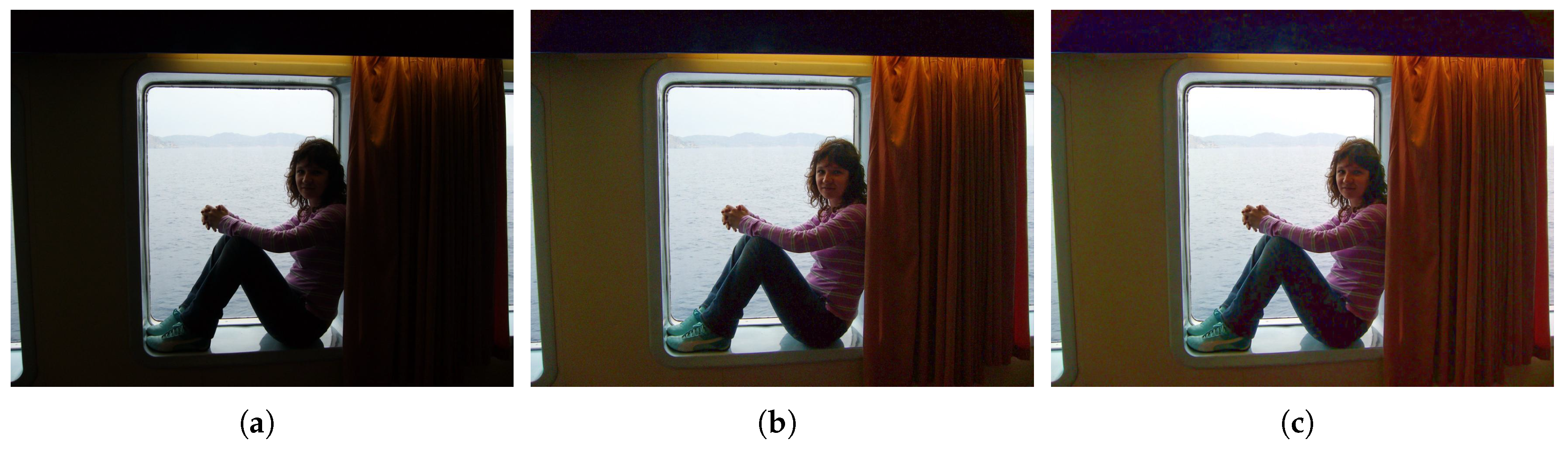
5.2.1. Visual Contrast

In order to have an intuitive impression, the images having complex light are selected from various datasets. As shown in Figure 6, the proposed model can extract more contents from the dark regions.

The proposed model not only performs well for low-light images where the contents are very dark, but also has good performance for images slightly degraded from low light. As shown in Figure 7b, since the fusion process of MF involves histogram equalization, there is the risk of over-exposure. As can be seen from Figure 7c,e,m,s,u, the results of LightenNet and NPE have visible visual artifacts. The result of CRM is not vivid. The results of JIEP are dim; still, there are hidden contents that need to be revealed. FFM(2) only enhances the dark area of FFM(1), the contents of both are the same in the bright areas. Hence, FFM(2) avoids the risk of over-exposure. FFM(2) achieves a good balance in revealing the dark areas and avoids the risk of over-exposure. The proposed model is robust and improves the ability to enhance dark regions.

5.2.2. Lightness Order Error

Lightness order error (LOE) is a method for objectively measuring the naturalness preservation between the original image and its enhanced image, proposed in [12]. The lightness order error can be defined as:

$$LOE=\frac{1}{m}\sum _{x=1}^{m}RD(x),$$

(26)

where m indicates the number of pixels in the image. $RD(x)$ denotes the difference of relative light order between the original image and the enhanced result at the x-th pixel:

$$RD(x)=\sum _{y=1}^{m}U(\mathbf{L}(x),\mathbf{L}(y))\oplus U({\mathbf{L}}^{\prime }(x),{\mathbf{L}}^{\prime }(y)),$$

(27)

$$U(x,y)=\left\{\begin{array}{cc}1,\hfill & \mathrm{when}x\ge y,\hfill \\ 0,\hfill & \mathrm{else}.\hfill \end{array}\right.$$

(28)

⊕ denotes the exclusive-or operator, $\mathbf{L}$ and ${\mathbf{L}}^{\prime }$ are the maximum values among the three color channels (R, G, B) channels of the original image and the enhanced result, respectively. According to [12], the smaller the LOE value, the more natural the enhancement effect. However, LOE doesn’t adequately reflect the enhancement effect. When an algorithm doesn’t have any enhancement to the original image, then the value of LOE is zero.

As shown in

Table 1. Result comparison of Lightness Order Error.

Dataset	NPE [12]	CRM [11]	JIEP [9]	MF [13]	LightenNet [17]	FFM(1)	FFM(2)
Middlebury	359	240	260	207	919	124	224
MF-data	316	402	241	289	807	135	215
NPEpart1	220	575	337	342	720	182	216
NPEpart2	210	504	264	272	747	167	205
NPEpart3	259	568	354	311	785	211	246

, compared to other results, FFM(1) has the lowest LOE due to fractional-order. FFM(2) reveals the dark contents of FFM(1) further, inevitably increasing LOE. While extracting more contents, the LOE of FFM(2) is much lower than the other methods. It can be seen from the given data that the naturalness preservation of the proposed model is efficient.

5.2.3. Images Quality Assessment

A blind image quality assessment called no-reference image sharpness assessment in autoregressive parameter space (ARISM) [35] is used to evaluate the enhanced results. The lower ARISM value represents a higher image quality. There are two ways to calculate ARISM. The one use luminance component (ARISM(1)), and the second use both luminance and chromatic components (ARISM(2)).

As shown in

Table 2. Results of image sharpness quality assessment using ARISM [35].

Dataset	Assessment	NPE [12]	CRM [11]	JIEP [9]	MF [13]	LightenNet [17]	FFM(1)	FFM(2)
Middlebury	ARISM1	3.1909	2.9654	2.8468	2.952	3.0898	2.821	2.7284
	ARISM2	3.4643	3.2278	3.1103	3.2258	3.3712	3.0866	3.0351
MF-data	ARISM1	2.7961	2.7584	2.6982	2.7286	2.7624	2.6858	2.6421
	ARISM2	3.0527	3.0445	2.9511	2.987	3.0127	2.9418	2.9083
NPEpart1	ARISM1	2.7833	2.7521	2.758	2.7356	2.7396	2.7404	2.7064
	ARISM2	3.0252	3.0219	3.0001	2.979	2.9819	2.9801	2.9519
NPEpart2	ARISM1	2.7278	2.6827	2.6877	2.6723	2.6991	2.6688	2.6403
	ARISM2	2.991	2.9676	2.9458	2.9373	2.9573	2.9306	2.9118
NPEpart3	ARISM1	2.9495	2.8561	2.8417	2.8468	2.9352	2.8031	2.7727
	ARISM2	3.1976	3.1346	3.0886	3.0976	3.1785	3.0516	3.0299

, the results of FFM(2) score lowest in image quality assessment. FFM(2) is slightly smaller than FFM(1); this is partly due to the use of filtering operations. FFM(1) get lower scores than the other models. It shows that the use of fractional differential dramatically improves the image quality.

5.2.4. Images Similarity Assessment

The goal of image enhancement is to preserve the other characteristics of the image while enhancing the illumination. To evaluate the similarity between enhanced and original images, A fast reliable image quality predictor (PSIM) [36] and feature similarity (FSIM) [37] are used, which are all based on the human visual system. The PSIM metric combines the gradient magnitude similarities, the color similarity, and reliable perceptual-based pooling [36]. There are two algorithms for FSIM: the one only considers the luminance component i.e., FSIM(1), while another usees both grayscale and color information i.e., FSIM(2).

As shown in

Table 3. Similarity quality assessment metric of input and enhanced images.

Dataset	Assessment	NPE [12]	CRM [11]	JIEP [9]	MF [13]	LightenNet [17]	FFM(1)	FFM(2)
Middlebury	FSIM1	0.7696	0.8117	0.8659	0.8019	0.7427	0.9085	0.8906
	FSIM2	0.7589	0.8054	0.8605	0.7924	0.7325	0.9034	0.8832
	PSIM	0.9954	0.9967	0.9976	0.9960	0.9952	0.9982	0.9976
MF-data	FSIM1	0.8072	0.8127	0.8648	0.8084	0.8179	0.9123	0.8957
	FSIM2	0.8012	0.8078	0.8609	0.8024	0.8122	0.9086	0.8905
	PSIM	0.9964	0.9966	0.9977	0.9966	0.9967	0.9984	0.9979
NPEpart1	FSIM1	0.8911	0.8834	0.9125	0.8869	0.8915	0.9492	0.9457
	FSIM2	0.8883	0.8806	0.9105	0.8839	0.8893	0.9474	0.9433
	PSIM	0.9980	0.9978	0.9985	0.9979	0.9982	0.9989	0.9987
NPEpart2	FSIM1	0.8813	0.8553	0.9096	0.8808	0.8708	0.9421	0.9376
	FSIM2	0.8779	0.8520	0.9073	0.8774	0.8675	0.9398	0.9344
	PSIM	0.9977	0.9973	0.9983	0.9977	0.9976	0.9988	0.9986
NPEpart3	FSIM1	0.8955	0.8752	0.9225	0.8865	0.9038	0.9522	0.9480
	FSIM2	0.8915	0.8710	0.9202	0.8821	0.9006	0.9499	0.9449
	PSIM	0.9976	0.9974	0.9985	0.9976	0.9980	0.9989	0.9987

, the results of FFM(1) have the highest similarity with the original image, and the similarity of FFM(2) is slightly lower than FFM(1), which is much higher than the other methods. The score of FFM(2) is lower than FFM(1) mainly because there is filtering in the fusion framework, which lost a lot of contents. However, the proposed model adds the fusion process based on denoising technique, and the denoise only activates in the low-light areas. Hence, FFM(2) also has a high similarity to the original image. It can be seen from the data that the fractional-order is more powerful in preserving the feature of images, and the distortion of the proposed model is small.

6. Conclusions

In this paper, we introduced a novel fractional-order fusion model for low-light image enhancement, which can extract more contents from dark regions. Firstly, we apply the fractional mask on the input image, and divide the input image into reflectance and illumination. The CRF suitable for the proposed model is used to adjust exposure. Furthermore, the BM3D technique is used to denoise the result, and then another CRF is used to adjust the exposure of the result. Finally, we fuse the original image, the first enhanced image and second enhanced image to get the final enhanced result. The subjective and objective assessments are conducted to check and compare the results. Compared with the state-of-the-art algorithms, the proposed model is efficient in preserving details and extracting contents. The proposed model can be applied in many vision-based applications such as object recognition, image classification, target tracking, facial attractiveness, surveillance, etc.

The limitation of the proposed model is: firstly, as shown in Figure 8, the performance of FFM(1) is good enough. If we use the fusion model to enhance the image (FFM(2)), some dark areas without details will be filled with noise. Although more contents are extracted, the visual effect of the images is degraded. The future work is to find a method to determine whether the areas have contents and whether it needs to be enhanced. Secondly, as shown in

Table 4. Running time comparison of the various methods. These values represent the average time, in seconds.

Dataset	NPE [12]	CRM [11]	JIEP [9]	MF [13]	LightenNet [17]	FFM
Middlebury	20.01	0.67	14.24	0.73	15.91	24.50
MF-data	13.47	0.42	8.58	0.47	10.32	15.70
NPEpart1	10.44	0.37	7.58	0.49	8.09	11.41
NPEpart2	12.66	0.41	11.16	0.45	10.07	14.27
NPEpart3	10.15	0.30	7.01	0.35	7.87	11.82

, the proposed method has no advantage in speed, compared with the other methods. The fractional order requires more information than the integer order, so the processing speed is slow. The proposed method reprocesses the enhanced image again, and it takes more time while extracting more contents. The filtering and fusion operation also increase the running time. In the future, the deep learning strategy could be used to fit the proposed model to run fast.

References

1. Berclaz, J.; Fleuret, F.; Turetken, E.; Fua, P. Multiple object tracking using k-shortest paths optimization. IEEE Trans. Pattern Anal. Mach. Intell. 2011, 33, 1806–1819. [Google Scholar] [CrossRef] [PubMed]
2. Redmon, J.; Divvala, S.; Girshick, R.; Farhadi, A. You only look once: Unified, real-time object detection. Comput. Vis. Pattern Recognit. 2016, 779–788. [Google Scholar]
3. Wang, R.; Wang, G. Medical X-ray image enhancement method based on tv-homomorphic filter. In Proceedings of the International Conference on Image, Vision and Computing, Chengdu, China, 2–4 June 2017; pp. 315–318. [Google Scholar]
4. Cheng, H.D.; Shi, X.J. A simple and effective histogram equalization approach to image enhancement. Digit. Signal Process. 2004, 14, 158–170. [Google Scholar] [CrossRef]
5. Reza, A.M. Realization of the contrast limited adaptive histogram equalization for real-time image enhancement. J. VLSI Signal Process. Syst. Signal Image Video Technol. 2004, 38, 35–44. [Google Scholar] [CrossRef]
6. Dong, X.; Wang, G.; Pang, Y.; Li, W.; Wen, J.; Meng, W.; Lu, Y. Fast efficient algorithm for enhancement of low lighting video. In Proceedings of the IEEE International Conference on Multimedia and Expo, Barcelona, Spain, 11–15 July 2011; pp. 1–6. [Google Scholar]
7. Li, L.; Wang, R.; Wang, W.; Gao, W. A low-light image enhancement method for both denoising and contrast enlarging. In Proceedings of the IEEE International Conference on Image Processing, Quebec City, QC, Canada, 27–30 September 2015; pp. 3730–3734. [Google Scholar]
8. Land, E.H.; Mccann, J.J. Lightness and retinex theory. J. Opt. Soc. Am. 1971, 61, 1–11. [Google Scholar] [CrossRef] [PubMed]
9. Cai, B.; Xu, X.; Guo, K.; Jia, K.; Hu, B.; Tao, D. A joint intrinsic-extrinsic prior model for retinex. In Proceedings of the IEEE International Conference on Computer Vision, Venice, Italy, 22–29 October 2017; pp. 4020–4029. [Google Scholar]
10. Kimmel, R.; Elad, M.; Shaked, D.; Keshet, R.; Sobel, I. A variational framework for retinex. Int. J. Comput. Vis. 2003, 52, 7–23. [Google Scholar] [CrossRef]
11. Ying, Z.; Li, G.; Ren, Y.; Wang, R.; Wang, W. A new low-light image enhancement algorithm using camera response model. In Proceedings of the IEEE International Conference on Computer Vision Workshop, Venice, Italy, 22–29 October 2017; pp. 3015–3022. [Google Scholar]
12. Wang, S.; Zhang, J.; Hu, H.-M.; Li, B. Naturalness preserved enhancement algorithm for non-uniform illumination images. IEEE Trans. Image Process. 2013, 22, 3538–3548. [Google Scholar] [CrossRef] [PubMed]
13. Fu, X.; Zeng, D.; Yue, H.; Liao, Y.; Ding, X.; Paisley, J. A fusion-based enhancing method for weakly illuminated images. Signal Process. 2016, 129, 82–96. [Google Scholar] [CrossRef]
14. Lore, K.G.; Akintayo, A.; Sarkar, S. Llnet: A deep autoencoder approach to natural low-light image enhancement. Pattern Recognit. 2017, 61, 650–662. [Google Scholar] [CrossRef]
15. Gharbi, M.; Chen, J.; Barron, J.T.; Hasinoff, S.W.; Durand, F. Deep bilateral learning for real-time image enhancement. ACM Trans. Graph. 2017, 36, 118. [Google Scholar] [CrossRef]
16. Cai, J.; Gu, S.; Lei, Z. Learning a deep single image contrast enhancer from multi-exposure images. IEEE Trans. Image Process. 2018, 27, 2049–2062. [Google Scholar] [CrossRef] [PubMed]
17. Chongyi, L.; Guo, J.; Porikli, F.; Pang, Y. Lightennet: A convolutional neural network for weakly illuminated image enhancement. Pattern Recognit. Lett. 2018, 104, 15–22. [Google Scholar]
18. Pu, Y.-F.; Zhang, N.; Zhang, Y.; Zhou, J.L. A texture image denoising approach based on fractional developmental mathematics. Pattern Anal. Appl. 2016, 19, 427–445. [Google Scholar] [CrossRef]
19. Pu, Y.-F. Fractional calculus approach to texture of digital image. In Proceedings of the International Conference on Signal Processing, Beijing, China, 16–20 November 2006; pp. 1002–1006. [Google Scholar]
20. Aygören, A. Fractional Derivative and Integral; Gordon and Breach Science Publishers: Philadelphia, PA, USA, 1993. [Google Scholar]
21. Koeller, R.C. Applications of fractional calculus to the theory of Viscoelasticity. Trans. ASME J. Appl. Mech. 1984, 51, 299–307. [Google Scholar] [CrossRef]
22. Rossikhin, Y.A.; Shitikova, M.V. Applications of Fractional Calculus to Dynamic Problems of Linear and Nonlinear Hereditary Mechanics of Solids; McGraw-Hill: New York, NY, USA, 1997. [Google Scholar]
23. Oldham, K.; Spanier, J. The Fractional Calculus Theory and Applications of Differentiation and Integration to Arbitrary Order; Elsevier: Amsterdam, The Netherlands, 1974. [Google Scholar]
24. Lee, S. An efficient content-based image enhancement in the compressed domain using retinex theory. IEEE Trans. Circuits Syst. Video Technol. 2007, 17, 199–213. [Google Scholar] [CrossRef]
25. Pu, Y.-F.; Siarry, P.; Chatterjee, A.; Wang, Z.N.; Zhang, Y.I.; Liu, Y.G.; Zhou, J.L.; Wang, Y. A fractional-order variational framework for retinex: Fractional-order partial differential equation based formulation for multi-scale nonlocal contrast enhancement with texture preserving. IEEE Trans. Image Process. 2018, 27, 1214–1229. [Google Scholar] [CrossRef] [PubMed]
26. Fu, X.; Zeng, D.; Huang, Y.; Zhang, X.P.; Ding, X. A weighted variational model for simultaneous reflectance and illumination estimation. In Proceedings of the Computer Vision and Pattern Recognition, Las Vegas, NV, USA, 27–30 June 2016; pp. 2782–2790. [Google Scholar]
27. Guo, X.; Li, Y.; Ling, H. Lime: Low-light image enhancement via illumination map estimation. IEEE Trans. Image Process. 2017, 26, 982–993. [Google Scholar] [CrossRef] [PubMed]
28. Dabov, K.; Foi, A.; Katkovnik, V.; Egiazarian, K. Image denoising by sparse 3-D transform-domain collaborative filtering. IEEE Trans. Image Process. 2007, 16, 2080–2095. [Google Scholar] [CrossRef] [PubMed]
29. Tseng, P. Convergence of a block coordinate descent method for nondifferentiable minimization. J. Optim. Theory Appl. 2001, 109, 475–494. [Google Scholar] [CrossRef]
30. Candès, E.J.; Wakin, M.B.; Boyd, S.P. Enhancing sparsity by reweighted lsb1 minimization. J. Fourier Anal. Appl. 2007, 14, 877–905. [Google Scholar] [CrossRef]
31. Xu, L.; Yan, Q.; Xia, Y.; Jia, J. Structure extraction from texture via relative total variation. ACM Trans. Graph. 2012, 31, 139. [Google Scholar] [CrossRef]
32. Farbman, Z.; Fattal, R.; Lischinski, D.; Szeliski, R. Edge-preserving decompositions for multi-scale tone and detail manipulation. ACM Trans. Graph. 2008, 27, 1–10. [Google Scholar] [CrossRef]
33. Burt, P.J.; Adelson, E.H. The laplacian pyramid as a compact image Code. Read. Comput. Vis. 1987, 31, 671–679. [Google Scholar]
34. Chakrabarti, A.; Scharstein, D.; Zickler, T.E. An empirical camera model for internet color vision. BMVC 2009, 1, 4. [Google Scholar]
35. Gu, K.; Zhai, G.; Lin, W.; Yang, X.; Zhang, W. No-reference image sharpness assessment in autoregressive parameter space. IEEE Trans. Image Process. Publ. IEEE Signal Process. Soc. 2015, 24, 3218–3231. [Google Scholar]
36. Gu, K.; Li, L.; Lu, H.; Min, X.; Lin, W. A fast reliable image quality predictor by fusing micro- and macro-structures. IEEE Trans. Ind. Electron. 2017, 64, 3903–3912. [Google Scholar] [CrossRef]
37. Zhang, L.; Zhang, L.; Mou, X.; Zhang, D. Fsim: A feature similarity index for image quality assessment. IEEE Trans. Image Process. Publ. IEEE Signal Process. Soc. 2011, 20, 2378. [Google Scholar] [CrossRef]
38. Pu, Y.-F.; Zhou, J.L.; Yuan, X. Fractional differential mask: A fractional differential-based approach for multiscale texture enhancement. IEEE Trans. Image Process. 2010, 19, 491–511. [Google Scholar]
Figure 1. The flow chart of the fusion model.
Symmetry 11 00574 g001
Figure 2. Comparison of different illumination adjustment strategy. (a) the under-exposure image; (b) the Gamma transformation according to Equation (8); (c) the original camera response function (CRF) according to Equation (9); (d) the modified result of CRF; (e) the well-exposure image. (f), (g), (h), (i) and (j) are the three color channels (R, G, B) histograms of (a), (b), (c), (d) and (e), respectively.
Symmetry 11 00574 g002
Figure 3. Multi-scale fusion process weights setting. (a) the original image; (b) the first enhanced image; (c) the second enhanced image; (d) the result of fusion; (e) the weight function.
Symmetry 11 00574 g003
Figure 4. One-dimensional signal processing. (a) the original signal; (b) the signal with Gaussian noise added; (c) the result from Equation (25), v is 2.4 and λ 3 is 1.125 ; (df) the results are from Equation (23), λ 1 is 0.6, 0.8, 1 respectively; (gi) the outputs are from Equation (24), λ 2 is 1.6, 2.4, 3.2, respectively.
Symmetry 11 00574 g004
Figure 5. The impact of fractional-order. (a) the original image; (b) the reflectance from first-order differential is more prominent than fractional-order differential; (c) the reflectance measured with fractional-order differential is more prominent than first-order differential.
Symmetry 11 00574 g005
Figure 6. Comparison of visual contrast in the low-light images which the contents are very dark. (a,i) are original images; (b,j) MF [13]; (c,k) LightenNet [17]; (d,l) CRM [11]; (e,m) NPE [12]; (f,n) JIEP [9]; (g,o) are enhanced images of FFM (1); (h,p) are final results of the proposed model.
Symmetry 11 00574 g006
Figure 7. Comparison of enhancement schemes for images which are slightly degraded from low-light conditions. (a,i,q) are original images; (b,j,r) MF [13]; (c,k,s) LightenNet [17]; (d,l,t) CRM [11]; (e,m,u) NPE [12]; (f,n,v) JIEP [9]; (g,o,w) Our enhanced images of FFM(1); (h,p,x) are final results.
Symmetry 11 00574 g007aSymmetry 11 00574 g007b
Figure 8. An example of a failure case. (a) the original image; (b) the effect of FFM(1); (c) the result of FFM(2).
Symmetry 11 00574 g008