On Efficient Estimation of Process Variability

Abstract

Variability or dispersion plays an important role in any process and provides insight into the spread of data from some central point, usually the mean. A process with less spread is preferred over a process in which values differ greatly from the mean. Various methods are available to estimate the process dispersion by using information on the variable of interest. Certain additional variables provide good insight to estimate the process dispersion. In this paper, we propose an efficient method for the estimation of process variability by using the exponential method. The properties of the proposed method were studied. We conducted simulation and empirical studies to compare the proposed method with some existing methods of estimation of variability. The results of the numerical study show that our proposed method is better than the other methods used in the study.

1. Introduction

The variability or dispersion is an important aspect of a process, as well as of any statistical study. It provides information about spread of data from some central point. In most cases, that central point is the mean of the data; hence, the variance provides insight into the spread. For example, we may be interested to see the spread in the length of some electrical components from a certain pre-assigned target value. It is always required to use methods or to design procedures which produce smaller spread. The dispersion of estimators in any process or in any sample survey is of utmost importance, as the estimators or processes which provide smaller variability are more efficient and, hence, preferred. The dispersion of the process or estimator depends on the variable under study, method of estimation, and information of certain additional variables that can control the dispersion of the process. The information of additional variables can be efficiently utilized to propose the methods which reduce variation of the process or of the estimator. In survey sampling, the estimation of dispersion can be done using different methods which range from simple to complex. Some of these methods utilize the information of additional variables and some do not. The popular methods which utilize the information of additional variables to estimate dispersion are based on the ratio of the study variable to an additional variable and on the linear regression of the study variable to the additional variable. In some cases, the transformation of additional variables plays a useful role in decreasing the variability of the estimators; hence, certain methods are based on the transformed additional variables.

Several authors proposed various methods to estimate the process variation using the information of an additional or auxiliary variable. The method of using the information of an additional variable characterizes a certain estimation method and is very useful in decreasing the variance of estimation.

Several studies were conducted by many researchers to estimate the variability of a process, known as the population variance of the study variable $S_y^2$. The simplest estimator of population variance is the sample variance $s_y^2$, which was proposed by Reference [1]. Some other estimators of variance were proposed in References [2,3,4,5,6,7] and are based on certain information of one or more auxiliary variables (X). The method of using auxiliary information is very useful in proposing efficient estimates of the population variance. Some methods which are useful in the estimation of population variance are given in the following section.

2. Materials and Methods

Suppose we have a finite process which can produce N units; let the value of the characteristic of interest be $U_1,U_2,\dots ,N_N$. Suppose that the variability of the process is to be estimated on the basis of a sample of size n. Let Y represent the variable of interest and X represent the auxiliary variable. Also, let $\overline{Y}$ and $S_y^2$ be the mean and variance of the variable of interest, and let $\overline{X}$ and $S_x^2$ be the mean and variance of the auxiliary variable for the whole process. The corresponding sample measures are $\overline{y},s_y^2,\overline{x}$, and $s_x^2$, respectively. When information on two variables is available, then the strength of interdependence (correlation coefficient) between these variables is of importance and is denoted by ${\rho }_{xy}$. Also, let ${\beta }_2^{/}\left(y\right)$ and ${\beta }_2^{/}\left(x\right)$ be the coefficients of kurtosis of the study and auxiliary variables, and let ${\beta }_1\left(x\right)$ be the squared coefficient of skewness of the auxiliary variable. Some additional notations that are useful in studying the properties of various estimators of population variance are given below.

$$h=\frac{{\mu }_{22}}{{\mu }_{20}{\mu }_{02}};h^{/}=h-1;{\lambda }_{21}=\frac{{\mu }_{21}}{\sqrt{{\mu }_{20}{\mu }_{02}}},where {\mu }_{rs}=\frac{1}{N}{\displaystyle {\sum }_{i=1}^N{\left(Y_i-\overline{Y}\right)}^r{\left(X_i-\overline{X}\right)}^s}$$

.

We also use $s_y^2=S_y^2\left(1+e_0\right)$ and $s_x^2=S_x^2\left(1+e_1\right)$ in practice, such that $E\left(e_0^2\right)={\beta }_2^{/}\left(y\right)$, $E\left(e_1^2\right)=\lambda {\beta }_2^{/}\left(x\right)$, and $E\left(e_0{e}_1\right)=\lambda h^{/}$, with $\lambda =N^{-1}$.

We will now discuss some available estimators for process variability (the population variance).

The usual unbiased estimator of population variance is $t_0=s_y^2$ with the mean-square error (MSE) given as

$$MSE\left(t_o\right)=\frac{1}{n}{S}_y^4\left[{\beta }_2^{/}\left(y\right)-1)\right]$$

(1)

The estimator given above is based on the information of the study variable only. An estimator of variance which utilizes the information of an auxiliary variable was proposed by Reference [1] as

$$t_I=s_y^2\frac{S_x^2}{s_x^2}$$

(2)

The MSE of $t_I$ up to the first order is

$$MSE\left(t_I\right)\approx \frac{1}{n}{S}_y^4\left[{{\beta }^{\prime }}_2\left(y\right)+{{\beta }^{\prime }}_2\left(x\right)-2h^{\prime }\right]$$

(3)

Two exponential-type estimators of variance were proposed by Reference [8] as

$$t_{SR}=s_y^2\exp \left(\frac{S_x^2-s_x^2}{S_x^2+s_x^2}\right)$$

(4)

and

$$t_{SP}=s_y^2\exp \left(\frac{s_x^2-S_x^2}{S_x^2+s_x^2}\right).$$

(5)

The MSE of the estimators in Equations (4) and (5) are, respectively,

$$MSE\left(t_{SR}\right)=\frac{1}{n}{S}_y^4\left[{\beta }_2{}^{\prime }\left(y\right)+\frac{1}{4}{\beta }_2{}^{\prime }\left(x\right)-h^{\prime }\right]$$

(6)

and

$$MSE\left(t_{SR}\right)=\frac{1}{n}{S}_y^4\left[{\beta }_2{}^{\prime }\left(y\right)+\frac{1}{4}{\beta }_2{}^{\prime }\left(x\right)+h^{\prime }\right].$$

(7)

An exponential-type estimator of variance, proposed by Reference [7], is

$$t_A=s_y^2\exp \left(\frac{\overline{X}-\overline{x}}{\overline{X}+\overline{x}}\right)$$

(8)

with MSE as

$$MSE\left(t_A\right)=\frac{1}{n}{S}_y^4\left[{\beta }_2{}^{\prime }\left(y\right)+\frac{1}{4}{C}_x^2-{\lambda }_{21}{C}_x\right],$$

(9)

where $C_x=\overline{X}/S_x$ is the coefficient of variation of the auxiliary variable X. An estimator of variance, based on the coefficient of variations, was proposed by Reference [2] as

$$t_{DT}=s_y^2\left(C_x^2/{\widehat{C}}_x^2\right)$$

(10)

with MSE as

$$MSE\left(t_{DT}\right)=\frac{1}{n}{S}_y{}^4\left[{{\beta }^{\prime }}_2\left(y\right)+\left\{{{\beta }^{\prime }}_2\left(x\right)+4C_x{}^2-4\sqrt{{\beta }_1\left(x\right)}{C}_x\right\}-2\left(h^{\prime }-2{\lambda }_{21}{C}_x\right)\right].$$

(11)

A general procedure for estimating population variance was proposed by Reference [9] as

$$t_{RP}=(s_y^2+d)\left[\omega {\left(C_y^2/{\widehat{C}}_y^2\right)}^{\gamma }+(1-\omega ){\left({\widehat{C}}_y^2/C_y^2\right)}^{\chi }\right]-d$$

(12)

with MSE as

$$MSE\left(t_{RP}\right)=\frac{1}{n}{S}_y{}^4\left[{{\beta }^{\prime }}_2\left(y\right)-\frac{{\left(h^{\prime }-2{\lambda }_{21}{C}_x\right)}^2}{{{\beta }^{\prime }}_2\left(x\right)+4C_x{}^2-4\sqrt{{\beta }_1\left(x\right)}{C}_x}\right].$$

(13)

Various authors have used certain transformations of the auxiliary variable to propose different estimators of variance. The popular transformation used by various authors is $s_x^{2*}=S_x^2\left(1+g\right)-g{s}_x^2$, where $g=n/\left(N-n\right)$; under this transformation, $s_x^{2*}$ is an unbiased estimator for $S_x^2$. Following the same transformation, Reference [6] proposed a dual ratio-type estimator for population variance as

$$t_{YK2}=s_y^2\left(\frac{s_x^{* 2}}{S_x^2}\right)$$

(14)

with MSE given as

$$MSE(t_{YK2})=\frac{1}{n}{S}_y^4\left[{{\beta }^{\prime }}_2\left(y\right)+g^2{{\beta }^{\prime }}_2\left(x\right)-2g{h}^{\prime }\right].$$

(15)

The use of a transformed auxiliary variable provides more efficient estimators of population variance; see, for example, References [6,7,8,9,10,11].

The main purpose of this paper is to propose a generalized exponential estimator for population variance by utilizing transformed auxiliary information. The estimator is proposed in Section 3.

3. Proposed Estimator

Using the concept of Reference [6], we propose two general exponential-type estimators, known as the exponential ratio and exponential product estimators of population variance, by utilizing transformed auxiliary information x. The proposed estimators are as follows:

$$t_{eR}^{}=s_y^2\exp \left(\frac{s_x^{2*}-S_x^2}{S_x^2+s_x^{2*}}\right)$$

(16)

and

$$t_{eP}^{}=s_y^2\exp \left(\frac{S_x^2-s_x^{2*}}{S_x^2+s_x^{2*}}\right),$$

(17)

where $s_x^{2*}=S_x^2\left(1+g\right)-g{s}_x^2$. The MSE of the proposed estimators, up to the first order, are

$$MSE\left(t_{eR}\right)\cong S_y^4 \left[{\beta }_2{}^{\prime }\left(y\right)+\frac{1}{4}{g}^2{\beta }_2{}^{\prime }\left(x\right)-g{h}^{\prime }\right]$$

(18)

and

$$MSE\left(t_{eP}\right)\cong S_y^4\left[{\beta }_2{}^{\prime }\left(y\right)+\frac{1}{4}{g}^2{\beta }_2{}^{\prime }\left(x\right)+g{h}^{\prime }\right].$$

(19)

We have also proposed another estimator, following Reference [11] as

$$t_{eRG}^{}=s_y^2\exp \left[{\beta }_i\left(\frac{s_x^{2*}-S_x^2}{S_x^2+(a_i-1)s_x^{2*}}\right)\right]$$

(20)

or

$$t_{eRG}=s_y^2\exp \left[\beta \left(\frac{g(S_x^2-s_x^2)}{S_x^2+\left(a-1\right)\left\{S_x^2+g(S_x^2-s_x^2)\right\}}\right)\right].$$

(21)

Using $s_y^2=S_y^2\left(1+e_o\right)$ and $s_x^2=S_x^2\left(1+e_1\right)$, and using a Taylor series expansion of Equation (21), we have

$$t_{eRG}^{}-S_y^2\cong S_y^2\left(e_o-\frac{\beta g{e}_1}{a}+\frac{\beta g^2{e}_1{}^2\left(a-1\right)}{a^2}+\frac{{\beta }^2{g}^2{e}_1{}^2}{2a^2}-\frac{\beta g{e}_o{e}_1}{a}\right).$$

(22)

The bias of the proposed estimator, up to the first order, is given as

$$Bias\left(t_{eRG}\right)\cong S_y^2\left(\frac{\beta g^2\left(a-1\right){\beta }_2{}^{\prime }(x)}{a^2}+\frac{{\beta }^2{g}^2{\beta }_2{}^{\prime }(x)}{2a^2}-\frac{\beta g{h}^{\prime }}{a}\right).$$

The MSE of the estimator in Equation (21) is

$$MSE\left(t_{eRG}\right)\cong S_y^4\left({\beta }_2{}^{\prime }(y)+\frac{{\beta }^2{g}^2{\beta }_2{}^{\prime }(x)}{a^2}-2\frac{\beta g{h}^{\prime }}{a}\right).$$

(23)

The optimum value of a_i is obtained by minimizing Equation (23) and is given as

$$a=g.\beta .\frac{{{\beta }^{\prime }}_2(x)}{h^{\prime }}.$$

(24)

Using the optimum value of $a$ in Equation (23), the minimum value of MSE is

$$MS{E}_{\min }(t_{eRG})=\frac{1}{n}{S}_y^4\left[{{\beta }^{\prime }}_2\left(y\right)-\frac{{h^{\prime }}^2}{{{\beta }^{\prime }}_2\left(x\right)}\right].$$

(25)

3.1. Special Cases

The special cases of the proposed estimator are obtained using different values of the constants involved and are given in Table 1.

Table 1. Special cases of the proposed estimator.

Estimator	$\mathit{\beta }$	$\mathit{a}$	g
$t_o=s_y^2$	0	a	g
$t_{eR1}=s_y^2\exp \left(\frac{s_x^{*2}-S_x^2}{S_x^2+\left(a-1\right)s_x^{*2}}\right)$	1	a	g
$t_{eR2}=s_y^2\exp \left(\frac{s_x^{*2}-S_x^2}{S_x^2}\right)$	1	1	g
$t_{eR3}=s_y^2\exp \left(\frac{s_x^{*2}-S_x^2}{S_x^2+s_x^{*2}}\right)=t_{er}$	1	2	g

We now compare the proposed estimator with some popular available estimators of population variance. The efficiency comparison is given in Section 3.2.

3.2. Efficiency Comparison of the Generalized Exponential Estimator

The comparison of the proposed estimator was done by comparing the mean-square error of the proposed estimator with that of some available estimators. We compared our proposed estimator with $t_o$, $t_I$, $t_{SR}$, and $t_{YK2}$ given in Section 2. The mean-square errors of these estimators are given in Equations (1), (3), (6), and (15), respectively.

Now, the comparison of the proposed estimator with $t_0$ shows that

$$MSE\left(t_{eRG}\right)-MSE\left(t_o\right)<0 if a>g{{\beta }^{\prime }}_2\left(x\right)/2h^{/}.$$

The comparison of $t_{eRG}$ with $t_I$ shows that

$$MSE\left(t_{eRG}\right)-MSE\left(t_I\right)<0 if g<a<g{{\beta }^{\prime }}_2\left(x\right)/\left[2h^{\prime }-{{\beta }^{\prime }}_2\left(x\right)\right].$$

Again, the comparison of $t_{eRG}$ with $t_{SR}$ shows that

$$MSE\left(t_{eRG}\right)- MSE\left(t_{SR}\right)<0 if \frac{2g{{\beta }^{\prime }}_2\left(x\right)}{4h^{\prime }-{{\beta }^{\prime }}_2\left(x\right)}<a<2g.$$

The comparison of $t_{eRG}$ with $t_{YK2}$ shows that

$$MSE\left(t_{eRG}\right)- MSE\left(t_{YK2}\right)<0 if \frac{g{{\beta }^{\prime }}_2\left(x\right)}{2h^{\prime }-g{{\beta }^{\prime }}_2\left(x\right)}<a<1.$$

We now give numerical examples for the application of the proposed estimator.

4. Results

In this section, we present the numerical studies for the application of the proposed generalized estimator of population variance. The numerical study is twofold. We firstly provide 10 real examples by considering 10 real populations; later, we provide a simulation study to see the performance of the proposed generalized estimator of variance. The results of these studies are given in the sections below.

4.1. Numerical Study

In this section, we present a numerical study to see the performance of the proposed estimator in estimating the variability of processes. These studies were conducted using 10 real populations which were previously used by various authors to see the performance of their proposed estimators. The description of these populations can be found in the source given.

The summary measures for these 10 populations are given in Table 2. The summary measures of two populations indicate that the study variable and auxiliary variable are highly correlated. This is generally an underlying requirement for ratio- and exponential-type estimators for the estimation of population characteristics.

Table 2. Summary measures for populations.

Measure	Source	N	n	$\overline{\mathit{Y}}$	$\overline{\mathit{X}}$	${\mathit{C}}_{\mathit{y}}$	${\mathit{C}}_{\mathit{x}}$
Population I	[12]	142	20	4015.218	2900.387	2.112	2.197
Population II	[13]	80	25	5182.638	283.875	0.352	0.943
Population III	[14]	64	8	141.500	51.187	0.537	0.509
Population IV	[15]	51	7	13.067	543.373	0.323	0.684
Population V	[16]	58	12	85.948	93.000	1.121	1.127
Population VI	[16]	80	23	90.813	104.575	0.392	0.379
Population VII	[17]	53	10	917.019	1417.245	0.402	0.682
Population VIII	[17]	66	14	974.424	1716.136	0.512	0.612
Population IX	[18]	71	12	4137.803	241.944	0.306	0.557
Population X	[18]	75	12	1.377	6.347	1.748	0.418
Measure	Source	${\mathit{\rho }}_{\mathit{x}\mathit{y}}$	${\mathit{\beta }}_{\mathbf{2}}\left(\mathit{y}\right)$	${\mathit{\beta }}_{\mathbf{2}}\left(\mathit{x}\right)$	${\mathit{\beta }}_{\mathbf{1}}\left(\mathit{x}\right)$	$\mathit{h}$	${\mathit{\lambda }}_{\mathbf{21}}$
Population I	[12]	0.995	40.854	48.157	40.218	43.762	5.979
Population II	[13]	0.914	2.267	3.650	1.295	2.337	0.548
Population III	[14]	−0.818	2.378	1.658	0.006	1.438	−0.146
Population IV	[15]	0.446	3.653	15.231	7.636	4.472	0.942
Population V	[16]	0.978	24.747	6.175	3.333	5.167	155.121
Population VI	[16]	0.628	4.573	5.701	0.629	10.772	96.058
Population VII	[17]	0.775	5.355	8.526	5.668	4.839	562.914
Population VIII	[17]	0.776	9.128	19.038	11.960	11.210	1142.321
Population IX	[18]	−0.382	4.458	2.635	0.255	2.181	247.516
Population X	[18]	0.222	31.544	2.019	0.004	4.271	4.027

We computed the mean-square error of various estimators using the data of above populations. After computing the mean-square error, we computed the percent relative efficiency (PRE) of various estimators, relative to $t_0$, using Equation (26).

$$PRE=\frac{MSE\left(t_i\right)}{MSE\left(t_0\right)}\times 100;i=I,SR,A,YK2,rP,eR,eRG.$$

(26)

The efficiency provides information about the sample size required to achieve a desired result, using an estimator that is provided by the base estimator $t_0$ with a sample of size 100. This, therefore, means that a smaller value of PRE indicates that the estimator is more efficient. The results are given in Table 3.

Table 3. Percent relative efficiency (PRE) of various estimators.

Population Number	Estimator
	${\mathit{t}}_0$	${\mathit{t}}_{\mathit{I}}$	${\mathit{t}}_{\mathit{S}\mathit{R}}$	${\mathit{t}}_{\mathit{A}}$	${\mathit{t}}_{\mathit{Y}\mathit{K}2}$	${\mathit{t}}_{\mathit{r}\mathit{P}}$	${\mathit{t}}_{\mathit{e}\mathit{R}}$	${\mathit{t}}_{\mathit{e}\mathit{R}\mathit{G}}$
1	100	33.731	22.284	135.988	81.601	36.427	83.205	21.703
2	100	98.106	46.764	158.333	56.739	96.203	56.552	41.038
3	100	84.202	80.172	99.312	110.281	95.337	82.673	68.061
4	100	174.642	103.215	128.675	86.316	78.946	73.917	59.606
5	100	31.169	81.740	77.460	81.330	82.980	74.525	10.052
6	100	37.034	63.532	85.541	83.752	57.028	77.202	11.427
7	100	96.512	55.054	89.234	82.016	86.182	72.476	48.790
8	100	70.693	29.870	87.055	58.140	84.745	64.014	25.314
9	100	78.955	77.656	74.898	72.663	75.669	82.562	65.989
10	100	81.918	90.125	105.364	92.336	100.016	84.913	54.820

We can see, from Table 3, that the proposed estimator $t_{eRG}$ is the most efficient estimator, as this estimator requires the least number of observations to obtain a desired result as obtained by $t_0$ with a sample of size 100. We then conducted a regression analysis to see the effect of the correlation coefficient and coefficient of skewness of the auxiliary variable on the efficiency of the estimator. The regression model that we built is as follows:

$$PRE={\widehat{\beta }}_0+{\widehat{\beta }}_1{\rho }_{xy}+{\widehat{\beta }}_2\left\{{\beta }_2\left(x\right)\right\}.$$

The regression summary alongside the result of the test of significance for each estimator is given in Table 4.

Table 4. Regression summary for various estimators.

Coefficient	Estimator
	${\mathit{t}}_{\mathit{I}}$	${\mathit{t}}_{\mathit{S}\mathit{R}}$	${\mathit{t}}_{\mathit{A}}$	${\mathit{t}}_{\mathit{Y}\mathit{K}2}$	${\mathit{t}}_{\mathit{r}\mathit{P}}$	${\mathit{t}}_{\mathit{e}\mathit{R}}$	${\mathit{t}}_{\mathit{e}\mathit{R}\mathit{G}}$
${\widehat{\beta }}_0$	88.449 (0.003)	82.312 (0.000)	94.493 (0.000)	86.106 (0.000)	90.983 (0.000)	76.948 (0.000)	53.468 (0.000)
${\widehat{\beta }}_1$	−11.353 (0.700)	−9.407 (0.474)	7.131 (0.701)	−16.670 (0.097)	0.795 (0.930)	−10.860 (0.058)	−26.908 (0.030)
${\widehat{\beta }}_2$	−0.408 (0.748)	−0.798 (0.181)	0.573 (0.482)	0.175 (0.656)	−1.063 (0.026)	0.282 (0.217)	−0.052 (0.907)
F-ratio	0.251 (0.785)	2.420 (0.159)	0.624 (0.482)	1.946 (0.213)	4.898 (0.047)	2.618 (0.142)	4.849 (0.048)

From the above table, we can see that the average efficiency of our proposed estimator, $t_{eRG}$, is the lowest, as ${\widehat{\beta }}_0$ for this estimator has the smallest value. We can also see that the correlation coefficient has a significant effect on the efficiency of $t_{eRG}$, and the regression model for this estimator is significant at 5%. The value of ${\widehat{\beta }}_0$ for our proposed estimator $t_{eR}$ is the second lowest, which indicates that this estimator is the second best estimator for the estimation of population variance. The regression coefficient ${\widehat{\beta }}_2$ is significant at 10% for this estimator, which indicates that the correlation coefficient between the study and auxiliary variables will provide useful information to predict the efficiency of estimator $t_{eR}$. The other significant regression model is for $t_{rP}$; for this estimator, the coefficient of ${\widehat{\beta }}_2$ is significant. This indicates that the coefficient of kurtosis of the auxiliary variable has a significant effect on the efficiency of this estimator. We can also see from Table 4 that the estimator $t_A$ showed the worst performance in this study, as coefficient ${\widehat{\beta }}_0$ for this estimator has the highest value.

We also show the efficiencies of various estimators in Figure 1, where estimators are numbered from 1 to 7 in the order in which they appear in Table 4. This means that estimator $t_I$ is numbered 1 and estimator $t_{eRG}$ is numbered 7. The graph also shows that our proposed estimator $t_{eRG}$ is the most efficient estimator in this study.

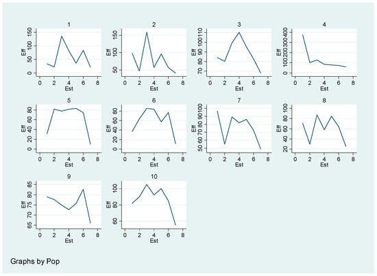
Figure 1. Population wise efficiency comparison.

We now present the results of the simulation study in Section 4.2.

4.2. Simulation Results

In this section, we give the results of the simulation study to see the performance of our proposed estimator. The simulation study was conducted by generating populations of size 500 having a specific correlation structure between the study and auxiliary variables. For each of the populations with a specific correlation coefficient, various estimators were computed. The process was repeated 20,000 times, and we then computed the mean0square error of each estimator alongside the percent relative efficiency as defined in Equation (26). The results of this simulation study are given in Table 5.

Table 5. Percentage relative efficiency (PRE) of existing estimators.

$\mathit{\rho }$	Estimator
	${\mathit{t}}_0$	${\mathit{t}}_{\mathit{I}}$	${\mathit{t}}_{\mathit{S}\mathit{R}}$	${\mathit{t}}_{\mathit{A}}$	${\mathit{t}}_{\mathit{Y}\mathit{K}2}$	${\mathit{t}}_{\mathit{r}\mathit{P}}$	${\mathit{t}}_{\mathit{e}\mathit{R}}$	${\mathit{t}}_{\mathit{e}\mathit{R}\mathit{G}}$
−0.9	100	189.134	119.577	100.037	100.031	109.366	91.881	84.899
−0.7	100	193.632	121.793	100.038	100.518	109.607	88.730	82.266
−0.5	100	196.582	123.296	100.042	100.857	109.711	87.862	86.497
−0.3	100	198.862	124.449	100.047	101.115	109.763	91.445	85.654
−0.1	100	199.721	124.892	100.040	101.216	109.776	92.079	87.677
0.1	100	200.035	124.974	100.038	101.221	109.772	87.667	84.565
0.3	100	198.773	124.377	100.040	101.094	109.762	90.272	88.006
0.5	100	196.642	123.334	100.043	100.866	109.715	88.728	83.709
0.7	100	192.997	121.545	100.045	100.475	109.584	92.261	82.935
0.9	100	189.171	119.600	100.043	100.037	109.366	89.811	86.255

The results of the simulation study clearly indicate that our proposed estimator outperformed other estimators used in the study; hence, we can say that our proposed estimator will estimate process variability with the least error. The efficiency of various estimators is given in Figure 2 below

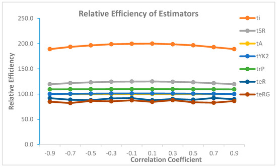
Figure 2. Efficiency comparison with respect to correlation coefficient.

From above figure we can see that our proposed estimator is most efficient for all values of correlation coefficient.

5. Conclusions and Recommendations

In this paper, we proposed a new method for the estimation of process dispersion when the information on a variable of interest and an auxiliary variable is available. We see that the proposed estimator can provide certain other estimators as a special case. We obtained the mean-square error of the proposed estimator and found that the mean-square error of our proposed estimator was less than the mean-square error of other available estimators of variability. We conducted numerical and simulation studies to see the performance of our proposed estimator, and we found that our proposed estimator estimates process variability with the least error. We can, therefore, conclude that our proposed estimator can be used for the estimation of process variability in various areas, including quality control and engineering.

References

- Isaki, C.T. Variance Estimation Using Auxiliary Information. J. Am. Stat. Assoc. 1983, 78, 117–123. [Google Scholar] [CrossRef]
- Das, A.K.; Tripathi, T. Use of Auxiliary Information in Estimating the Finite Population Variance. Sankhya 1978, 40, 139–148. [Google Scholar]
- Upadhyaya, L.; Singh, H. An Estimator for Population Variance That Utilizes the Kurtosis of an Auxiliary Variable in Sample Surveys. Vikram Math. J. 1999, 19, 14–17. [Google Scholar]
- Kadilar, C.; Cingi, H. Ratio Estimators for the Population Variance in Simple and Stratified Random Sampling. Appl. Math. Comput. 2006, 173, 1047–1059. [Google Scholar] [CrossRef]
- Upadhyaya, L.N.; Singh, H.P.; Chatterjee, S.; Yadav, R. A Generalized Family of Transformed Ratio-Product Estimators in Sample Surveys. Model Assist. Stati. Appl. 2011, 6, 137–150. [Google Scholar] [CrossRef]
- Yadav, S.K.; Kadilar, C. A Class of Ratio-Cum-Dual to Ratio Estimator of Population Variance. J. Reliab. Stat. Stud. 2013, 6, 29–34. [Google Scholar]
- Asghar, A.; Sanaullah, A.; Hanif, M. Generalized Exponential Type Estimator for Population Variance in Survey Sampling. Revista Colombiana de Estadística 2014, 37, 213–224. [Google Scholar] [CrossRef]
- Singh, R.; Chauhan, P.; Sawan, N.; Smarandache, F. Improved Exponential Estimator for Population Variance Using Two Auxiliary Variables. arXiv Preprint, 2009; arXiv:0902.0126. [Google Scholar]
- Yadav, R.; Upadhyaya, L.N.; Singh, H.P.; Chatterjee, S. A Generalized Family of Transformed Ratio-Product Estimators for Variance in Sample Surveys. Commun. Stat.-Theory Methods 2013, 42, 1839–1850. [Google Scholar] [CrossRef]
- Sharma, B.; Tailor, R. A New Ratio-Cum-Dual to Ratio Estimator of Finite Population Mean in Simple Random Sampling. Glob. J. Sci. Front. Res. 2010, 10, 27–31. [Google Scholar]
- Sanaullah, A.; Ali, H.A.; ul Amin, M.N.; Hanif, M. Generalized Exponential Chain Ratio Estimators under Stratified Two-Phase Random Sampling. Appl. Math. Comput. 2014, 226, 541–547. [Google Scholar] [CrossRef]
- Das, A.K. Contributions to the Theory of Sampling Strategies Based on Auxiliary Information. Unpublished. Ph.D. Thesis, B.C.K.V., West Bengal, India, 1980. [Google Scholar]
- Murthy, M. Sampling Theory and Methods; Calcutta Statistical Publishing Society: Kolkatta, India, 1967. [Google Scholar]
- Available online: https://www.statcrunch.com/app/index.php?dataid=285946 (accessed on 26 January 2019).
- Gujarati, D.N.; Porter, D.C. Basic Econometrics, 5th ed.; McGraw Hill: New York, NY, USA, 2011; p. 189. [Google Scholar]
- Cochran, W.G. Sampling Technique; John Wiley: New York, NY, USA, 1977. [Google Scholar]
- Singh, R.K.; Chaudhary, B.D. Biometrical Method in Quantitative Genetics Analysis; Kalyani Publishers: New Delhi, India, 1987. [Google Scholar]
- Mukhopadhyay, P. Theory and Methods of Survey Sampling; Prentice Hall: New Delhi, India, 1998. [Google Scholar]
© 2019 by the authors. Licensee MDPI, Basel, Switzerland. This article is an open access article distributed under the terms and conditions of the Creative Commons Attribution (CC BY) license (http://creativecommons.org/licenses/by/4.0/).