Abstract
The current network information asymmetry is infringing the interests of end users in non-neutral network environment. To empower users, application-level performance measurements are usually used to rebalance the information asymmetry currently disfavoring users. Application-level packet loss rate, as an important key performance indicator (KPI), receives extensive attention in academia. However, every coin has its two sides. Although the application-level packet loss estimation is simple and nonintrusive, since the information available from the application layer is relatively scarce compared to the lower layers, the estimation accuracy has no guarantee. In view of this, taking the L-Rex model as the cut-in spot, this paper focuses on leveraging the self-clocking mechanism of Transmission Control Protocol (TCP) to improve the accuracy of application-level loss estimation. Meanwhile, owing to the dynamically estimated parameters and the weakened packet reordering impact, the robustness of estimation is also expected to be improved accordingly. Finally, a series of comparative experiments at the practically relevant parameter space show that the enhanced approach and strategy detailed in this paper are effective.
1. Introduction
The internet was originally designed to be neutral and primarily provide service for time-insensitive traffic. However, with the development of the network, users put forward higher requirements for network services than just being able to obtain information from the internet. Moreover, due to the increasing amount of data, the diversity of applications (e.g., the rise of time-sensitive applications), and the competitive nature of the internet service providers (ISP) industry, although Internet Protocol (IP) packets are still best-effort forwarding without guaranteeing delivery, the intermediate nodes usually process data by priority aimed at achieving differentiated quality of service (QoS) [1,2,3], which makes the network no longer neutral [4].
It is no doubt that some stakeholders will benefit from such non-neutrality, such as high-priority users who pay more fees [5]. Of course, some scholars [6] also believed that, if non-neutrality is well implemented, it will benefit all. However, now, the diversity and heterogeneity of applications and services, as well as the complex infrastructure in behind, present new challenges and make it difficult to implement effective non-neutrality that satisfies everyone. In general, the non-neutrality prioritizes privileged traffic, i.e., the high-priority traffic has a specific performance lower bound, while the low-priority traffic has a performance upper bound but no performance lower bound. Moreover, the current network is information asymmetric, and end users know much less than network operators, internet service providers (ISP), and content providers [7]. Such information asymmetry, especially in a non-neutral network environment, will seriously infringe the interests of end users. This damage is ultimately reflected on the deterioration of the user’s quality of experience (QoE), and, for some ordinary users, the extent of such bad QoE naturally has no lower bound due to the lack of performance lower bound guarantees. Therefore, the quantitative characterization and accurate evaluation of an end user’s QoE are the premise of guaranteeing the interests of end users (when end users realize their interests are infringed, they can fully exercise their market rights by reasonably switching ISPs). Again, since QoE is subjective and abstract, the effective characterization and evaluation of QoE is based on the accurate measurement of QoS. Accordingly, light and user-friendly application-level QoS measurement is conducive to promoting large-scale user installation and, thus, quickly reversing the information asymmetry [8]. Among the numerous key performance indicators (KPI) indicating QoS, application-level packet loss rate, as an important KPI, is widely studied and measured [9,10,11,12]. However, as said by Basso et al., “the collected data in the application layer is more coarse-grained than the data collected with kernel-level measurements” [8]. Therefore, the available traffic information related to packet losses is less in application-level packet loss estimation, which poses a challenge to the estimation accuracy. In view of this, taking the L-Rex model [8] as the cut-in spot, this paper focuses on improving the accuracy and robustness of application-level loss estimation. That is, leveraging the TCP’s self-clocking mechanism [13], we mine the information contained in the burst-gap traffic patterns to dynamically estimate the two decisive parameters required by L-Rex. To rebalance the robustness, the effect of packet reordering is also considered. Also, a series of comparative experiments performed with real measured data and testbed measurements eventually show that the improved L-Rex (IM-L-Rex) is effective for the entire measured parameter space. In this paper, we firstly recall the application-level loss rate estimation model L-Rex and specify its limitations. Then, we utilize the TCP’s self-clocking mechanism to dynamically estimate the two decisive parameters required by L-Rex and exclude the effect of packet reordering. After that, to elaborate the model, we describe the implementation of IM-L-Rex. Finally, we detail and discuss the comparative experiments performed with real measured data and testbed measurements.
The remainder of this paper is organized as follows. Section 2 outlines the L-Rex model and its limitations. Section 3 sketches our enhanced version with an eye toward overcoming the deficiencies of L-Rex model. Section 4 details the implementation of IM-L-Rex. Section 5 presents the comparative experiment results. Section 6 concludes the paper.
2. L-Rex Model
The difficulty in application-level packet loss estimation is how to use the information available only from the application layer to achieve loss estimation and be as accurate as possible. It is well known that, for TCP, the packet loss detection and repair are controlled by the transport layer, while what the application layer has and can contact with the lower transport layer are just a series of system calls. In this case, the L-Rex is naturally based on the system calls to estimate the application-level packet loss rate. Specially, it is inspired by the empirical observation about the dynamics of data returned by the recv() system call. Under the current TCP/IP architecture, packet loss is repaired with retransmission. Accordingly, it is almost a natural idea to take retransmissions as building blocks to construct loss estimation algorithms [14,15,16,17,18,19]. Likewise, L-Rex is also built on the retransmission patterns. The difference lies in that L-Rex mines the hidden retransmission events contained in the data sequence returned by the application-layer recv(). As a result, there is little information available and the problem becomes more challenging.
2.1. Model Description
In the absence of packet loss, the data sequence returned by recv() has the following features:
- (a)
- The recv() will be triggered and return a typical number of bytes as soon as data are available;
- (b)
- During a burst, the time interval between two consecutive recv() is very small;
- (c)
- The “silence period” between two consecutive bursts is usually smaller than Round Trip Time (RTT).
In the case of packet loss, the data sequence returned by recv() appears as follows:
- (A)
- The recv() is blocked due to packet loss, which makes the silence period longer; in the best case (i.e., fast retransmission), an additional RTT is needed to re-trigger recv();
- (B)
- When the lost packet(s) are repaired, a large and non-typical number of bytes will be returned to userspace.
On the basis of the above observations, Basso et al. [8] found that many losses followed the pattern indicated by (A) and (B), i.e., a longer silence period, and a large, non-typical returned number of bytes. Therefore, L-Rex scans the data sequence returned by recv() and counts the number of following cases to achieve the estimation for packet losses:
- (i)
- The time elapsed since the previous recv() is greater than H · RTT;
- (ii)
- The number of received bytes is greater than 1 MSS and less frequent than K;
where H is the smoothing parameter, and K is the ratio of the maximum number of bytes returned by recv() at a time to the total number of bytes received by the receiver during a TCP transfer.
Once the number of estimated packet losses is determined, the estimated application-level packet loss rate (APLREST) is calculated as
where Losses is the number of estimated packet losses, Received_bytes is the total number of bytes received by the receiver during a TCP transfer, and MSS is the maximum segment size obtained through getsockopt().
2.2. Limitations of L-Rex
As a key parameter, the accurate estimation of RTT is crucial to L-Rex. However, in L-Rex implementation, the RTT value is the connect delay, i.e., the time required for the connect() system call to complete. In general, the RTT at the TCP connection establishment is not completely consistent with that after the transmission is stable. For a TCP flow, after the transmission is stable, with the increase of the sending window and the limitation of the bottleneck bandwidth, the RTT may increase due to the queuing problem at the bottleneck. Although Basso et al. used the parameter H to smooth RTT (H · RTT), the value of H is set to 0.7, which is still statically assigned. Similarly, the parameter K is also static in L-Rex implementation with a value of 1%. As we know, due to the packet dynamics along the network path and the diversity of the network that the packets travel through, it is impossible for static parameters to be applicable to all loss patterns. Therefore, the robustness of L-Rex is poor, and the accuracy in practical applications is also difficult to guarantee.
In addition, relying solely on the information available from the data receiver side cannot achieve completely accurate RTT estimation, together with the fact that packet reordering [20] can also result in the pattern indicated by (A) and (B), which will eventually fool L-Rex’s detection rules (i) and (ii). For instance, in Figure 1, the sender sends four data packets; the first two are successfully received and returned to the user space, but due to the delayed D3 caused by packet reordering, the time difference between the last two packets and the first two packets is greater than or equal to the estimated RTT. This situation is in line with the detection rules (i) and (ii), which fools L-Rex. Therefore, distinguishing the pattern caused by packet reordering from that indicated by (A) and (B) is also beneficial to further improve the estimation accuracy of L-Rex.
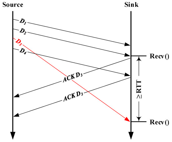
Figure 1.
Sample of packet reordering.
3. IM-L-Rex
3.1. Self-Clocking Mechanism
In the network, the number of active flows carried by a single router is huge, while, in core routers, it can even reach thousands or even more. All of these flows have no any specific information about the network state, which is especially true for TCP/IP networks. At the same time, TCP is greedy, but it does not know which transmission rate to use to ensure high resource utilization without overloading the network. In this case, it can only slowly increase the size of the congestion window through a strategy known as slow start until congestion happens; then, it will reduce the sending rate and the congestion window in respond to the congestion. In this way, it will loop back and forth until the data transfer is completed. Such a reciprocating process is called TCP’s self-clocking mechanism and eventually produces a traffic pattern where the packets are sent in bursts and the spacing between the bursts is probably preserved from one round trip to the next. Although the bursts (e.g., split or merged) and spacing may be changed due to the packet losses or competing traffic, the changes happen infrequently, and the bursts are preserved for at least several round trips after each change.
3.2. Methodology
By detecting the repeated burst-gap patterns, TCP’s self-clocking mechanism is widely used to dynamically estimate RTT and follow changes in the RTT throughout the lifetime of a TCP session [13,21,22]. Since recv() will be triggered as soon as data are available, the self-clocking (or burst-gap) patterns are also passed to the application layer. This provides us with the possibility to dynamically estimate RTT required by L-Rex utilizing the self-clocking mechanism. Autocorrelation is the correlation (similarity) of a dataset with a delayed copy of itself, as a function of the time lag between the datasets. The discrete autocorrelation analysis is a mathematical tool for finding repeating patterns, such as the periodic burst-gap pattern obscured by noise in TCP’s self-clocking mechanism. Similar to Veal et al.’s work [21], in this paper, combined with the TCP self-clocking mechanism, we leverage discrete autocorrelation analysis to realize RTT dynamic estimation. Specifically, the estimation is repeated once per measurement interval T. During this interval, array P(t) ranging from 1 to T is used to store the number of segments that arrive with timestamp t. Once an interval time T is expired, the discrete autocorrelation is calculated for each lag from 1 to l/2, and the estimated RTT is the max(R), where is calculated as
where the measurement interval time T is supplied as a parameter and determines the upper bound on the maximum RTT that can be measured; in our implementation, T is set to 500 ms. Also, to overcome the multiple burst-gap patterns, the limit of fractional lags and the maximum correlation percentage are set to 1/4 and 75%, respectively, while the lower bound RTT is set to min (10 ms, the Nyquist period within T) to exclude the effect of extremely small lags caused by the noises like competing traffic, back-to-back received packets, and other network conditions disrupting the burst-gap patterns.
Since RTT is dynamically estimated, the parameter H used for smoothing RTT is no longer needed in our loss detection. Moreover, regarding parameter K, the number of received segments at a time, no matter how non-typical, will not exceed the number of segments sent by the sender in one sending round. In this case, we use the peak value of the strong correlation corresponding to the estimated RTT to infinitely approximate the maximum number of segments sent within T, i.e., the parameter K is dynamically computed as
where Bytes_peak is the maximum number of segments sent in all sending rounds within one measurement interval T.
In order to cope with the problem of packet reordering, we explore distinguishing the pattern caused by packet reordering from that indicated by (d) and (e). In fact, just like L-Rex’s full name “Likely Rexmit”, L-Rex estimates packet losses by identifying likely “rexmit” (i.e., retransmissions). For a loss event during a TCP transfer, we noted that the retransmission(s) used for repairing it are either triggered by a fast retransmission or triggered by an overtime retransmission. Therefore, a loss event is either repaired with a group of retransmission(s) that begin with fast retransmission or repaired with a group of retransmission(s) that begin with overtime retransmission. In view of this, we introduce the following definitions:
Definition 1 (Fast loss event):
It is repaired with a group of retransmission(s) that begin with fast retransmission.
Definition 2 (Overtime loss event):
It is repaired with a group of retransmission(s) that begin with overtime retransmission.
By Definition 1 and Definition 2, the retransmissions used for repairing the loss events during a TCP transfer can be divided into the following two categories:
As shown in Figure 2, to exclude the effect of packet reordering, instead of adopting the L-Rex’s traditional way of identifying retransmissions coarsely, we further refine the loss set determined by (i) and (ii) to screen out the retransmissions belonging to set F∪O. If N and M denote the number of fast loss events and the number of overtime loss events in a TCP connection, respectively, then the number of retransmissions belonging to set F∪O (i.e., the retransmissions used for repairing the loss events in a TCP connection) can be calculated as
where Fasti denotes the number of retransmissions used for repairing the ith fast loss event, and Overtimej denotes the number of retransmissions used for repairing the jth overtime loss event.
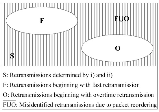
Figure 2.
Retransmissions determined by (i) and (ii).
Referring to Equation (4), to determine Retransrepair, we firstly need to identify each loss event in a TCP connection and then determine the retransmissions used for repairing it.
For fast loss event, we identify it by detecting the first fast retransmission used for repairing it. Without loss of generality, a fast retransmission is caused by more than or equal to four out-of-order arrivals that appear at the receiver side in the following two forms:
- Form 1: The out-of-order arrivals are continuous and can be returned by recv() at one time. For instance, in Figure 3a, the four continuous out-of-order arrivals result in recv() returning to userspace at least five segments at a time (i.e., the fast retransmission used for repairing the lost packet plus the four continuous out-of-order segments that arrived while recv() was blocked).
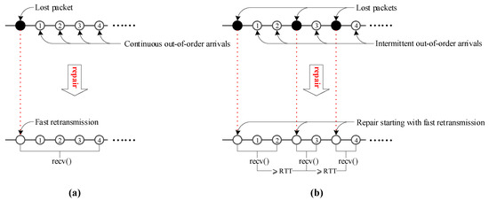 Figure 3. Fast loss event scenario. (a) Continuous out-of-order arrivals; (b) Intermittent out-of-order arrivals.
 - Form 2: The out-of-order arrivals are intermittent (discontinuous) and need at least two recv()s to be returned to userspace; the first recv() is triggered by a fast retransmission, while the time interval between the subsequent recv() and the previous recv() is greater than RTT. For instance, in Figure 3b, the four out-of-order arrivals triggering fast retransmission require calling recv() three times to return to user space. In this case, the recv () triggered by the first fast retransmission returns a fast retransmission and the first two out-of-order arrivals; after RTT, the recv() triggered by the second retransmission returns a retransmission and the third out-of-order arrival; after another RTT, recv() triggered by the third retransmission returns a retransmission and the fourth out-of-order arrival.
Based on the discussion above, assume that the data sequence returned by recv() during a TCP transfer is described with set S = {<R1, T1, B1>, …, <Rn, Tn, Bn>}, where ∀i ∊ N, <Ri, Ti, Bi> denotes the ith group data returned by recv(), Ri denotes the byte length of <Ri, Ti, Bi>, Ti denotes the timestamp of <Ri, Ti, Bi>, Ti ≤ Ti+1, and Bi is a Boolean variable. Then, <Ri, Ti, Bi> is the first fast retransmission used for repairing a fast loss event if and only if Bi = 1, where Bi reports the following:
where Li indicates the last recv() corresponding to the identified fast loss event and can be calculated as
From Figure 3, we can see that, for an identified fast lost event, the number of retransmissions used for repairing it depends on the number of recv()s corresponding to it. Therefore, after identifying the fast loss event, Fasti can be calculated as
For an overtime loss event, we identify it by detecting the first overtime retransmission used for repairing it. Since the overtime retransmission is caused by an expired retransmission timeout (RTO) timer, <Rj, Tj, Bj> is the first overtime retransmission used for repairing an overtime loss event if and only if Bj = 1, where Bj reports the following:
Referring to RFC6298 [23], once RTT is dynamically measured, RTO can be calculated as
where RTTS is the smoothed RTT and RTTD is the weighted average of the deviation of RTT. They can be calculated as follows:
where α is an empirical constant, and the value of this constant is 1/8.
where β is an empirical constant, and the value of this constant is 1/4.
Likewise, as shown in Figure 4, for an overtime loss event, the number of retransmissions used for repairing it also depends on a group of recv()s with a time interval greater than RTT. Therefore, Overtimej can be calculated as
where Lj indicates the last recv() corresponding to the identified overtime loss event, and it can be calculated as
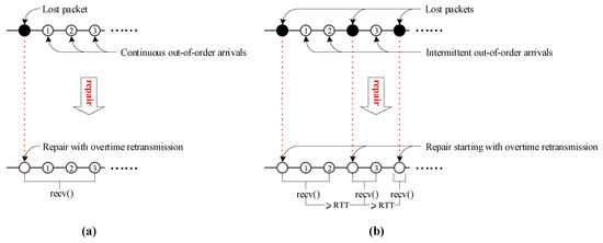
Figure 4.
Overtime loss event scenario. (a) Continuous out-of-order arrivals; (b) Intermittent out-of-order arrivals.
3.3. TCP Variants
Following the operation of IM-L-Rex, we can see that it estimates packet losses by retransmissions. As we know, for different TCP variants, different techniques are used to control TCP retransmissions. Therefore, the TCP variant in use is crucial to the accuracy of IM-L-Rex. Given this, this paper investigates the performance of IM-L-Rex under the following TCP variants:
- Reno: According to RFC 2581 [24], it cooperates with TCP’s basic congestion control mechanisms (e.g., slow start, congestion avoidance, fast recovery, etc.) to repair packet losses with overtime retransmissions and fast retransmissions.
- NewReno: This version, described in RFC 2582 [25], is an extension to the Reno. It mainly improves TCP’s fast recovery algorithm to avoid multiple retransmission timeouts in Reno’s fast recovery phase.
- SACK: It uses the Selective Acknowledgment (SACK) blocks to acknowledge out-of-order segments that arrived at the receiver and were not covered by the acknowledgement number. The SACK combines with a selective retransmission policy at the sender-side to repair packet losses and reduce spurious retransmissions. More details about SACK are available from RFC 2018 [26].
3.4. Summary
In this section, we detailed IM-L-Rex. Since IM-L-Rex is an evolution of L-Rex, to better understand it, we outline the differences between the two technologies as follows:
- (1)
- As the key parameters, RTT, H and K are all static in L-Rex, i.e., RTT is the time required for the connect() system call to complete, while the parameters H and K were optimized from repeated experiments on Asymmetric Digital Subscriber Lime (ADSL) and fast Ethernet, with values of 0.7 and 1%, respectively. On the contrary, the parameters RTT and K are dynamically estimated in IM-L-Rex by leveraging the TCP’s self-clocking mechanism. Moreover, the parameter H used for smoothing RTT is no longer needed in IM-L-Rex due to the dynamically estimated RTT.
- (2)
- Compared with L-Rex, IM-L-Rex is also committed to excluding the adverse effect of packet reordering by refining overtime retransmissions and fast retransmissions.
4. Implementation
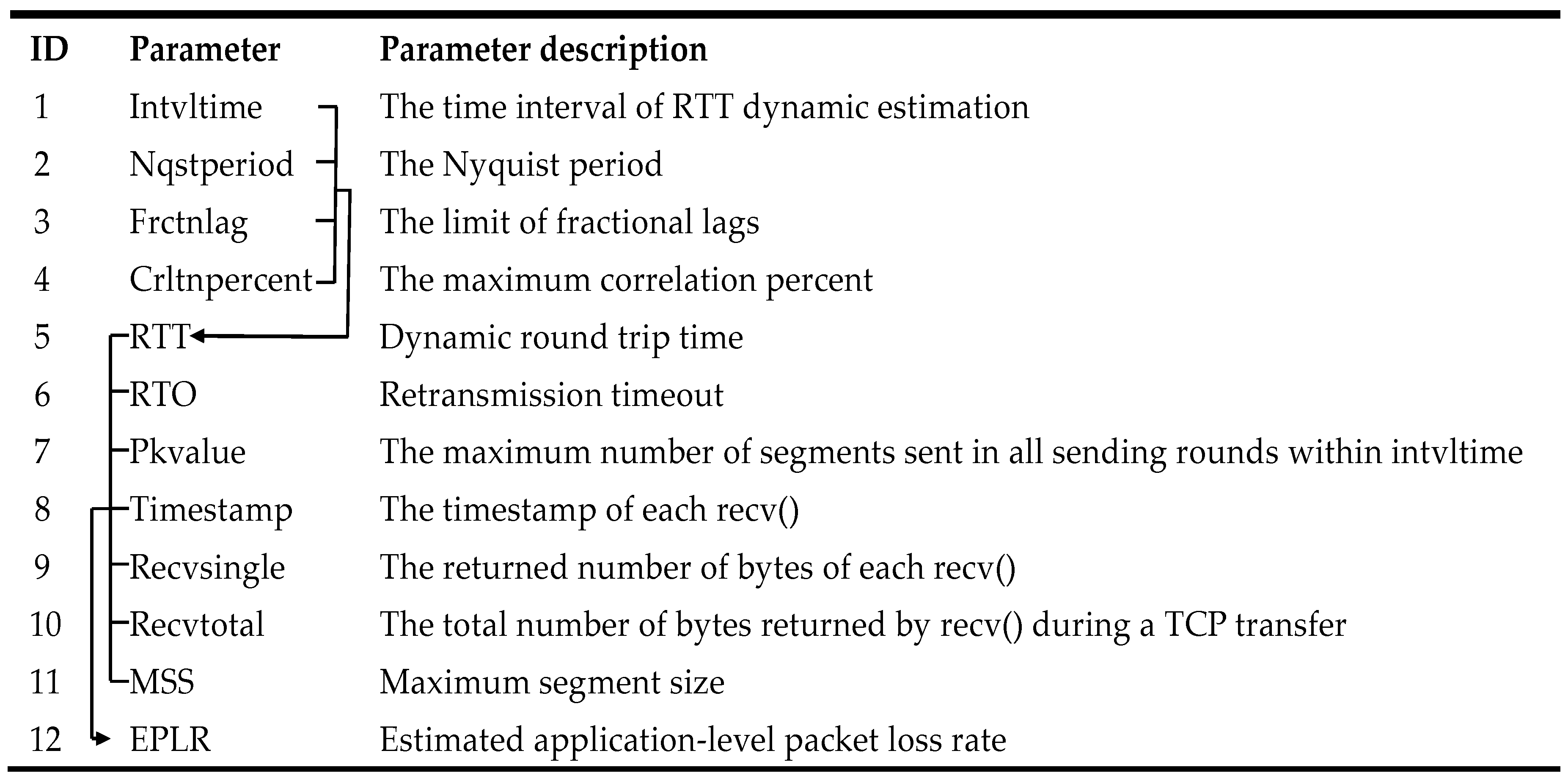
After an overview of IM-L-Rex, in the section, we systematically introduce its packet loss detection process. The parameters involved in IM-L-Rex are shown in Table 1. Among them, the first four parameters are used to dynamically determine RTT, and the parameters numbered 5 to 11 are used to estimate the application-level loss rate.

Table 1.
Description of parameters involved in improved L-Rex (IM-L-Rex).
Follow the loss detection process shown in Figure 5, we implemented IM-L-Rex. Specifically, within the time interval Intvltime (500 ms), the self-clocking-based RTT estimation firstly operates on the data sequence formed by the arriving recv()s to get the dynamic RTT. To improve the RTT estimation accuracy, the parameters Nqstperiod, Frctnlag, and Crltnpercent are used to exclude the negative effects. Among them, Nyquist is used for correcting the small lags caused by the noises like competing traffic, back-to-back received packets, and other network conditions disrupting the burst-gap patterns. In our implementation, the lags less than min(Nyquist period, 10 ms) are not considered. Frctnlag and Crltnpercent are set to 1/4 and 75% to exclude the effect of strong autocorrelation at multiples of the RTT. Furthermore, when estimating RTT, the parameters RTO and K deduced from Pkvalue are also obtained synchronously. Then, for the data returned by each recv(), we determine whether it indicates a likely retransmission by using the parameters Timestamp, RTT, and K. If it does, we further determine whether it indicates a packet loss by means of the relevant parameters RTT, Recvsingle, and RTO (i.e., the parameters RTT and Recvsingle for fast loss event, and the parameters RTT and RTO for overtime loss event). After that, we divide the total number of packets (Recvtotal/MSS) by the estimated number of packet losses (Lossnum++) to get the EPLR. Finally, the algorithm IM-L-Rex is shown in Algorithm 1.
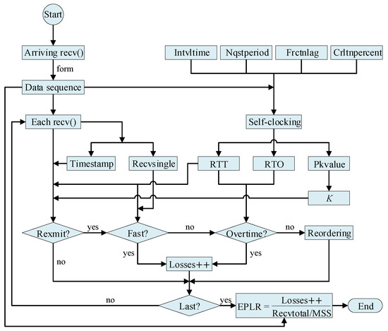
Figure 5.
Loss detection process of IM-L-Rex.
| Algorithm 1: IM-L-Rex |
| 01. //Preprocessing stage 02. Total_num = Loss_num = Nqst = EPLR = 0 03. Intvl = 500 04. Frctn = 1/4 05. Crltn = 0.75 06. S = null 07. for Recvdata returned by each recv() 08. //Form data sequence 09. Recvdata.addArray(S) 10. Total_num += Recvdata.getPktnum() 11. end for 12. for Recvdata in S 13. //Count application level traffic losses 14. if Recvdata.isRexmit(S, Intvl, Nqst, Frctn, Crltn) 15. if Recvdata.isFast(S, Intvl, Nqst, Frctn, Crltn) 16. Loss_num+=1 17. else if Recvdata.isFast(S, Intvl, Nqst, Frctn, Crltn) 18. Loss_num+=1 19. else 20. continue 21. else 22. continue 23. end for 24. EPLR = Loss_num / Total_num |
5. Experiments
In this section, we test IM-L-Rex with real measured data and testbed measurements. Among them, the real measured data obtained through controlled TCP transfers are used to verify the effectiveness of dynamic parameters, while the testbed measurements are performed to analyze the impact of packet reordering, TCP variants, and parameters RTT and K.
5.1. Controlled TCP Transfers
In order to focus on the model itself, the semantically complete TCP transfers are used to evaluate IM-L-Rex, where semantically complete TCP transfer is defined as a TCP transfer for which one can see the connection set-up (SYN-ACK) and another connection tear-down (FIN-ACK). Accordingly, the controlled TCP transfer (called “controlled TCP transfer” because we had full control over the two communicating end-hosts) shown in Figure 6 is used to produce the wanted semantically complete TCP transfer. In our previous work [12], we implemented controlled TCP transfer for research purposes. Specifically, our experiments involved four servers (see Table 2 for configuration information) within JSERNET and ten client hosts in the outside of JSERNET. JSERNET (Jiangsu Education and Research Network) is a regional academic network of China Education and Research Network (CERNET), and it covers more than 100 research units and universities. In January 2006, its backbone bandwidth increased from OC-48 to OC-192. In Table 2, hosts No. 1 to No. 3 are communication servers and are used for conducting controlled TCP transmissions with clients to form the required TCP streams, while host No. 4 is a storage server that stores the packet traces captured from the two communicating end-hosts. The controlled TCP transfer at the client side is realized with the Flow_Mirror, the tool that we developed and maintain [27]. Moreover, to fully evaluate the accuracy of IM-L-Rex, we placed some files of varied sizes on each communication server, and irregularly scheduled an Hyper Text Transfer Protocol based (HTTP-based) file transfer (that is, the client tool Flow_Mirror obtains the resource identified by the Uniform Resource Locator (URL) from the server with an HTTP GET request) between randomly chosen communication server and client host to obtain the TCP transfers with different sizes and various loss rates. During transfer, we used the sniffers (TCPDUMP on the sever side and WireShark on the client side) to collect packet traces from two endpoints of a TCP connection and compared the data packets to obtain the (Real Packet Loss Rate) RPLR.
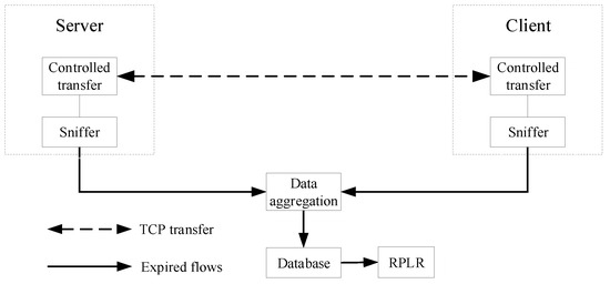
Figure 6.
Controlled TCP transfer architecture.

Table 2.
Server configuration information.
Notably, when validating L-Rex, Basso et al. used retransmissions to approximate RPLR. Although the retransmitted data pkts is a good approximation of packet losses, the spurious retransmissions caused by flaws in TCP’s retransmission schemes [14] make the retransmissions larger than the actual packet losses. Given this, in this paper, we get the real packet losses by comparing the packet traces at two communicating end-hosts [12]. Again, for the data packet performing IP fragmentation [28], as long as one fragment belonging to it is lost, the entire data packet is considered lost. In addition, the involved models in this paper are all based on application layer data. Thus, it is not enough to just capture the packet traces for calculating RPLR. To obtain the required data, during a TCP transfer, we also synchronously record the number of bytes returned by each recv() and the time elapsed since the previous recv(), as well as the values returned by other system calls, such as getsockopt() and connect(). Finally, the dataset EVLT_SET for evaluating IM-L-Rex is shown in Table 3. As we can see, three sizes of file transfers (1 Mbytes, 10 Mbytes, and 100 Mbytes) were chosen to evaluate the performance of IM-L-Rex when facing short and long TCP flows. Moreover, for rigorous evaluation, the practically relevant loss rate parameter space was also divided into three intervals ([0, 10−4), (10−4, 10−3), and (10−3, ∞)) to compare the performance of IM-L-Rex under different loss rates. In Table 3, the first row is the information of TCP flows with loss rate greater than 10−3, totaling 195 TCP transfers, while the second row is the information of the loss rate between 10−4 and 10−3, totaling 308 TCP transfers, and the third row is the results of the loss rate lower than 10−4, totaling 257 TCP transfers. The first column is the TCP transfers with file size of 1 MB, and the numbers of such TCP transfers corresponding to each loss rate interval are 57 (19%), 111 (37%), and 132 (44%), respectively, while the second column is the TCP transfers with file size of 10 MB, and the numbers of such TCP transfers corresponding to each loss rate interval are 68 (36%), 109 (42%), and 83 (32%), respectively, and the third column is the TCP transfers with file size of 100 MB, and the numbers of such TCP transfers corresponding to each loss rate interval are 70 (35%), 88 (44%), and 42 (21%), respectively.

Table 3.
EVLT_SET.
Figure 7 shows the empirical cumulative distribution function (CDF) of the relative errors of L-Rex and IM-L-Rex, for different size files and RPLR ranges. From Figure 7, we can see that L-Rex is more accurate under low RPLR than it is under high RPLR. This can be attributed to the fact that L-Rex was designed and optimized for landline network with moderate losses (i.e., RPLR ≥ 10−4). In addition, we can see that, when the RPLR is on the same order of magnitude, the estimation accuracy of L-Rex becomes lower as the file size increases. This can be explained by the fact that L-Rex takes the time required for the connect() system call to complete as RTT, while the RTT at the TCP connection establishment is usually inconsistent with that after the transmission is stable. It can be inferred that, when the file is large, the fluctuation of RTT is larger, which makes the estimation accuracy of L-Rex face more severe challenges. On the contrary, benefiting from dynamic parameters, in Figure 7, IM-L-Rex is more accurate than L-Rex and is basically not affected by packet loss rate and file size.
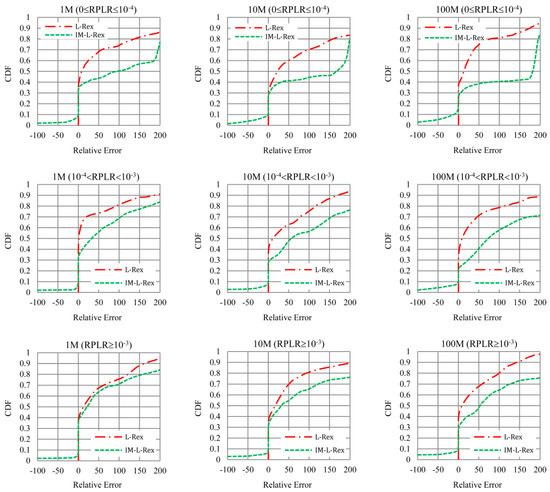
Figure 7.
Cumulative distribution function (CDF) of the relative errors of L-Rex and IM-L-Rex.
L-Rex is designed and optimized based on fast Ethernet and ADSL. As we know, ADSL is rarely used nowadays. Correspondingly, the experimental results in Figure 7 are all derived from the TCP transfers whose clients are located in fast Ethernet. To verify the performance of IM-L-Rex in other current mainstream access networks, we also compared L-Rex and IM-L-Rex in gigabit Ethernet. For the sake of highlighting the advantages of L-Rex, we chose TCP transfers with a file size of 1 MB and a packet loss rate greater than 10−3, for experimental comparison. From the result in Figure 8, we can see that the accuracy of L-Rex in gigabit Ethernet is worse than that in fast Ethernet. The error mainly stems from the limitations of the static parameters optimized in ADSL and fast Ethernet, i.e., in gigabit Ethernet; the difference in the number of bytes received by each recv() is higher than that assumed by L-Rex. In this case, the parameter values of 1% and 0.7 may be too strict. In comparison, in Figure 8, the accuracy of IM-L-Rex based on dynamic parameters is comparable to that in fast Ethernet and is not affected by the specific level 2 connection type.
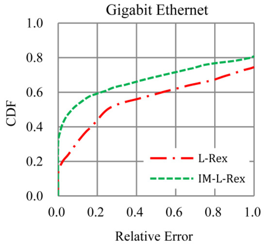
Figure 8.
Result of gigabit Ethernet.
5.2. Testbed
5.2.1. Impact of Packet Reordering
In this subsection, we use testbed measurements to investigate the performance of IM-L-Rex in processing packet reordering. The testbed shown in Figure 9 consisted of three fedora8 virtual machines installed on the fedora17 operating system: host A, host B, and router R. We used GNU Zebra to emulate and configure the router, while the packet reordering and random packet losses are added to network interface eth1 with Netem. Corresponding to the scenario in Figure 9, the specific testbed parameters are shown in Table 4. In the previous experiments, we verified the performance of IM-L-Rex under fast Ethernet and gigabit Ethernet, while here the link bandwidth is set to 10 Mbps to further verify the robustness of IM-L-Rex under lower bandwidth. Also, the 10-second random-data TCP download is consistent with the fact that most application level tools run their tests for a fixed number of seconds (typically 10) [7].

Figure 9.
Testbed scenario.

Table 4.
Testbed parameters.
The simulation results of L-Rex and IM-L-Rex under different reordering rate (the proportion of data packets reordered during a TCP transfer) are shown in Figure 10. The application-level packet loss rate, in the actual network, typically spans several orders of magnitude. Accordingly, in the final experiment results, five to 10 TCP transfer samples were selected for each order of magnitude to investigate the effectiveness of our strategy used for excluding packet reordering. In Figure 10, the dashed bisector line represents the exact prediction, and the closer the points are to the bisection, the more accurate the corresponding model is. From Figure 10, we can see that, on the whole, the points of L-Rex are scattered on both sides of the bisection, while the points of IM-L-Rex are mainly located above the bisection and are closer to the bisection than L-Rex. Moreover, we can see that, as the proportion of packets that suffer reordering increases, L-Rex becomes less accurate, while IM-L-Rex is relatively accurate. All this indicates that our strategy is effective; in other words, IM-L-Rex is more robust than L-Rex in the face of packet reordering. Meanwhile, the points scattered on both sides of the bisection imply that L-Rex sometimes overestimates and sometimes underestimates, while the points above the bisection indicate that IM-L-Rex will produce overestimates in most cases. The phenomenon behind L-Rex further illustrates that the static parameters of L-Rex are unable to adapt to the dynamic and complex network conditions. As for the reason why IM-L-Rex always outputs overestimates is that IM-L-Rex also utilizes retransmissions to realize loss estimation; although the estimation of IM-L-Rex is closer to the actual number of retransmissions, the spurious retransmissions included in retransmissions inevitably skewed the estimation of IM-L-Rex and produced the overestimates. Moreover, the results in Figure 10 also show that L-Rex performs poorly at low RPLR, which may be owing to the static parameter values (i.e., 1% for H and 0.7 for K) optimized under moderate losses.
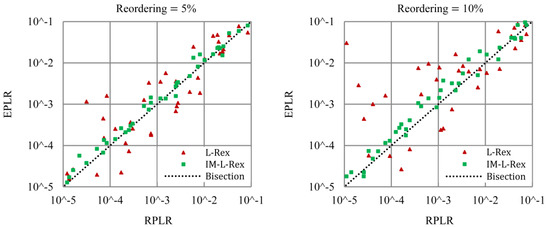
Figure 10.
The performance of IM-L-Rex and L-Rex in processing packet reordering.
5.2.2. Impact of TCP Variants
In order to check how TCP variant influences the proposal, we carried out experiments with the same set-up shown in Figure 9 to compare the performance of IM-L-Rex and L-Rex under different TCP variants (i.e., Reno, NewReno, and SACK). Unlike the parameters in Table 1, we did not add packet reordering to the network interface to focus on the effect of the TCP variant itself. In Figure 11, the experiment results can be seen. It can be seen that, regardless of IM-L-Rex or L-Rex, in terms of overall estimation accuracy, SACK is best, NewReno is second, and Reno is the worst. Particularly, we can see that, although IM-L-Rex outperforms L-Rex under the same TCP variant, IM-L-Rex is not always superior to L-Rex in the entire parameter space. That is, the L-Rex under SACK is better than the IM-L-Rex under Reno when the relative error is greater than 66.43%. From these, it is inferred that different TCP variants have a great impact on the performance of IM-L-Rex.
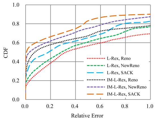
Figure 11.
Impact of TCP variants.
Exploring the reasons behind this phenomenon, we found that it is related to the different mechanisms via which different TCP variants handle packet losses. Specifically, NewReno and Reno have the same mechanism in dealing with a single packet loss. However, when losing multiple packets at a time, NewReno shows its advantages by reducing the occurrence of overtime retransmissions with the improved fast-recovery algorithm. Likewise, compared with NewReno, SACK utilizes SACK blocks to reduce spurious retransmissions, thus showing its advantages in dealing with packet losses. Furthermore, since IM-L-Rex and L-Rex are based on retransmissions, the relative advantages between different TCP variants ultimately lead to their different performance.
5.2.3. Impact of Parameters RTT and K
To fully evaluate IM-L-Rex, we also investigated the effects of dynamic RTT and dynamic K on IM-L-Rex. The evaluation data come from the TCP transfers under NewReno version in Section 5.2.2, and the experiment results are shown in Figure 12. Comparing L-Rex and “IM-L-Rex, Dynamic RTT, Static K”, we can see that the dynamic RTT has a certain improvement for the estimation accuracy of L-Rex. Similarly, the comparison of “IM-L-Rex, Dynamic RTT, Static K” and L-Rex also illustrates that the dynamic K has a certain improvement for the estimation accuracy of L-Rex, but its improvement effect is less than that of dynamic RTT. This indicates that, for IM-L-Rex, RTT is a more critical parameter than K, which has the more important role in the estimation accuracy.
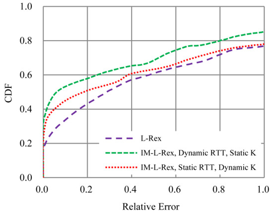
Figure 12.
Impact of parameters RTT and K (“IM-L-Rex, Dynamic RTT, Static K” represents the IM-L-Rex taking dynamic RTT and static K, while “IM-L-Rex, Static RTT, Dynamic K” represents the IM-L-Rex taking static RTT and dynamic K).
Nonetheless, it is worth pointing out that, although IM-L-Rex is superior to L-Rex, there is still a gap between the estimation accuracy and the practical application requirement [29]. From our experiments, we can see that some relative errors are even higher than 100% for both IM-L-Rex and L-Rex. Upon tracing its root, for IM-L-Rex, the estimation errors mainly stem from the inevitably spurious retransmissions associated with the flaws in TCP’s retransmission schemes. Accordingly, for our future work, further excluding the effect of spurious retransmissions is necessary and crucial to eliminate the gap.
6. Conclusion and Future Work
Faced with the packet dynamics along the network path, dynamic parameters are beneficial to improve the accuracy and robustness of the model L-Rex. To this end, we leveraged the TCP’s self-clocking mechanism to dynamically estimate the parameters required by L-Rex. Meanwhile, the effect of packet reordering was also considered by refining fast retransmissions and overtime retransmissions. Correspondingly, the experiments performed with real measured data and testbed measurements showed that the approach and strategy proposed in this paper are effective. Yet, from the experimental results, it can be also seen that, although IM-L-Rex is superior to L-Rex in terms of estimation accuracy and stability, there is still a gap between the estimation accuracy and the practical application requirement. With our analysis, spurious retransmission is the root of the problem. Also, minimally, PLR would vary randomly in real network; thus, coping with this problem will be beneficial to improve the robustness of IM-L-Rex. To this end, for our future work, we intend to further mine the information available from the application layer to exclude these adverse effects. Moreover, since wireless access networks are now very popular and have noticeable effects on packet losses and RTT, testing IM-L-Rex in wireless networks will be interesting.
Author Contributions
Conceptualization, H.L. and W.D.; data curation, H.L.; investigation, H.L.; methodology, H.L.; resources, H.L.; software, H.L. and L.D.; validation, H.L.; visualization, H.L.; writing—original draft, H.L.; writing—review and editing, W.D.; project administration, W.D.
Funding
This research was funded by the National Nature Science Foundation of China (No. 61602114), the National Nature Science Foundation of China (No. 60973123), and CERNET Innovation Project (No. NGII20170406).
Conflicts of Interest
The authors declare no conflict of interest.
References
- Antonopoulos, A.; Kartsakli, E.; Perillo, C.; Verikoukis, C. Shedding light on the Internet: Stakeholders and network neutrality. IEEE Commun. Mag. 2017, 55, 216–223. [Google Scholar] [CrossRef]
- Peitz, M.; Schuett, F. Net neutrality and inflation of traffic. Int. J. Ind. Organ. 2016, 46, 16–62. [Google Scholar] [CrossRef]
- Bauer, J.M.; Knieps, G. Complementary innovation and network neutrality. Telecommun. Policy 2018, 42, 172–183. [Google Scholar] [CrossRef]
- Dustdar, S.; Duarte, E.P. Network Neutrality and Its Impact on Innovation. IEEE Internet Comput. 2018, 22, 5–7. [Google Scholar] [CrossRef]
- Schulzrinne, H. Network Neutrality Is About Money, Not Packets. IEEE Internet Comput. 2018, 22, 8–17. [Google Scholar] [CrossRef]
- Statovci-Halimi, B.; Franzl, G. QoS differentiation and Internet neutrality. Telecommun. Syst. 2013, 52, 1605–1614. [Google Scholar] [CrossRef]
- Basso, S.; Meo, M.; Servetti, A.; De Martin, J.C. Estimating packet loss rate in the access through application-level measurements. In Proceedings of the ACM SIGCOMM workshop on Measurements up the stack, Helsinki, Finland, 17 August 2012; pp. 7–12. [Google Scholar]
- Basso, S.; Meo, M.; De Martin, J.C. Strengthening measurements from the edges: Application-level packet loss rate estimation. ACM SIGCOMM Comput. Commun. Rev. 2013, 43, 45–51. [Google Scholar] [CrossRef]
- Ellis, M.; Pezaros, D.P.; Kypraios, T.; Perkins, C. A two-level Markova model for packet loss in UDP/IP-based real-time video applications targeting residential users. Comput. Netw. 2014, 70, 384–399. [Google Scholar] [CrossRef]
- Baglietto, M.; Battistelli, G.; Tesi, P. Packet loss detection in networked control systems via process measurements. In Proceedings of the IEEE Conference on Decision and Control, Miami Beach, FL, USA, 17–19 December 2018; pp. 4849–4854. [Google Scholar]
- Mittag, G.; Möller, S. Single-ended packet loss rate estimation of transmitted speech signals. In Proceedings of the IEEE Global Conference on Signal and Information Processing, Anaheim, CA, USA, 26–29 November 2018; pp. 226–230. [Google Scholar]
- Lan, H.; Ding, W.; Gong, J. Useful Traffic Loss Rate Estimation Based on Network Layer Measurement. IEEE Access 2019, 7, 33289–33303. [Google Scholar] [CrossRef]
- Carra, D.; Avrachenkov, K.; Alouf, S.; Blanc, A.; Nain, P.; Post, G. Passive online RTT estimation for flow-aware routers using one-way traffic. In Proceedings of the 9th International IFIP TC 6 Networking Conference, Chennai, India, 11–15 May 2010; pp. 109–121. [Google Scholar]
- Allman, M.; Eddy, W.M.; Ostermann, S. Estimating loss rates with TCP. ACM SIGMETRICS Perform. val. Rev. 2003, 31, 12–24. [Google Scholar] [CrossRef]
- Priya, S.; Murugan, K. Improving TCP performance in wireless networks by detection and avoidance of spurious retransmission timeouts. J. Inf. Sci. Eng. 2015, 31, 711–726. [Google Scholar]
- Anelli, P.; Lochin, E.; Harivelo, F.; Lopez, D.M. Transport congestion events detection (TCED): Towards decorrelating congestion detection from TCP. In Proceedings of the ACM Symposium on Applied Computing, Sierre, Switzerland, 22–26 March 2010; pp. 663–669. [Google Scholar]
- Zhani, M.F.; Elbiaze, H.; Aly, W.H.F. TCP based estimation method for loss control in OBS networks. In Proceedings of the IEEE GLOBECOM, Honolulu, HI, USA, 30 November–4 December 2009; pp. 1–6. [Google Scholar]
- Ullah, S.; Ullah, I.; Qureshi, H.K.; Haw, R.; Jang, S.; Hong, C.S. Passive packet loss detection in Wi-Fi networks and its effect on HTTP traffic characteristics. In Proceedings of the International Conference on Information Networking, Phuket, Thailand, 10–12 February 2014; pp. 428–432. [Google Scholar]
- Hagos, D.H.; Engelstad, P.E.; Yazidi, A.; Kure, Ø. A machine learning approach to TCP state monitoring from passive measurements. In Proceedings of the IEEE Wireless Days, Dubai, UAE, 3–5 April 2018; pp. 164–171. [Google Scholar]
- Laghari, A.A.; He, H.; Channa, M.I. Measuring effect of packet reordering on quality of experience (QoE) in video streaming. 3D Research 2018, 9, 30. [Google Scholar] [CrossRef]
- Veal, B.; Li, K.; Lowenthal, D. New methods for passive estimation of TCP round-trip times. In International Workshop on Passive and Active Network Measurement; Springer: Berlin/Heidelberg, Germany, 2005; pp. 121–134. [Google Scholar]
- Mirkovic, D.; Armitage, G.; Branch, P. A survey of round trip time prediction systems. IEEE Commun. Surv. Tutor. 2015, 20, 1758–1776. [Google Scholar] [CrossRef]
- Paxson, V.; Allman, M.; Chu, J.; Sargent, M. Computing TCP’s retransmission timer. RFC 6298. 2011. [Google Scholar] [CrossRef]
- Allman, M.; Paxson, V.; Stevens, W. TCP Congestion Control, RFC 2581. 1999. [Google Scholar] [CrossRef]
- Floyd, S.; Henderson, T. The NewReno Modification to TCP's Fast Recovery Algorithm, RFC 2582. 1999. [Google Scholar] [CrossRef]
- Mathis, M.; Mahdavi, J.; Floyd, S.; Romanow, A. TCP Selective Acknowledgment Options, RFC 2018. [CrossRef]
- Lan, H.; Ding, W.; Zhang, Y. Passive overall packet loss estimation at the border of an ISP. KSII T. Internet. Inf. 2018, 12, 3150–3171. [Google Scholar]
- Stevens, W.R. TCP/IP Illustrated, Volume 1: The protocols, 1st ed.; Addison-Wesley Publisher: Boston, MA, USA, 1994; pp. 136–139. [Google Scholar]
- Nguyen, H.X.; Roughan, M. Rigorous statistical analysis of internet loss measurements. IEEE/ACM Trans. Netw. 2013, 21, 734–745. [Google Scholar] [CrossRef]
© 2019 by the authors. Licensee MDPI, Basel, Switzerland. This article is an open access article distributed under the terms and conditions of the Creative Commons Attribution (CC BY) license (http://creativecommons.org/licenses/by/4.0/).
