Article

Influence of Cattaneo–Christov Heat Flux on MHD Jeffrey, Maxwell, and Oldroyd-B Nanofluids with Homogeneous-Heterogeneous Reaction

1
Department of Mathematics, Abdul Wali Khan University Mardan, Mardan 23200, Pakistan
2
Department of Mathematics, Qurtuba University of Science and Information Technology, Peshawar 25000, Pakistan
3
KMUTTFixed Point Research Laboratory, Room SCL 802 Fixed Point Laboratory, Science Laboratory Building, Department of Mathematics, Faculty of Science, King Mongkut’s University of Technology Thonburi (KMUTT), Bangkok 10140, Thailand
4
KMUTT-Fixed Point Theory and Applications Research Group, Theoretical and Computational Science Center (TaCS), Science Laboratory Building, Faculty of Science, King Mongkut’s University of Technology Thonburi (KMUTT), Bangkok 10140, Thailand
5
Department of Medical Research, China Medical University Hospital, China Medical University, Taichung 40402, Taiwan
6
Department of Mathematics, Kohat University of Science and Technology, Kohat 26000, Pakistan
*
Author to whom correspondence should be addressed.
Symmetry 2019, 11(3), 439; https://doi.org/10.3390/sym11030439
Submission received: 4 March 2019 / Revised: 17 March 2019 / Accepted: 19 March 2019 / Published: 25 March 2019
(This article belongs to the Special Issue Symmetry and Fluid Mechanics)

Abstract

:
This research article deals with the determination of magnetohydrodynamic steady flow of three combile nanofluids (Jefferey, Maxwell, and Oldroyd-B) over a stretched surface. The surface is considered to be linear. The Cattaneo–Christov heat flux model was considered necessary to study the relaxation properties of the fluid flow. The influence of homogeneous-heterogeneous reactions (active for auto catalysts and reactants) has been taken in account. The modeled problem is solved analytically. The impressions of the magnetic field, Prandtl number, thermal relaxation time, Schmidt number, homogeneous–heterogeneous reactions strength are considered through graphs. The velocity field diminished with an increasing magnetic field. The temperature field diminished with an increasing Prandtl number and thermal relaxation time. The concentration field upsurged with the increasing Schmidt number which decreased with increasing homogeneous-heterogeneous reactions strength. Furthermore, the impact of these parameters on skin fraction, Nusselt number, and Sherwood number were also accessible through tables. A comparison between analytical and numerical methods has been presented both graphically and numerically.

1. Introduction

A fluid composed of nanoparticles is called nanofluid. Nanoparticles of materials such as metallic oxides, carbide ceramics, nitride metals, ceramics, semiconductors, single, double or multi walled carbon nanotubes, alloyed, nanoparticles, etc. have been used for the preparation of nanofluids. Nanofluids have many characteristics in heat transfer, including microelectronics, local refrigerator, cooler, machining, and heat exchanger. The idea of nanofluid was introduced by Choi [1]. The Fourier’s [2] recommended law of heat conduction normally works for heat transmission features from the time it was presented in the literature. By including the relaxation time parameter Cattaneo [3] it has improved this law and this term overwhelms the paradox of heat conduction. Christov [4] has named this theory Cattaneo-Christov heat flux theory, by further modifying the Cattaneo theory by exchanging the time derivative with Oldroyd-B upper convicted derivative. Mustafa [5] scrutinized the model [4] for heat transmission in a rotating Maxwell nanofluid flow. Chen [6] probed the influence of heat transfer and viscous dissipation of nanofluid flow over a stretching sheet. Sheikholeslami et al. [7,8,9,10,11] deliberated the three-dimensional magnetohydrodynamics (MHD) nanofluid flow in parallel rotating plates. Sheikholeslami [11,12,13,14,15] analytically and numerically deliberated the applications of nanofluids with different properties, behavior, and influences. Dawar et al. [16] examined the flow Williamson nanofluid over a stretching surface. Shah et al. [17] examined the micropolar nanofluid flow in rotating parallel plates with Hall current impact. Maleki et al. [18] scrutinized the non-Newtonian nanofluids flow and heat transfer over a porous surface. Nasiri et al. [19] deliberated the smoothed particle by a hydrodynamics approach for numerical simulation of nanofluid flows. Rashidi et al. [20] used the nanofluids in a circular tube heat exchanger and examined the entropy generation. Safaei et al. [21] studied numerically and experimentally the nanofluids convective heat transfer in closed conduits. Mahian et al. [22,23] presented the advances in the simulation and modeling of the flows of nanofluids.
Due to its relaxation properties, Jeffrey, Maxwell, and Oldroyd-B nanofluids have significant applications in the area of fluid mechanics. Ahmad et al. [24] scrutinized the flow of Jeffrey nanofluid with Magnetohydrodynamic impact. Ahmad and Ishak [25] deliberated the flow of Jeffrey nanofluid with MHD and transverse magnetic field impacts in a porous medium. Hayat et al. [26] probed the Oldroyd-B nanofluid flow with heat transfer and thermal radiation impacts. Raju et al. [27] deliberated the flow of Jeffrey nanofluid with a homogenous-heterogeneous reaction and non-linear thermal radiation impacts. The articles that are related to Jeffrey nanofluid can be found in [28,29,30,31,32]. Hayat et al. [33] inspected the MHD Maxwell nanofluid flow using suction/injection. Raju et al. [34] presented the heat and mass transmission in three-dimensional non-Newtonian nanofluid and Ferrofluid. Sandeep and Sulochana [35] investigated the mixed convection micropolar nanofluid flow over a stretching sheet. Raju et al. [36] deliberated the impacts of an inclined magnetic field, thermal radiation and cross diffusion on the two-dimensional flow. Nadeem et al. [37] presented the heat and mass transfer in Jeffrey nanofluid. Makinde et al. [38] deliberated the unsteady fluid flow with convective boundary conditions. Sheikholeslami [39] discussed the hydro-thermal behavior of nanofluids flow because of its external heated plates. Shah et al. [40] presented the Darcy-Forchheimer flow of radiative carbon nanotubes in a rotating frame. Chai et al. [41] presented a review of the heat transfer and hydrodynamic characteristics of nano/microencapsulated phase. Shah et al. [42] examined the electro-magneto micropoler Casson Ferrofluid over a stretching/shrinking sheet. Dawar et al. [43] analyzed the MHD CNTs Casson nanofluid in rotating channels. Khan et al. [44] deliberated the Williamson nanofluid flow over a linear stretching surface. Imtiaz et al. [45] examined the unsteady MHD flow due to a curved stretchable surface with homogeneous–heterogeneous reactions. Hayat et al. [46] deliberated the flow of nanofluids with homogeneous–heterogeneous reaction impacts over a non-linear stretched sheet with variable thickness. The recent study about nanofluid with application can be seen [47,48,49,50].
The present work is based on an analysis of MHD flow of three combine nanofluids (Maxwell, Oldroyd-B, and Jeffrey) over a linear stretching surface. The present model composed of Cattaneo–Christov heat flux. The impact of homogeneous-heterogeneous reactions were taken in this model. A boundary layer methodology was used in the mathematical expansion. The impact of dimensionless parameters on the fluid flow have been presented through graphs and tables.

2. Mathematical Modeling and Formulation

The incompressible electrically conducted three combined nanofluids (Jeffrey, Maxwell, and Oldroyd-B) were confined by a linear stretched surface. The fluid flow was taken in a two-dimensional steady state with stable surface temperature. x -axis was considered parallel to the surface, while y -axis was orthogonal to x -axis in the chosen coordinate system. The stretching velocity in x -axes direction was defined as U w ( x ) = ζ x . The conclusion of homogeneous-heterogeneous reactions on the fluid flows of two chemical species I and J were taken in account. In the y -axis direction a uniform magnetic field B 0 was acting. The heat transmission procedure was applied through Cattaneo–Christov heat flux theory.
In case of cubic autocatalysis, the Homogeneous reaction is [45,46]
I + 2 J 3 J , r a t e = k c i j 2 ,
While on the catalyst surface, the heterogeneous reaction has been defined by
I J , r a t e = k s i ,
where k c , k s , I , J , i , j are the rate constants, chemical species, and concentrations of chemical species, respectively.
In the absence of viscous dissipation and thermal radiation, the boundary layer equations leading to the flow of viscoelastic fluids can be written as follows [47]:
u x + v y = 0 ,
u u x + v u y = λ 1 ( u 2 u x x + 2 u v u x y + v 2 u y y ) + υ f 1 + λ 2 { u y y + λ 3 ( u u x y y + u y u x y + υ u y y y u x u y y ) } σ B 0 2 ρ f u ,
ρ c p ( u T x + v T y ) = . q ,
u i x + v i y = D I i y y k c i j 2 ,
u j x + v j y = D J j y y + k c i j 2 .
Here u , v , μ , ρ f , υ f are velocity components in their respective directions, dynamic viscosity, density, and kinematic viscosity respectively. λ 1 , λ 2 , λ 3 are the relaxation time, a proportion of the relaxation to retardation times, respectively. T , σ f , B 0 indicated the temperature, electrical conductivity and the transverse magnetic field.
The problem is studied based on the following conditions:
  • Oldroyd-B nanofluid when λ 1 0 , λ 2 = 0   and   λ 3 0 .
  • Maxwell nanofluid when λ 1 0 , λ 2 = 0   and   λ 3 = 0 .
  • Jeffrey nanofluid when λ 1 = 0 , λ 2 0   and   λ 3 0 .
The heat flux theory which was presented by Cattaneo–Christov:
q + λ 1 { q t + V q q V + ( V ) q + q t } = k T ,
where k , q represented thermal conductivity and heat flux. Classical Fourier’s law was assumed by setting λ 1 = 0 in Equation (8). By assuming the condition ( . V = 0 ) and steady flow with ( q t = 0 ) , Equation (8) became:
q + λ 1 ( V . q q . V ) = k T .
The heat transfer equation proceeded as:
u T x + v T y + λ 1 Φ E = α ( T y y ) ,
where Φ E is given as:
Φ E = u u x T x + v v y T y + u v x T y + v u y T x + 2 u v T x y + u 2 T x x + v 2 T y y .
The accompanying boundary conditions were:
u = U w ( x ) = ζ x , v = 0 , T = T w , D I i y = k s i , D J j y = k s i   at   y = 0 , u 0 ,   T T , i i 0 , j 0   at   y ,
where α = k ρ c p indicated the thermal diffusivity, D I and D J indicated the diffusion coefficients, T w denoted the temperature at the surface, T for the surrounding fluid temperature and ζ for non-negative stretching rate constant with T 1 as the dimension.
u = ζ x F ( η ) , v = ( ζ υ ) 1 2 F ( η ) , η = ( ζ υ ) 1 2 y , G ( η ) = T T T w T , i = i 0 ϕ ( η ) , j = i 0 h ( η ) .
Apparently the equation of continuity is satisfied and Equations (4)–(13) become:
F + κ 2 ( F 2 F F ) M ( 1 + λ 2 ) F ( 1 + λ 2 ) { F 2 F F + κ 1 ( F 2 F 2 F F F ) } = 0 ,
G + Pr { F G Ω ( F F G + F 2 G ) } = 0 ,
ϕ + S c ( F ϕ K ϕ h 2 ) = 0 ,
δ h + S c ( F h + K ϕ h 2 ) = 0 ,
with boundary conditions:
F = 0 , F = 1 , G = 1 , ϕ = K s ϕ , δ h = K s ϕ   at   ϖ = 0 , F 0 , G 0 , ϕ 1 , h 0   at   η ,
In the above equations, M = σ n f B 0 2 ρ f ζ indicated the magnetic field, κ 1 = λ 1 ζ   and   κ 2 = λ 3 ζ were the Debora numbers with respect to relaxation and retardation time, Pr = υ f α represented the Prandtl number, Ω = ζ λ 1 indicated the thermal relaxation time, S c = υ f D I is the Schmidt number, K = k c i 0 2 U w indicating the homogeneous reaction strength, K s = k s D I i 0 ζ υ f represented the heterogeneous reaction strength, and δ = D J D I indicated the diffusion coefficient, When D I = D J then δ = 1 and as a result:
ϕ ( η ) + h ( η ) = 1 .
Now Equations (16) and (17) yield:
ϕ + S c { F ϕ K ϕ ( 1 ϕ ) 2 } = 0 .
The subjected boundary conditions are:
ϕ ( 0 ) = K s ϕ ( 0 ) , ϕ ( ) 1 .
Skin friction coefficient through the dimensionless scale is:
Re x 1 2 C f x = ( 1 + κ 1 1 + κ 2 ) F ( 0 ) .
where Re x is called the local Reynolds number.
The dimensionless form of N u x and S h x were found as:
N u x = G ( 0 ) , S h x = ϕ ( 0 ) .

3. Solution by Homtopy Analysis Method (HAM)

To evaluate the Equations (14), (15) and (20) with boundary conditions (18) and (21) using HAM with the following procedure.
The initial assumptions were picked as below:
F ¯ 0 ( η ) = 1 e η ,   G ¯ 0 ( η ) = e η , ϕ ¯ 0 ( η ) = e η .
The linear operators were taken as L F ¯ , L G ¯   and   L ϕ ¯ :
L F ¯ ( F ¯ ) = F ¯ F ¯ , L G ¯ ( G ¯ ) = G ¯ G ¯ , L ϕ ¯ ( ϕ ¯ ) = ϕ ¯ ϕ ¯ ,
With the following properties:
L F ¯ ( r 1 + r 2 e η + r 3 e η ) = 0 ,   L G ¯ ( r 4 e η + r 5 e η ) = 0 , L ϕ ¯ ( r 6 e η + r 7 e η ) = 0 ,
where r i ( i = 1 7 ) were the constants:
The resulting non-linear operators N F ¯ , N G ¯ and N ϕ ¯ were specified as:
N F ¯ [ F ¯ ( η ; τ ) ] = 3 F ¯ ( η ; τ ) η 3 + κ 2 { ( 2 F ¯ ( η ; τ ) η 2 ) 2 F ¯ ( η ; τ ) η 4 F ¯ ( η ; τ ) 4 η } M ( 1 + λ 2 ) { ( F ¯ ( η ; τ ) η ) 2 F ¯ ( η ; τ ) 2 F ¯ ( η ; τ ) η 2 + κ 1 ( F ¯ 2 ( η ; τ ) 3 F ¯ ( η ; τ ) η 3 2 F ¯ ( η ; τ ) F ¯ ( η ; τ ) η 2 F ¯ ( η ; τ ) η 2 ) } ,
N G ˙ [ F ¯ ( η ; τ ) , G ¯ ( η ; τ ) ] = 2 G ¯ ( η ; τ ) η 2 + Pr { F ¯ ( η ; τ ) G ¯ ( η ; τ ) η Ω ( F ¯ ( η ; τ ) F ¯ ( η ; τ ) η G ¯ ( η ; τ ) η + F ¯ 2 ( η ; τ ) 2 G ¯ ( η ; τ ) η 2 ) } ,
N ϕ ¯ [ F ¯ ( η ; τ ) , ϕ ¯ ( η ; τ ) ] = 2 ϕ ¯ ( η ; τ ) η 2 + S c { F ¯ ( η ; τ ) ϕ ¯ ( η ; τ ) η K ( ϕ ¯ 3 ( η ; τ ) 2 ϕ ¯ 2 ( η ; τ ) + ϕ ¯ ( η ; τ ) ) } ,
The zeroth-order problem for Equations (14), (15) and (20) were:
( 1 τ ) L F ¯ [ F ¯ ( η ; τ ) F ¯ 0 ( η ) ] = τ F ¯ N F ¯ [ F ¯ ( η ; τ ) ] ,
( 1 τ ) L G ¯ [ G ¯ ( η ; τ ) G ¯ 0 ( η ) ] = τ G ¯ N G ¯ [ F ¯ ( η ; τ ) , G ¯ ( η ; τ ) ] ,
( 1 τ ) L ϕ ¯ [ ϕ ¯ ( η ; τ ) ϕ ¯ 0 ( η ) ] = τ ϕ ¯ N ϕ ¯ [ F ¯ ( η ; τ ) , ϕ ¯ ( η ; τ ) ] .
The related boundary conditions where:
F ¯ ( η ; τ ) | η = 0 = 0 ,   F ¯ ( η ; τ ) η | η = 0 = 1 ,   F ¯ ( η ; τ ) η | η = 0 ,   G ¯ ( η ; τ ) | η = 0 = 1 ,   G ¯ ( η ; τ ) | η = 0 , ϕ ¯ ( η ; τ ) η | η = 0 = K s ϕ ¯ ( η ; τ ) | η = 0 ,   ϕ ¯ ( η ; τ ) | η = 1 ,
where τ [ 0 , 1 ] is the embedding parameter, F ¯ ,   G ¯ , ϕ ¯ that were used to control the solution convergence. When τ = 0   and   τ = 1 we have:
F ¯ ( η ; 1 ) = F ¯ ( η ) ,   G   ¯ ( η ; 1 ) = G ¯ ( η )   and     ϕ ¯ ( η ; 1 ) = ϕ ¯ ( η ) ,
Expanding F ¯ ( η ; τ ) ,   G   ¯ ( η ; τ )   and   ϕ ¯ ( η ; τ ) by Taylor’s series:
F ¯ ( η ; τ ) = F ¯ 0 ( η ) + q = 1 F ¯ q ( η ) τ q ,   G ¯ ( η ; τ ) = G ¯ 0 ( η ) + q = 1 G ¯ q ( η ) τ q , ϕ ¯ ( η ; τ ) =   ϕ ¯ 0 ( η ) + q = 1 ϕ ¯ q ( η ) τ q .
where:
F ¯ q ( η ) = 1 q ! F ¯ ( η ; τ ) η | τ = 0 ,   G   ¯ q ( η ) = 1 q ! G ¯ ( η ; τ ) η | τ = 0 and   ϕ ¯ q ( η ) = 1 q ! ϕ ¯ ( η ; τ ) η | τ = 0 .
The F ¯ , G ¯   and   ϕ ¯ are taken in such a way that the series (35) converges at τ = 1 , we have:
F ¯ ( η ) = F ¯ 0 ( η ) + q = 1 F ¯ q ( η ) ,   G ¯ ( η ) = G ¯ 0 ( η ) + q = 1 G ¯ q ( η ) , ϕ ¯ ( η ) = ϕ ¯ 0 ( η ) + q = 1 ϕ ¯ q ( η ) .
The following are satisfied by the q t h -order problem.
L F ¯ [ F ¯ q ( η ) χ q F ¯ q 1 ( η ) ] = F ¯ U q F ¯ ( η ) , L G ¯ [ G ¯ q ( η ) χ q G ¯ q 1 ( η ) ] = G ¯ U q G ¯ ( η ) , L ϕ ¯ [ ϕ ¯ q ( η ) χ q ϕ ¯ q 1 ( η ) ] = ϕ ¯ U q ϕ ¯ ( η ) .
Which have the following boundary conditions:
F ¯ q ( 0 ) = F ¯ q ( 0 ) = F ¯ q ( ) = 0 , G ¯ q ( 0 ) = G ¯ q ( ) = 0 , ϕ ¯ q ( 0 ) K s ϕ ¯ q ( 0 ) = ϕ ¯ q ( ) = 0 .
Here
U q F ¯ ( η ) = F ¯ q 1 + κ 2 ( k = 0 q 1 F ¯ q 1 k F ¯ k k = 0 q 1 F ¯ q 1 k F ¯ k i v ) M ( 1 + λ 2 ) F ¯ q 1 ( 1 + λ 2 ) { k = 0 q 1 F ¯ q 1 k F ¯ k = 0 q 1 F ¯ q 1 k F ¯ k + κ 1 ( k = 0 q 1 F ¯ q 1 k j = 0 k F ¯ k j F ¯ j 2 k = 0 q 1 F ¯ q 1 k j = 0 k F ¯ k j F ¯ j ) } ,
U q G ¯ ( η ) = G ¯ q 1 + Pr { k = 0 q 1 F ¯ q 1 k G ¯ k Ω ( k = 0 q 1 F ¯ q 1 k j = 0 k F ¯ k j G ¯ j + k = 0 q 1 F ¯ q 1 k j = 0 k F ¯ k j G ¯ j ) } ,
U q ϕ ¯ ( η ) = ϕ ¯ q 1 K S c ( k = 0 q 1 ϕ ¯ q 1 k j = 0 k ϕ ¯ k j ϕ ¯ j 2 k = 0 q 1 ϕ ¯ q 1 k ϕ ¯ k + ϕ ¯ q 1 ) ,
where:
χ q = { 0 ,   if   τ 1 1 ,   if   τ > 1

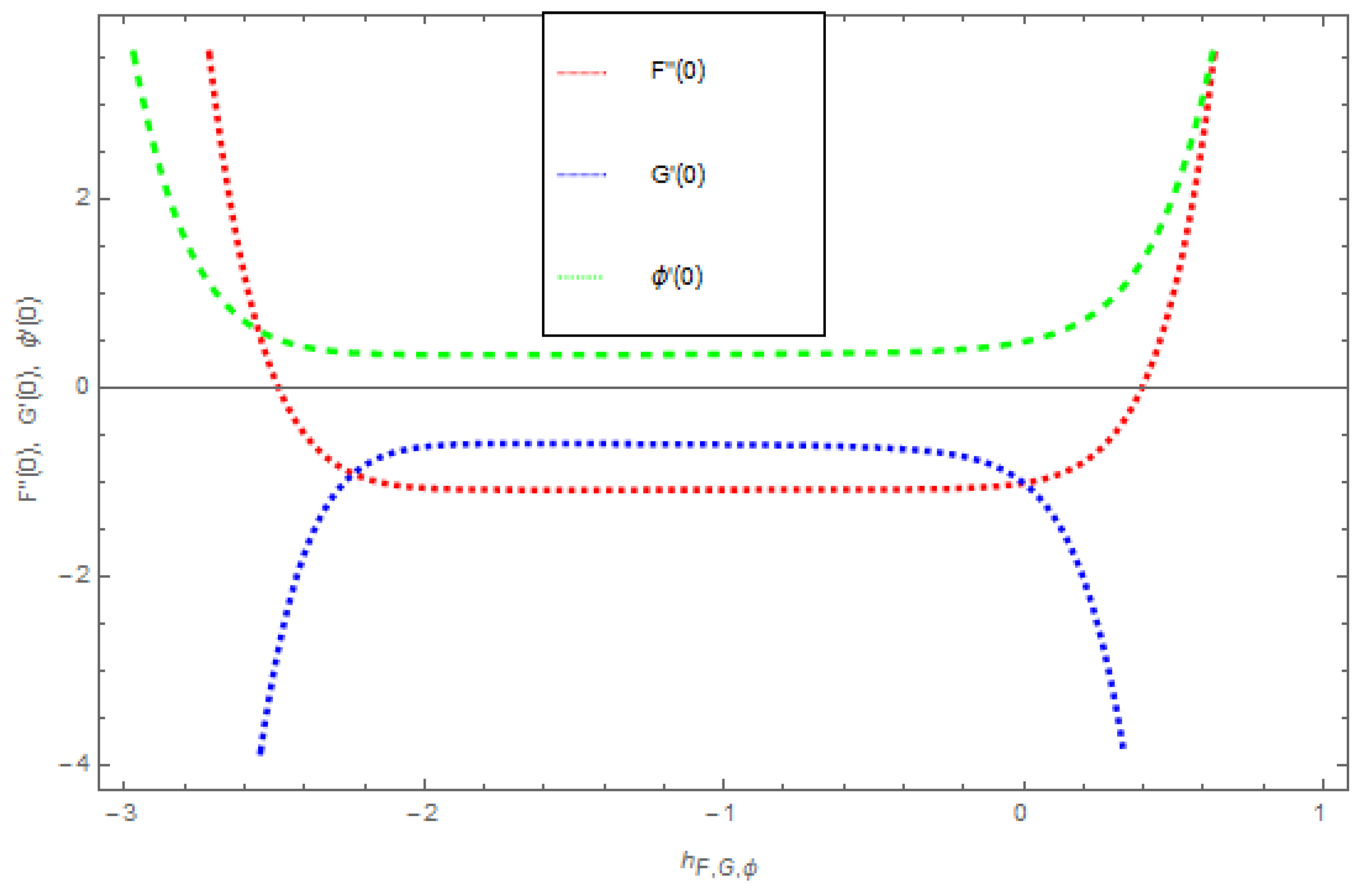
4. HAM Solution Convergences

In this segment we graphically discussed the superior effect of the concerned parameters. The convergence of Equation (36) was subjected entirely through the auxiliary constraints F , G , ϕ . This is a collection in a way that it controls and converges the series solutions. The optional division of , was plotted through -curves F ( 0 ) , G ( 0 ) , ϕ ( 0 ) for the 2 nd ordered approximated solution of HAM. The operational region of is 2.2 < F < 0.2 , 2.1 < G < 0.1 , 2.4 < ϕ < 0.1 . The convergence of HAM through the -curve on velocity profile F ( 0 ) , temperature profile G ( 0 ) and concentration profile ϕ ( 0 ) is presented in Figure 1.

5. Results and Discussion

In this segment the impact of emerging parameters on velocity function F ( η ) , temperature function G ( η ) and concentration function ϕ ( η ) within the defined domain have been discussed. The impact of M on F ( η ) is deliberated in Figure 2. The Lorentz force theory deliberated that the magnetic field grows at a reversed force to the fluids flow. This force reduced the momentum boundary layer while it improved the thickness of the boundary layer. Therefore, with the escalating magnetic field M the velocity profile F ( η ) declined. From here we concluded that Jeffrey nanofluid was greatly subjected by the magnetic field compared to the other two. In Figure 3 and Figure 4 the impact of Pr and Ω on G ( η ) were presented respectively. In Figure 3 we perceived that G ( η ) diminished with the rise in Pr . Physically the thickness of the boundary layer increased with the reduction in thermal diffusion. In addition, it can also be seen from the figure that Pr is more effective on Jeffrey and Maxwell nanofluids compared to the Oldroyd-B nanofluid. In Figure 4 the effect of thermal relaxation parameter Ω on G ( η ) has been described. From here we saw that G ( η ) reduced with the escalation in Ω . This was attributable to the fact that as we escalate Ω , the material particles need more time for heat transmission to its nearest particles. In addition, it can be stated that this material shows a non-conducting behavior with higher values of Ω which results in a reduction in G ( η ) . The impact of S c , K and K s on ϕ ( η ) are schemed in Figure 5, Figure 6 and Figure 7 respectively. In Figure 5 the effect of S c on ϕ ( η ) has been described. Schmidt number is the ratio of momentum diffusivity to mass diffusivity. Physically, the Schmidt number is related to hydrodynamic layer’s thickness and boundary layer. The escalating S c intensifies the momentum of the boundary layer flow which results in an increase in concentration profile. It is clear from the figure that ϕ ( η ) upsurges with the rise in S c . In Figure 6 the impact of K on ϕ ( η ) has been described. From here we concluded that larger K results in a reduction in ϕ ( η ) . This may have been caused by the fact that the reaction rates controlled the diffusion coefficients. To a certain extent similar results are displayed in Figure 7. In Figure 7 the impact of K s on ϕ ( η ) has been described. From this figure we have concluded that the growing values of K s showed a drop in behavior in ϕ ( η ) . This results from an agreement with the general physical behavior of the homogeneous reaction K and the heterogeneous reaction K s . In Figure 8 and Figure 9 the impact of M on C f x and N u x for Jeffrey, Maxwell and Oldroyd-B nanofluids have been described. It is clear from the figures that the growing values of M were decreasing for both C f x and N u x . The magnetic field was applied perpendicular to the flow of fluids and had an inverse variation with the skin friction of the fluid flow. This is the reason why the increasing magnetic field reduced the skin friction of the fluids flow. Similarly, the behavior of the heat transfer rate was due to the growing magnetic force on the fluids flow phenomena, with the fluid particles requiring more time to transfer the heat to the nearest particle. This was because the heat transfer rate reduced with the escalating magnetic field. The impact of Pr and Ω on N u x for the nanofluids flow has been described in Figure 10 and Figure 11. From here we have concluded that the escalation in Pr increased the heat transfer rate while the increased Ω reduced the heat transfer rate for the nanofluids flow. Figure 12 shows the Total Residual error for the three types of nanofluid flow.

Tables Discussion

In this section we have demonstrated the effect of emerging dimensionless parameters on the presented model of nanofluids. Table 1 displayed the conclusions associated with emerging parameters of skin fraction coefficients. This shows the impression of magenatic field parameter M on skin fraction coefficients. The magenatic field parameter shows a reduction in the skin fraction coefficient. Table 2 demonstrated the conclusion of incipient parameters on local Nusselt numbers. The heat transfer rate decreases with the rise in thermal relaxation parameter Ω while escalates with the increase in Prandtl number Pr. Table 2 shows that the thermal relaxation parameter has more effect on Jefferey nanofluids in comparison to Maxwell and Oldroyd-B nanofluids. Table 3 demonstrated the conclusion of an emerging parameter on the Sherwood number. The Sherwood number reduces with its rise, which upsurges with the escalation of the strength of homogeneous reaction K and the strength of heterogeneous reaction K s .

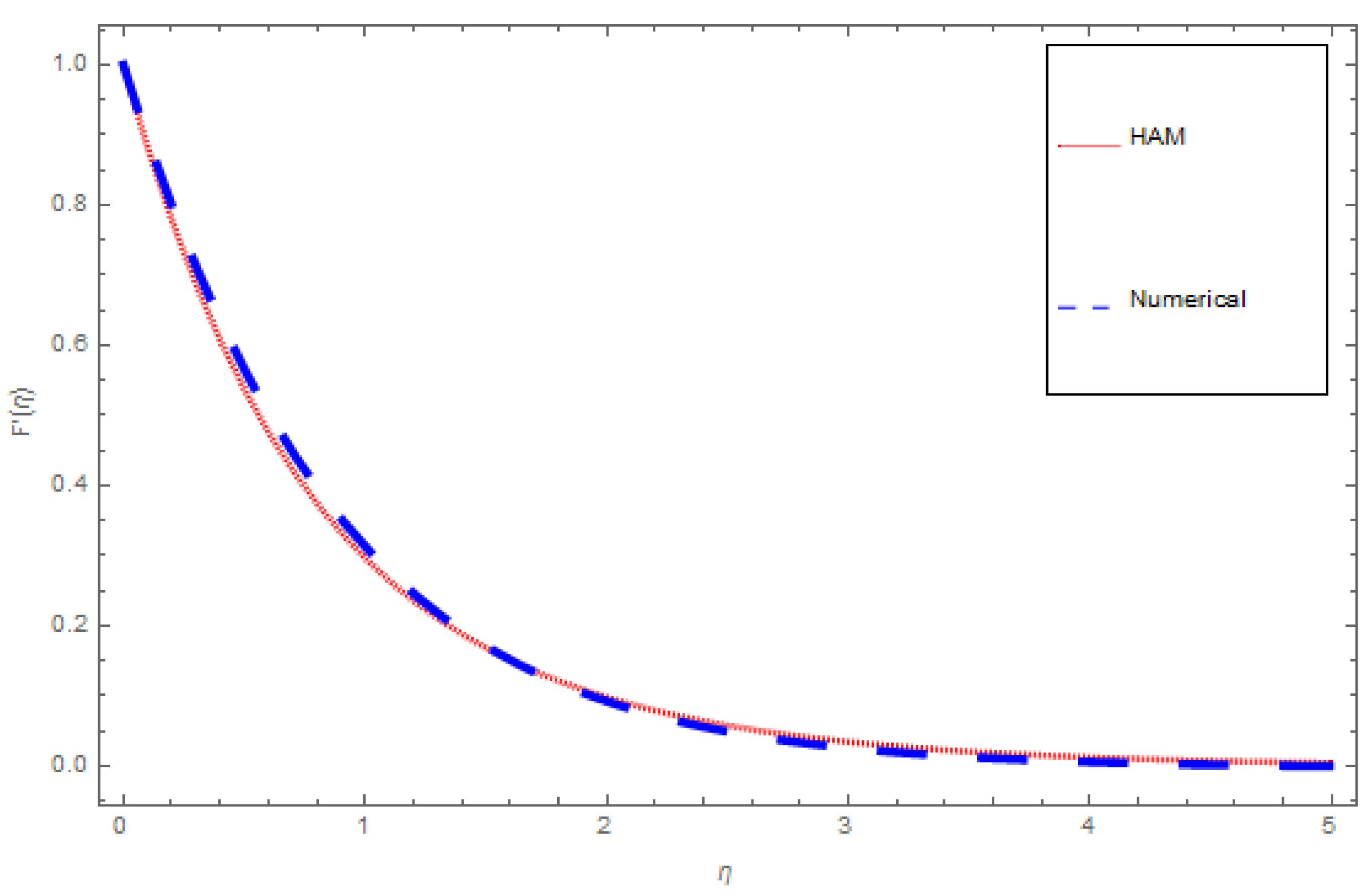
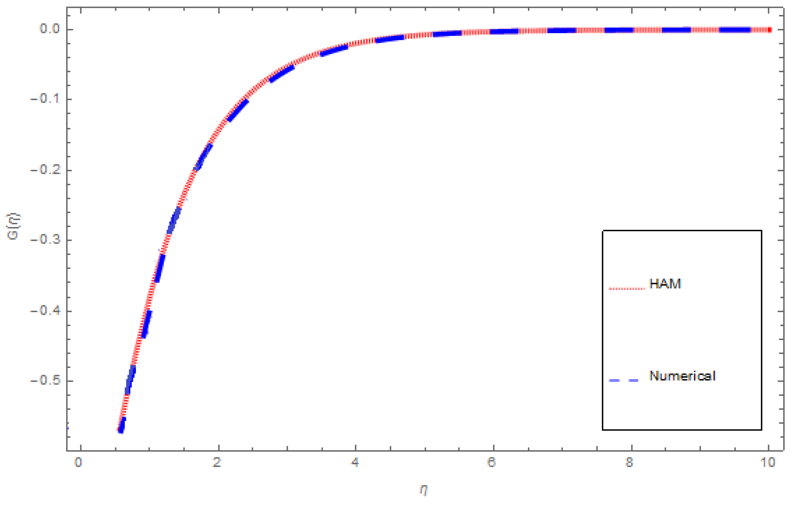
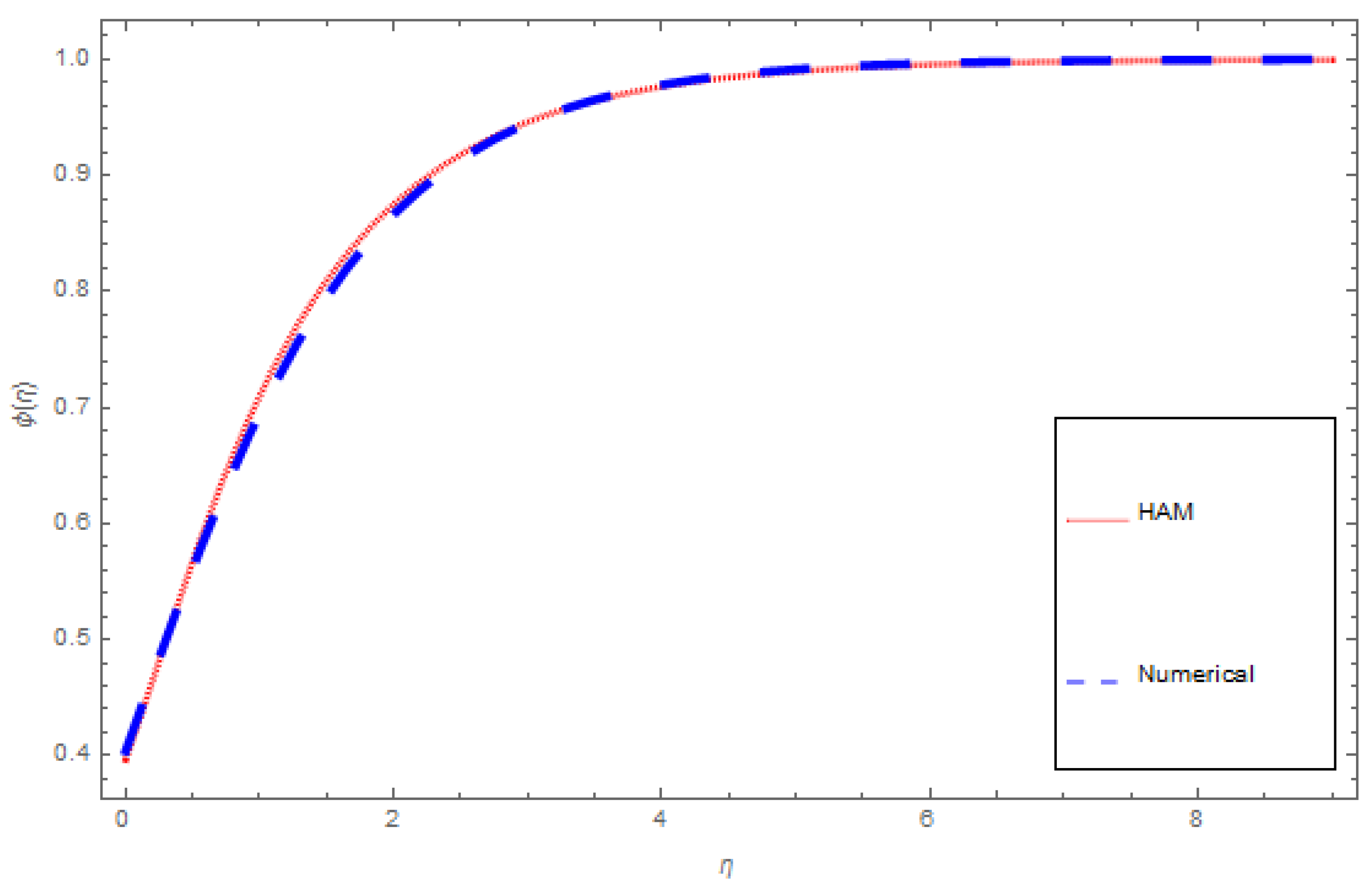
6. Comparison of Analytical Solutions and Numerical Solutions

An analytical solution means an exact solution. To study the behavior of systems, an analytical solution can be used with varying properties. Regrettably there are many practical systems that lead to an analytical solution, and analytical solutions are often of limited use. This is why we use a numerical approach to generate answers that are closer to practical results. These solutions which cannot be used as complete mathematical expressions are numerical solutions. In the natural worldthere are almost no problems that are exactly solvable, which makes the problem more difficult than all the exactly solvable problems. There are three or four of them in nature that have already been solved, unfortunately even numerical methods cannot always give an exact solution. Numerical techniques can handle any completed physical geometries which are often impossible to solve analytically. In this article both analytical and numerical approaches are tested to solve the modeled problem. A comparison of HAM and ND-Solve technique for F ( η ) , G ( η ) and ϕ ( η ) are deliberated in Figure 13, Figure 14 and Figure 15 and Table 4, Table 5 and Table 6, respectively.

7. Conclusions

In this article the MHD flow of three combined nanofluids (Jefferey, Maxwell, and Oldroyd-B) over a linear stretched surface have been scrutinized. The problem was solved analytically by HAM. The convergence of HAM has been presented through graphical presentations. The concluding remarks are as follows:
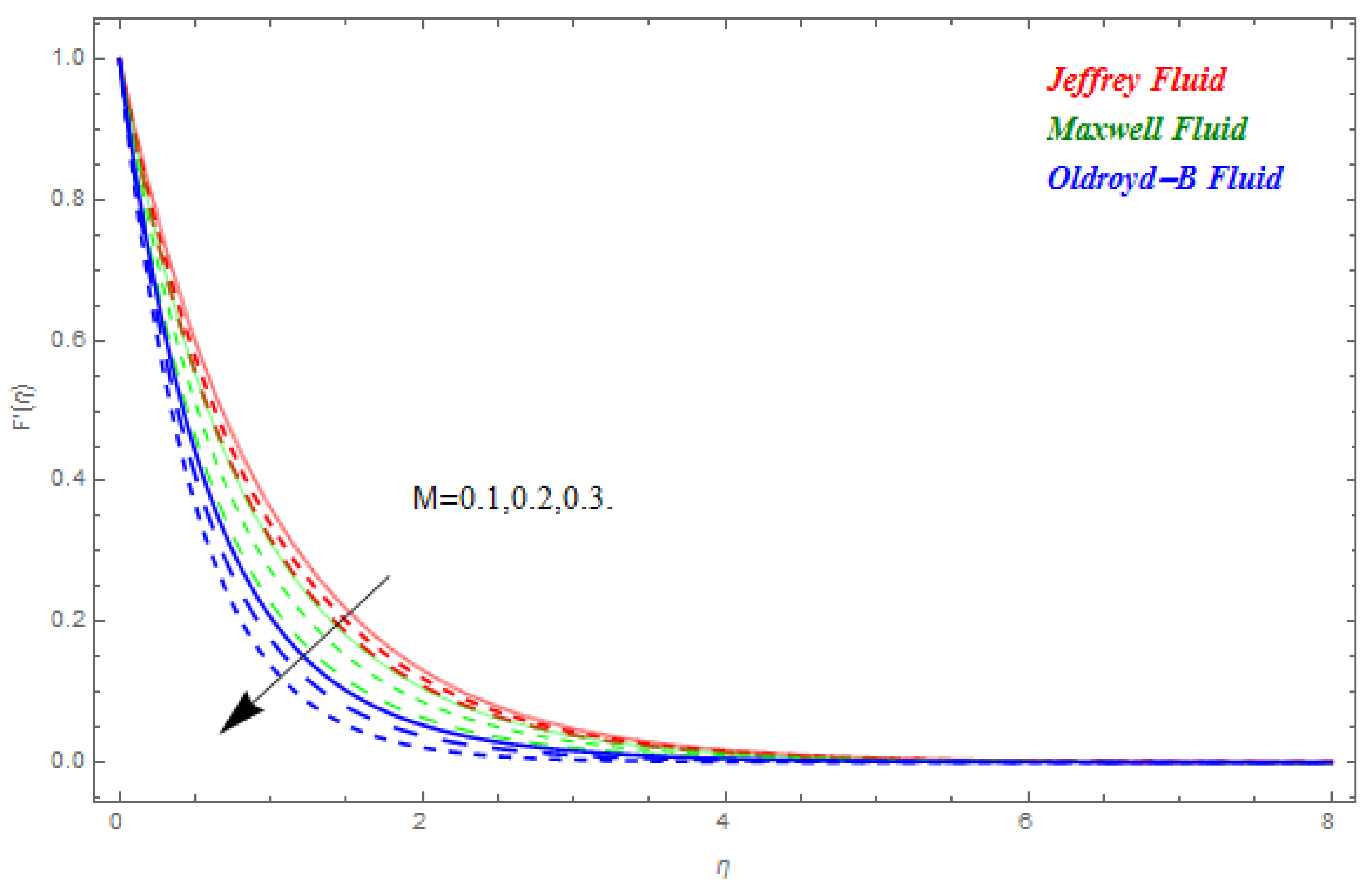
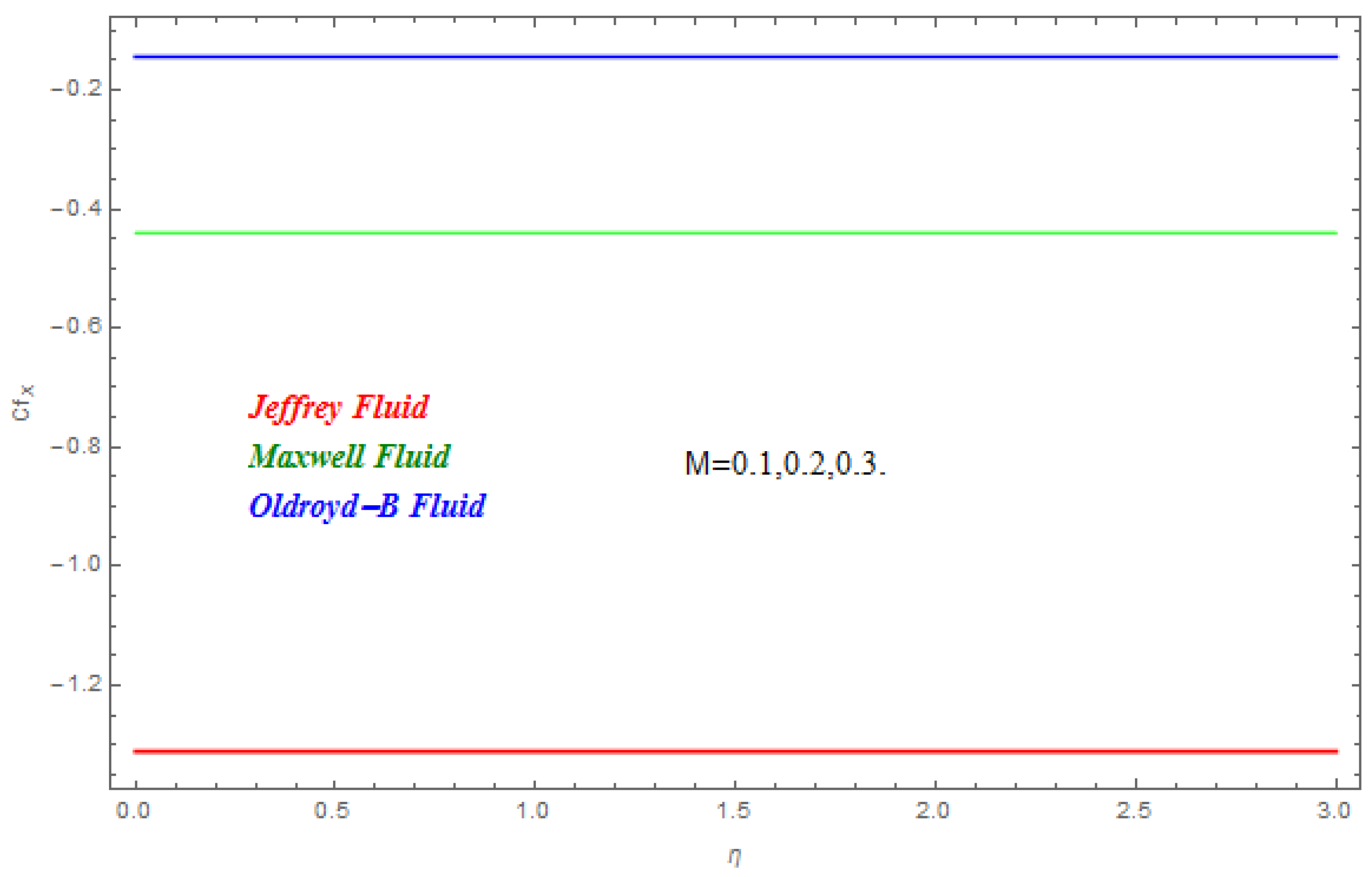
The upsurges in magnetic field diminishes the velocity field.
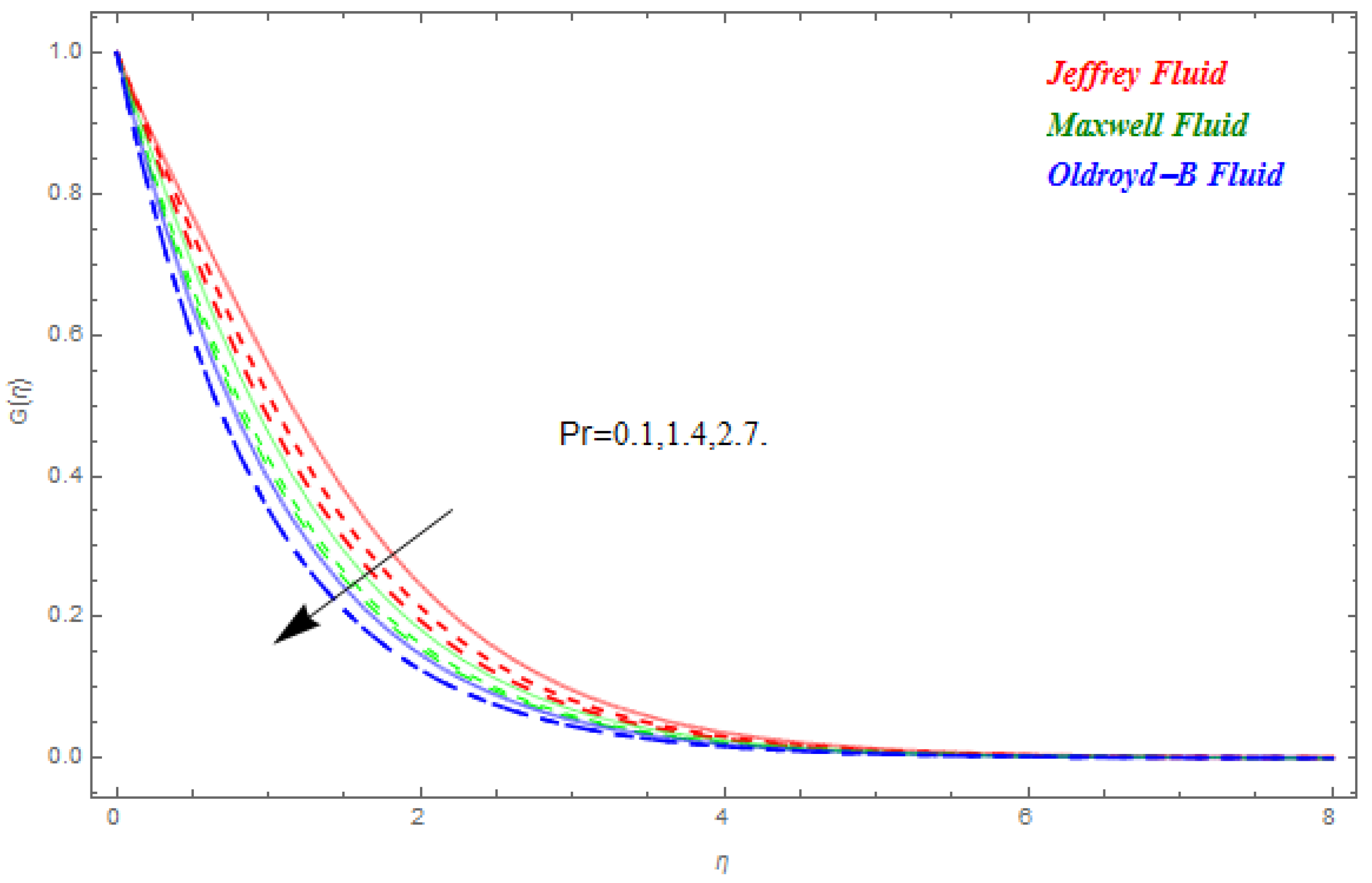
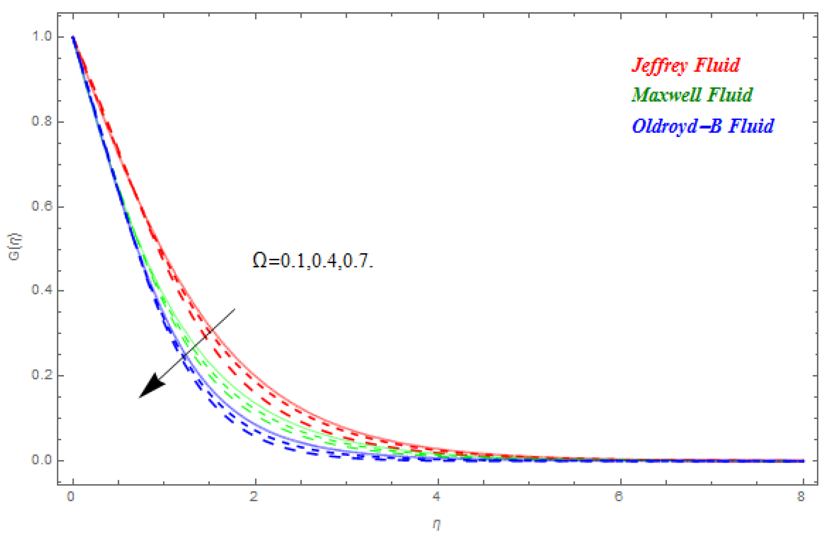
The upsurges in Prandtl number and thermal relaxation parameters diminish the temperature field.
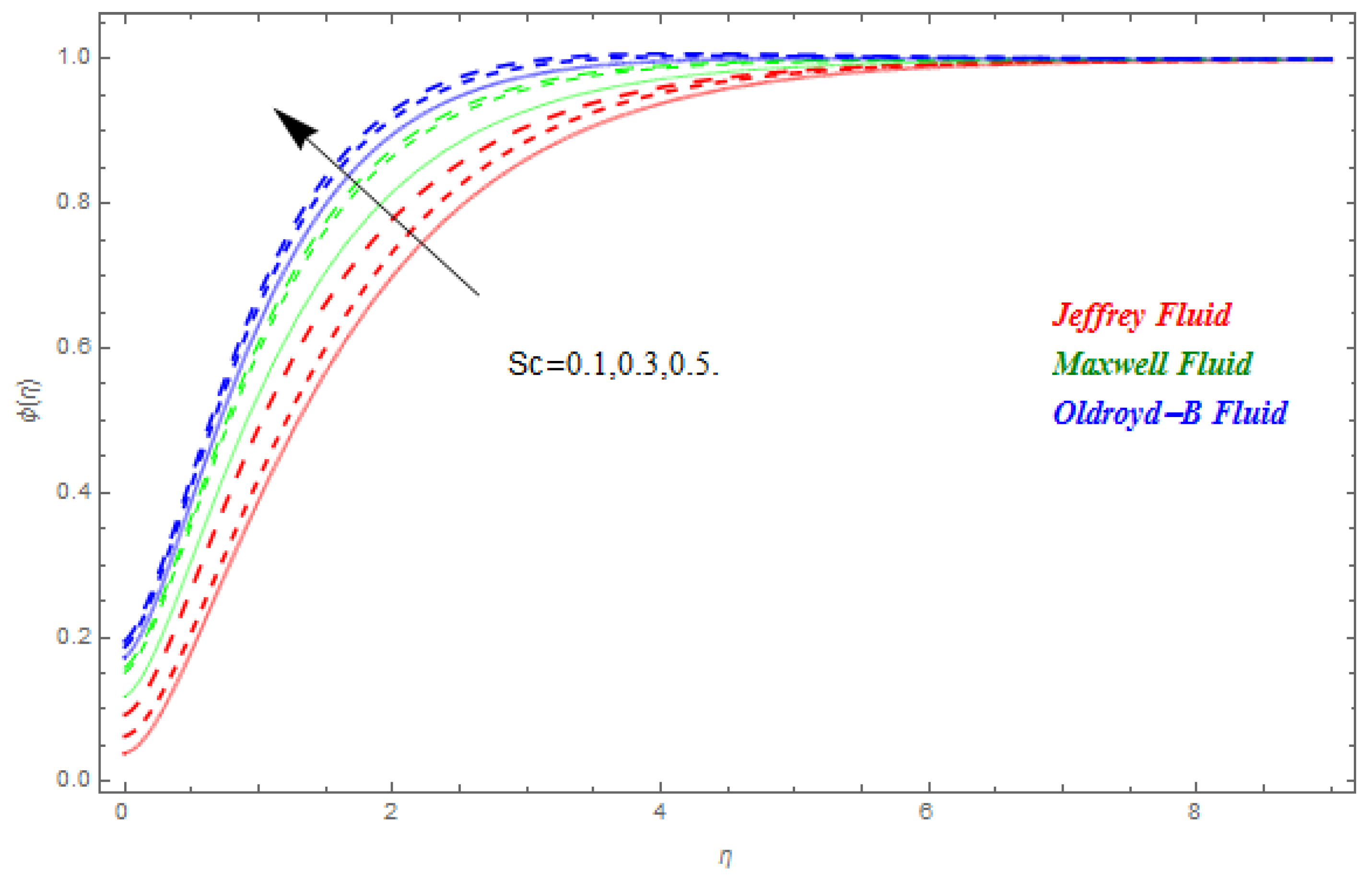
The upsurges in Schmidt number upsurges the concentration field.
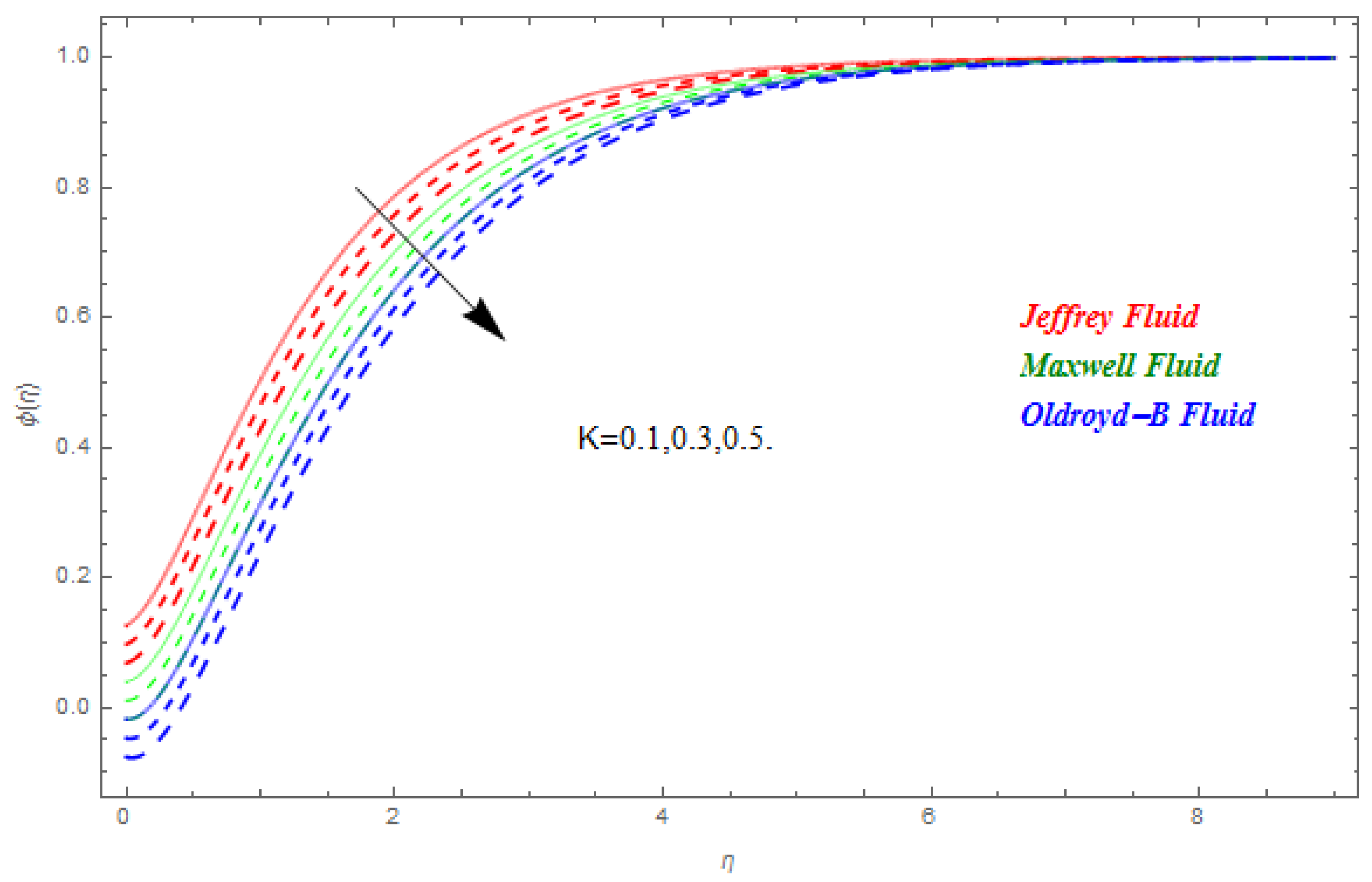
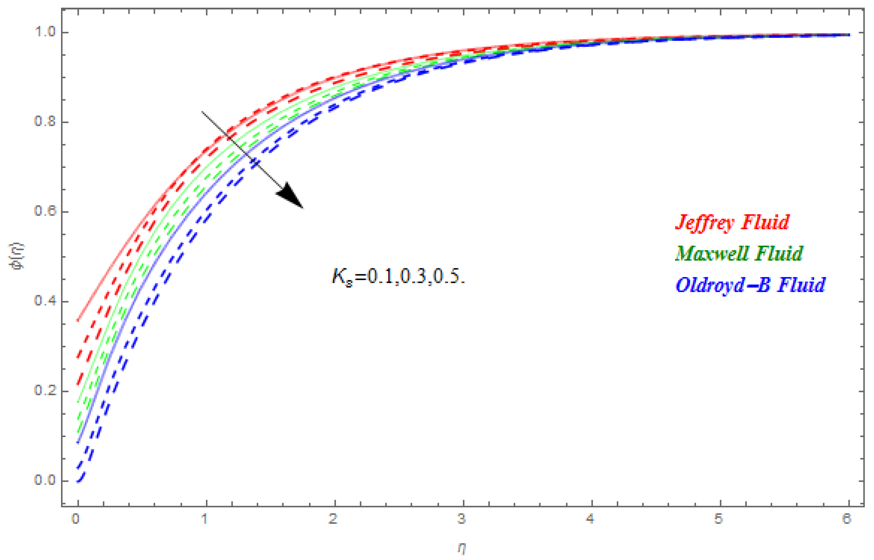
The larger homogeneous reaction and heterogeneous reaction strengths falloff from the concentration field.

Author Contributions

A.S. and Z.S. modeled the problem and wrote the manuscript. S.I., A.D. and P.K. thoroughly checked the mathematical modeling and English corrections. W.K. and A.S. solved the problem using Mathematica software. Z.S., S.I. and P.K. contributed to the results and discussions. All authors finalized the manuscript after its internal evaluation.

Conflicts of Interest

The authors declare no conflict of interest.

Nomenclature

B 0 Magnetic field strength (NmA−1)
C f x Skin friction coefficient
D I , D J Diffusion coefficients
F Velocity profile
G Temperature profile
I , J Chemical species
i, jConcentration
K Strength of homogenous reaction
K s Strength of heterogeneous reaction
k Thermal conductivity (Wm−1K−1)
M Magnetic parameter
N u x Nusselt number
Pr Prandtl number
q Heat flux (Wm−2)
Re x Local Reynolds number
S c Schmidt number
S h x Sherwood number
T Fluid temperature (K)
T w Surface temperature (K)
T Temperature at infinity (K)
u , v Velocity components (ms−1)
x , y Coordinates
α Thermal diffusivity (m2s−1)
η Similarity variable
μ Dynamic viscosity (mPa)
υ f Kinematic viscosity (mPa)
ρ f Density (Kgm−3)
λ 1 Relaxation time
λ 2 Relaxation to retardation time
λ 3 Retardation time
ζ Stretching rate
κ Deborah number
Ω Thermal relaxation parameter
σ Electrical conductivity (Sm−1)
ϕ Dimensional concentration profile

References

  1. Choi, S.U.S. Enhancing thermal conductivity of fluids with nanoparticles. Int. Mech. Eng. Congr. Expo. 1995, 66, 99–105. [Google Scholar]
  2. Fourier, J.B.J. TheÂorie Analytique De La Chaleur; Chez Firmin Didot, père et fils: Paris, France, 1822. [Google Scholar]
  3. Cattaneo, C. Sulla conduzione delcalore. Atti Semin Mat Fis Univ Modena Reggio Emilia 1948, 3, 83–101. [Google Scholar]
  4. Christov, C.I. On frame indifferent formulation of the Maxwell-Cattaneo model of finite-speed heat conduction. Mech. Res. Commun. 2009, 36, 481–486. [Google Scholar] [CrossRef]
  5. Mustafa, M. Cattaneo-Christov heat flux model for rotating flow and heat transfer of upper-convected Maxwell fluid. AIP Adv. 2015, 5, 047109. [Google Scholar] [CrossRef] [Green Version]
  6. Chen, C.H. Effect of viscous dissipation on heat transfer in a non-Newtonian liquid film over an unsteady stretching sheet. J. Non-Newton. Fluid Mech. 2005, 135, 128–135. [Google Scholar] [CrossRef]
  7. Sheikholeslami, M.; Shah, Z.; Shafi, A.; Khan, I.; Itili, I. Uniform magnetic force impact on water based nanofluid thermal behavior in a porous enclosure with ellipse shaped obstacle. Sci. Rep. 2019, 9, 1196. [Google Scholar] [CrossRef] [PubMed]
  8. Sheikholeslami, M.; Shah, Z.; Tassaddiq, A.; Shafee, A.; Khan, I. Application of Electric Field for Augmentation of Ferrofluid Heat Transfer in an Enclosure Including Double Moving Walls. IEEE Access 2019, 7, 21048–21056. [Google Scholar] [CrossRef]
  9. Sheikholeslami, M.; Haq, R.L.; Shafee, A.; Zhixiong, L. Heat transfer behavior of Nanoparticle enhanced PCM solidification through an enclosure with V shaped fins. Int. J. Heat Mass Transf. 2019, 130, 1322–1342. [Google Scholar] [CrossRef]
  10. Sheikholeslami, M.; Gerdroodbary, M.B.; Moradi, R.; Shafee, A.; Zhixiong, L. Application of Neural Network for estimation of heat transfer treatment of Al2O3-H2O nanofluid through a channel. Comput. Methods Appl. Mech. Eng. 2019, 344, 1–12. [Google Scholar] [CrossRef]
  11. Sheikholeslami, M. Numerical study of heat transfer enhancement in a pipe filled with porous media by axisymmetric TLB model based on GPU. Int. J. Heat Mass. Trans. 2014, 70, 1040–1049. [Google Scholar]
  12. Shah, Z.; Islam, S.; Gul, T.; Bonyah, E.; Altaf Khan, M. The Elcerical MHD And Hall Current Impact on Micropolar Nanofluid Flow Between Rotating Parallel Plates. Results Phys. 2018. [Google Scholar] [CrossRef]
  13. Shah, Z.; Bonyah, E.; Islam, S.; Gul, T. Impact of thermal radiation on electrical mhd rotating flow of carbon nanotubes over a stretching sheet. AIP Adv. 2019, 9, 015115. [Google Scholar] [CrossRef]
  14. Shah, Z.; Tassaddiq, A.; Islam, S.; Alklaibi, A.; Khan, I. Cattaneo–Christov Heat Flux Model for Three-Dimensional Rotating Flow of SWCNT and MWCNT Nanofluid with Darcy–Forchheimer Porous Medium Induced by a Linearly Stretchable Surface. Symmetry 2019, 11, 331. [Google Scholar] [CrossRef]
  15. Shah, Z.; Bonyah, E.; Islam, S.; Khan, W.; Ishaq., M. Radiative MHD thin film flow of Williamson fluid over an unsteady permeable stretching. Heliyon 2018, 4, e00825. [Google Scholar] [CrossRef] [PubMed]
  16. Dawar, A.; Shah, Z.; Khan, W.; Islam, S.; Idrees, M. An optimal analysis for Darcy-Forchheimer 3-D Williamson Nanofluid Flow over a stretching surface with convective conditions. Adv. Mech. Eng. 2019, 11, 1–15. [Google Scholar] [CrossRef]
  17. Shah, Z.; Islam, S.; Ayaz, H.; Khan, S. Radiative Heat and Mass Transfer Analysis of Micropolar Nanofluid Flow of Casson Fluid between Two Rotating Parallel Plates with Effects of Hall Current. ASME J. Heat Transf. 2019. [Google Scholar] [CrossRef]
  18. Maleki, H.; Safaei, M.R.; Alrashed, A.A.A.A.; Kasaeian, A. Flow and heat transfer in non-Newtonian nanofluids over porous surfaces. J. Anal. Calorim. 2019, 135, 1655. [Google Scholar] [CrossRef]
  19. Nasiri, H.; Abdollahzadeh Jamalabadi, M.Y.; Sadeghi, R.; Safaei, M.R.; Nguyen, T.K.; Shadloo, M.S. A smoothed particle hydrodynamics approach for numerical simulation of nano-fluid flows. J. Anal. Calorim. 2019, 135, 1733. [Google Scholar] [CrossRef]
  20. Rashidi, M.M.; Nasiri, M.; Shadloo, M.S.; Yang, Z. Entropy Generation in a Circular Tube Heat Exchanger Using Nanofluids: Effects of Different Modeling Approaches. Heat Transf. Eng. 2017, 38, 853–866. [Google Scholar] [CrossRef]
  21. Safaei, M.R.; Shadloo, M.S.; Goodarzi, M.S.; Hadjadj, A.; Goshayeshi, H.R.; Afrand, M.; Kazi, S.N. A survey on experimental and numerical studies of convection heat transfer of nanofluids inside closed conduits. Adv. Mech. Eng. 2016. [Google Scholar] [CrossRef]
  22. Mahian, O.; Kolsi, L.; Amani, M.; Estelle, P.; Ahmadi, G.; Kleinstreuer, C.; Marshall, J.S.; Siavashi, M.; Taylor, R.A.; Niazmand, H.; et al. Recent advances in modeling and simulation of nanofluid flows-Part I: Fundamentals and theory. Phys. Rep. 2019, 790, 1–48. [Google Scholar] [CrossRef]
  23. Mahian, O.; Kolsi, L.; Amani, M.; Estelle, P.; Ahmadi, G.; Kleinstreuer, C.; Marshall, J.S.; Taylor, R.A.; Abu-Nada, E.; Rashidi, S.; et al. Recent advances in modeling and simulation of nanofluid flows-Part II: Applications. Phys. Rep. 2019, 791, 1–59. [Google Scholar] [CrossRef]
  24. Kartini, A.; Zahir, H.; Anuar, I. Mixed convection Jeffrey fluid flow over an exponentially stretching sheet with magnetohydrodynamic effect. AIP Adv. 2016, 6, 035024. [Google Scholar] [Green Version]
  25. Kartini, A.; Anuar, I. Magnetohydrodynamic Jeffrey fluid over a stretching vertical surface in a porous medium. Propuls. Power Res. 2017, 6, 269–276. [Google Scholar]
  26. Hayat, T.; Hussain, T.; Shehzad, S.A.; Alsaedi, A. Flow of Oldroyd-B fluid with nano particles and thermal radiation. Appl. Math. Mech. Engl. Ed. 2015, 36, 69–80. [Google Scholar] [CrossRef]
  27. Raju, C.S.K.; Sandeep, N.; Gnaneswar, R.M. Effect of nonlinear thermal radiation on 3D Jeffrey fluid flow in the presence of homogeneous–heterogeneous reactions. Int. J. Eng. Res. Afr. 2016, 21, 52–68. [Google Scholar] [CrossRef]
  28. Raju, C.S.K.; Sandeep, N. Heat and mass transfer in MHD non-Newtonian bio-convection flow over a rotating cone/plate withcross diffusion. J. Mol. Liq. 2016, 215, 115–126. [Google Scholar] [CrossRef]
  29. Alla, A.M.A.; Dahab, S.M.A. Magnetic field and rotation effects on peristaltic transport on Jeffrey fluid in an asymmetric channel. J. Mag. Magn. Mater. 2015, 374, 680–689. [Google Scholar] [CrossRef]
  30. Khan, A.A.; Ellahi, R.; Usman, M. Effects of variable viscosity on the flow of non-Newtonian fluid through a porous medium in an inclined channel with slip conditions. J. Porous Media 2013, 16, 59–67. [Google Scholar] [CrossRef]
  31. Ellahi, R.; Bhatti, M.M.; Riaz, A.; Sheikholeslami, M. Effects of magnetohydrodynamics on peristaltic flow of Jeffrey fluid in a rectangular duct through a porous medium. J. Porous Media 2014, 17, 143–147. [Google Scholar] [CrossRef]
  32. Hayat, T.; Ali, N. A mathematical description of peristaltic hydromagnetic flow in a tube. Appl. Math. Comput. 2007, 188, 1491–1502. [Google Scholar] [CrossRef]
  33. Hayat, T.; Abbas, Z.; Sajid, M. Series solution for the upper convected Maxwell fluid over a porous stretching plate. Phys. Lett. A 2006, 358, 396–403. [Google Scholar] [CrossRef]
  34. Raju, C.S.K.; Sandeep, N. Heat and mass transfer in 3D non-Newtonian nano and Ferro fluids over a bidirectional stretching surface. Int. J. Eng. Res. Afr. 2016, 21, 33–51. [Google Scholar] [CrossRef]
  35. Sandeep, N.; Sulochana, C. Dual solutions for unsteady mixed convection flow of MHD micropolar fluid over a stretching/ shrinking sheet with non-uniform heat source/sink. Eng. Sci. Technol. Int. J. 2015, 18, 738–745. [Google Scholar] [CrossRef]
  36. Raju, C.S.K.; Sandeep, N.; Sulochana, C.; Sugunamma, V.; Jayachandra, B.M. Radiation, inclined magnetic field and cross diffusion effects on flow over a stretching surface. J. Niger. Math. Soc. 2015, 34, 169–180. [Google Scholar] [CrossRef]
  37. Nadeem, S.; Akbar, N.S. Influence of haet and mass transfer on a peristaltic motion of a Jeffrey-six constant fluid in an annulus. Heat Mass Transf. 2010, 46, 485–493. [Google Scholar] [CrossRef]
  38. Makinde, O.D.; Chinyoka, T.; Rundora, L. Unsteady flow of a reactive variable viscosity non-Newtonian fluid through a porous saturated medium with asymmetric convective boundary conditions. Comput. Math. Appl. 2011, 62, 3343–3352. [Google Scholar] [CrossRef] [Green Version]
  39. Sheikholeslami, M. KKL correlation for simulation of nanofluid flow and heat transfer in a permeable channel. Phys. Lett. A 2014, 378, 3331–3339. [Google Scholar] [CrossRef]
  40. Shah, Z.; Dawar, A.; Islam, S.; Khan, I.; Ching, D.L.C. Darcy-Forchheimer Flow of Radiative Carbon Nanotubes with Microstructure and Inertial Characteristics in the Rotating Frame. Case Stud. Therm. Eng. 2018, 12, 823–832. [Google Scholar] [CrossRef]
  41. Chai, L.R.; Shaukat, L.; Wang, H.; Wang, S. A review on heat transfer and hydrodynamic characteristics of nano/microencapsulated phase change slurry (N/MPCS) in mini/microchannel heat sinks. Appl. Therm. Eng. 2018. [Google Scholar] [CrossRef]
  42. Shah, Z.; Dawar, A.; Islam, S.; Khan, I.; Ching, D.L.C.; Khan, A.Z. Cattaneo-Christov model for Electrical Magnetite Micropoler Casson Ferrofluid over a stretching/shrinking sheet using effective thermal conductivity model. Case Stud. Therm. Eng. 2018. [Google Scholar] [CrossRef]
  43. Dawar, A.; Shah, Z.; Islam, S.; Idress, M.; Khan, W. Magnetohydrodynamic CNTs Casson Nanofluid and Radiative heat transfer in a Rotating Channels. J. Phys. Res. Appl. 2018, 1, 017–032. [Google Scholar]
  44. Khan, A.S.; Nie, Y.; Shah, Z.; Dawar, A.; Khan, W.; Islam, S. Three-Dimensional Nanofluid Flow with Heat and Mass Transfer Analysis over a Linear Stretching Surface with Convective Boundary Conditions. Appl. Sci. 2018, 8, 2244. [Google Scholar] [CrossRef]
  45. Imtiaz, M.; Hayat, T.; Alsaedi, A.; Hobiny, A. Homogeneous-heterogeneous reactions in MHD flow due to an unsteady curved stretching surface. J. Mol. Liq. 2016, 221, 245–253. [Google Scholar] [CrossRef]
  46. Hayat, T.; Hussain, Z.; Muhammad, T.; Alsaedi, A. Effects of homogeneous and heterogeneous reactions in flow of nanofluids over a nonlinear stretching surface with variable surface thickness. J. Mol. Liq. 2016, 221, 1121–1127. [Google Scholar] [CrossRef]
  47. Nasir, S.; Shah, Z.; Islam, S.; Khan, W.; Khan, S.N. Radiative flow of magneto hydrodynamics single-walled carbon nanotube over a convectively heated stretchable rotating disk with velocity slip effect. Adv. Mech. Eng. 2019, 11, 1–11. [Google Scholar]
  48. Nasir, S.; Shah, Z.; Islam, S.; Khan, W.; Bonyah, E.; Ayaz, M.; Khan, A. Three dimensional Darcy-Forchheimer radiated flow of single and multiwall carbon nanotubes over a rotating stretchable disk with convective heat generation and absorption. AIP Adv. 2019, 9, 035031. [Google Scholar] [CrossRef]
  49. Hammed, K.; Haneef, M.; Shah, Z.; Islam, I.; Khan, W.; Asif, S.M. The Combined Magneto hydrodynamic and electric field effect on an unsteady Maxwell nanofluid Flow over a Stretching Surface under the Influence of Variable Heat and Thermal Radiation. Appl. Sci. 2018, 8, 160. [Google Scholar] [CrossRef]
  50. Ullah, A.; Alzahrani, E.O.; Shah, Z.; Ayaz, M.; Islam, S. Nanofluids Thin Film Flow of Reiner-Philippoff Fluid over an Unstable Stretching Surface with Brownian Motion and Thermophoresis Effects. Coatings 2019, 9, 21. [Google Scholar] [CrossRef]
Figure 1. The combined -curves for F ( 0 ) , G ( 0 ) and   ϕ ( 0 ) .
Symmetry 11 00439 g001
Figure 2. Impact of M on F ( η ) , when Ω = 0.5 , S c = 0.6 , K = 0.8 , Pr = 0.7 , K s = 0.9 .
Symmetry 11 00439 g002
Figure 3. Impact of Pr on G ( η ) , when Ω = 0.5 , S c = 0.6 , K = 0.8 , M = 0.1 , K s = 0.9 .
Symmetry 11 00439 g003
Figure 4. Impact of Ω on G ( η ) , when S c = 0.6 , Pr = 0.7 , K = 0.8 , M = 0.1 , K s = 0.9 .
Symmetry 11 00439 g004
Figure 5. Impact of S c on ϕ ( η ) , when Ω = 0.1 , Pr = 0.7 , K = 0.8 , M = 0.1 , K s = 0.9 .
Symmetry 11 00439 g005
Figure 6. Impact of K on ϕ ( η ) , when Ω = 0.1 , Pr = 0.7 , S c = 0.6 , M = 0.1 , K s = 0.9 .
Symmetry 11 00439 g006
Figure 7. Impact of K s on ϕ ( η ) , when Pr = 0.7 , Ω = 0.1 , S c = 0.6 , M = 0.1 , K = 0.8 .
Symmetry 11 00439 g007
Figure 8. Impact of M on C f x .
Symmetry 11 00439 g008
Figure 9. Impact of M on N u x .
Symmetry 11 00439 g009
Figure 10. Impact of Pr on N u x .
Symmetry 11 00439 g010
Figure 11. Impact of Ω on N u x .
Symmetry 11 00439 g011
Figure 12. Total residual error for Jeffery, Maxwell and Oldroyd-B nanofluids.
Symmetry 11 00439 g012
Figure 13. HAM versus numerical comparison for F ( η ) .
Symmetry 11 00439 g013
Figure 14. HAM versus numerical comparison for G ( η ) .
Symmetry 11 00439 g014
Figure 15. HAM versus numerical comparison for ϕ ( η ) .
Symmetry 11 00439 g015
Table 1. Distinction in C f x for different M .
MRef. [47]Present Results for Jeffrey NanofluidRef. [47]Present Results for Maxwell NanofluidRef. [47]Present Results for Oldroyd-B Nanofluid
1.01.2104580.2104621.5041511.5041531.0710191.071022
2.01.4315841.4315871.8047881.8047911.2480811.248084
Table 2. Distinction in N u x for different Ω and Pr .
ΩPrRef. [47]Jeffrey NanofluidRef. [47]Maxwell NanofluidRef. [47]Oldroyd-B Nanofluid
1.0----------0.610394----------0.595298----------0.610846
1.2----------0.607503----------0.593311----------0.607993
6.00.4180810.5137860.4211670.5112470.4264760.5154367
7.00.4396950.6268650.4419190.5489660.4476700.5477974
Table 3. Distinction in S h x for different S c , K and K s .
ScKKsJeffreyMaxwellOldroyd-B
1.2−0.096477−0.095593−0.096771
1.5−0.096782−0.095890−0.097081
1.5−0.058030−0.047238−0.049135
1.7−0.056699−0.037230−0.039262
0.5−0.018933−0.0372330.012399
0.8−0.1600280.046603−0.125205
Table 4. Symmetry of HAM versus numerical solutions for F ( η ) , when S c = Pr = K 2 = 1.0 , κ = κ 1 = κ 2 = λ 2 = M = K = 0.1 .
η HAM
F ( η )
Numerical
F ( η )
Absolute Error
AE
0.03.33067 × 10160.0000003.33067 × 1016
0.10.09504330.0933340.002876
0.20.1808270.1739720.009647
0.30.2582600.2427910.016488
0.40.3281650.3005780.020276
0.50.3912810.3480330.019089
0.60.4482770.3857770.011828
0.70.4997530.4143570.085396
0.80.5462510.4342620.111989
0.90.5882580.4459230.142335
1.00.6262130.4497300.176483
Table 5. Symmetry of HAM versus numerical solutions for G ( η ) , when S c = Pr = K s = 1.0 , κ = κ 1 = κ 2 = λ 3 = M = K = 0.1 .
η HAM
G ( η )
Numerical
G ( η )
Absolute Error
AE
0.01.0000001.000000.000000
0.10.9151650.8874770.002876
0.20.8357250.7759170.009647
0.30.7618450.6661950.016488
0.40.6935060.5590770.020276
0.50.6305630.455220.019089
0.60.5727910.3551650.011828
0.70.5199120.2593420.250570
0.80.4716180.1680730.303545
0.90.4275940.08158110.346013
1.00.3875185.60459 × 10−90.387517
Table 6. Symmetry of HAM versus numerical solutions for ϕ ( η ) , when S c = Pr = K s = 1.0 , κ = κ 1 = κ 2 = λ 2 = M = K = 0.1 .
η HAM
ϕ ( η )
Numerical
ϕ ( η )
Absolute Error
AE
0.00.3967620.4040800.007318
0.10.4298840.4364250.006841
0.20.4646670.4686060.003939
0.30.4998300.5003490.000519
0.40.5344900.5314180.003072
0.50.5680560.5616180.006438
0.60.6001460.5907890.009357
0.70.6305330.6188100.011723
0.80.6591020.6455890.013513
0.90.6858110.6710650.014746
1.00.7106750.6952020.015473

