A New Ranking Methodology for Pythagorean Trapezoidal Uncertain Linguistic Fuzzy Sets Based on Einstein Operations

Abstract

In this article, we proposed new Pythagorean trapezoidal uncertain linguistic fuzzy aggregation information—namely, the Pythagorean trapezoidal uncertain linguistic fuzzy Einstein weighted averaging (PTULFEWA) operator, the Pythagorean trapezoidal uncertain linguistic fuzzy Einstein ordered weighted averaging (PTULFEOWA) operator, and the Pythagorean trapezoidal uncertain linguistic fuzzy Einstein hybrid weighted averaging (PTULFEHWA) operator—using the Einstein operational laws. We studied some important properties of the suggested aggregation operators and showed that the PTULFEHWA is more general than the other proposed operators, which simplifies these aggregation operators. Furthermore, we presented a multiple attribute group decision making (MADM) process for the proposed aggregation operators under the Pythagorean trapezoidal uncertain linguistic fuzzy (PTULF) environment. A numerical example was constructed to determine the effectiveness and practicality of the proposed approach. Lastly, a comparative analysis was performed of the presented approach with existing approaches to show that the proposed method is consistent and provides more information that may be useful for complex problems in the decision-making process.

1. Introduction

The communication of the decision-making process is a very complex problem when we are receiving information about attributes. One the most powerful theories is that of the multi attribute decision making (MADM), which handles problems that extensively impact the human real-life problems. The basic methodology is that a decision maker is presented with his evaluation in a set of many attributes and alternatives to find the best ranking order alternative in MADM approaches. Zadeh [1] introduced a fuzzy set with the generalization of a classical set to solve ambiguous and vague information. Fuzzy set is used in many practical situations and has grown as an independent theory that interests researchers in many fields. After the success, fuzzy set was generalized to intuitionistic fuzzy set (IFS) by Atanassov [2] under the restriction that the membership and non-membership function sum was less than or equal to one. In [2] proposed a different mathematical operation under the IFS environment and studied the important properties. Uncertainty in human real problems is one of the continuous research areas and produces many new theories. Fuzzy decision-making (FDM) problems and their extension are presented in different ways to solve real life problems and have more attractive research to obtain the best results. Many decision making (DM) techniques have been proposed to explain the multi attribute decision-making process. Ramon et al. [3] presented the 2-tuple model and customer segmentation and their algorithms, k-means, which are more effective methods in the calculation of frequency and monetary exploitation.

Revanasiddappa and Harish [4] presented a new feature selection technique based on intuitionistic fuzzy entropy (IFE) for text classification. Firstly, intuitionistic fuzzy C-means (IFCM) clustering technique is employed to compute the intuitionistic membership values. The computed intuitionistic membership values are then used to estimate intuitionistic fuzzy entropy via match degree. Additionally, features with lower entropy values are selected to categorize the text documents. Juan Antonio Morente-Molinera et al. [5] focused on solving the problem by carrying out multi-criteria group decision making approaches using different new methods. Concretely, fuzzy ontologies reasoning procedures are used in order to reduce, at the very least, the experts needed to participate in the preference providing step. In this new advanced technique, the logic of alternative comparison relies on the ontology reasoning process, allowing experts to focus on how important the criteria are to them. Albadan et al. [6] proposed the procedures of selection of personnel delimited only to the making of non-programmed decisions through the implementation of game mechanics. In order to model this selection, the purpose of the following study is to carry out the formulation of inference rules based on fuzzy logic in order to capture the tacit transfer of certain types of information in personnel selection processes and to determine the aspects that allow the shaping of aspirants. In [7], the author defined generalized operation for intuitionistic fuzzy numbers.

Morente-Molinera proposed the technique of fuzzy ontologies in order to allow the experts to focus on determining the importance that should be given to different criteria. Thus, they deal directly with a high number of alternatives. Experts decide the importance of each criterion, and the alternatives ranking is calculated automatically using the fuzzy ontology. Liang et al. [8] presented the partial estimations, which determined that the introduced estimator is more capable and trusted to evaluate, consequently improving the overall results. There are many methodologies that evaluate the overall information that converges in different suppositions. If an ordinary collection of information is not considered in this environment, there is other information that can be considered by linguistic variables (LV) related to FNs, which are related to the membership function to one and the non-membership function to zero—more precisely, “good” and “bad”. Wang et al. [9] proposed ILS, and their MADM approach of using the IL aggregation information achieved some great consideration. Liu et al. [10] presented a new power aggregation operator, while Su et al. [11] generalized the concept to ordered weighted averaging (OWA) and intuitionistic linguistic ordered weighted averaging (ILOWA) operator. Xiao et al. [12] studied the ILOWA operator and applied it in the financial DM process. Liu and Jin [13] extended the intuitionistic uncertain linguistic values (IULVs) by using LV in intuitionistic linguistic variables (ILV) and studying their important properties. We observed that LVs are special facets of IULVs, which are more general and have more information. Liu et al. [14] presented and extended the linguistic (LF) aggregation operators. Yager [15] introduced a new Pythagorean fuzzy (PFS) set that is a generalization of IFS by membership and non-membership functions under the condition that the square sum of these functions is less than or equal to one. To motivate this idea, Yager [16] explained this shortcoming with an example—a decision maker makes a decision in the form of MD as $\left(\frac{\sqrt{3}}{2}\right)$, a N-MD is $\frac{1}{2}$. Under IFS, the value does not satisfy the condition of a sum greater than 1, while in PFS, it satisfies the condition that the square sum is less than or equal to 1. After the successful implementation, Peng and Yang [17] presented the different aggregation operators, namely, the Pythagorean fuzzy weighted averaging (PFWA), the Pythagorean fuzzy weighted power averaging (PFWPA), and the Pythagorean fuzzy weighted power geometric (PFWPG) operator. Garg [18] introduced a new generalized Pythagorean fuzzy aggregation operator using Einstein operational laws and used them in the decision- making process.

Shakeel et al. [19] presented some aggregation operators to use the decision information represented by PTFNS, including the Pythagorean trapezoidal fuzzy weighted averaging (PTFWA) operator, the Pythagorean trapezoidal fuzzy ordered weighted averaging (PTFOWA) operator, and the Pythagorean trapezoidal fuzzy hybrid averaging (PTFHA) operator. Shakeel et al. [20] extended the work of aggregation operators into the interval-valued Pythagorean trapezoidal fuzzy weighted averaging (IVPTFWA) operator, the ordered weighted (IVPTFOWA), and the hybrid averaging (IVPTFHA) operators. Shakeel et al. [20] used Einstein operational laws and proposed a new concept of the Pythagorean trapezoidal fuzzy Einstein ordered weighted geometric (I-IVPTFEOWG) operator, the induced interval-valued Pythagorean trapezoidal fuzzy Einstein hybrid geometric (I-IVPTFEHG) operator, and their applications in decision making problems. Shakeel et al. [21] further extended the work to interval-valued Pythagorean trapezoidal fuzzy aggregation operators, the interval-valued Pythagorean trapezoidal fuzzy Einstein weighted geometric, (IVPTFEWG) operator, the interval-valued Pythagorean trapezoidal fuzzy Einstein ordered weighted geometric (IVPTFEOWG) operator, the interval-valued Pythagorean trapezoidal fuzzy Einstein hybrid geometric (IVPTFEHG), and their applications in decision making. The detail literature survey of aggregation operators and their applications in decision making problems discussed in [22,23,24,25,26,27,28,29,30,31,32].

In this paper, we introduce a new aggregation operator using Einstein operations under trapezoidal uncertain linguistic fuzzy sets and their applications in decision making. The motivations for the study are listed below.

(1)

Our anticipated aggregation information is more general and precise compared to the existing information.

(2)

The objectives of the study include proposing a PTULF Einstein aggregation operator and its operational laws, score, and accuracy function, establishing the MADM program approach based on the PTULF Einstein aggregation operators, and providing illustrative examples of the MADM program.

(3)

The comparative analysis is a strong testament to the new approach, as it shows that the proposed study is consistent.

To solve a MADM process, the weight of the attributes plays an important role in making decisions under the aggregation approaches.

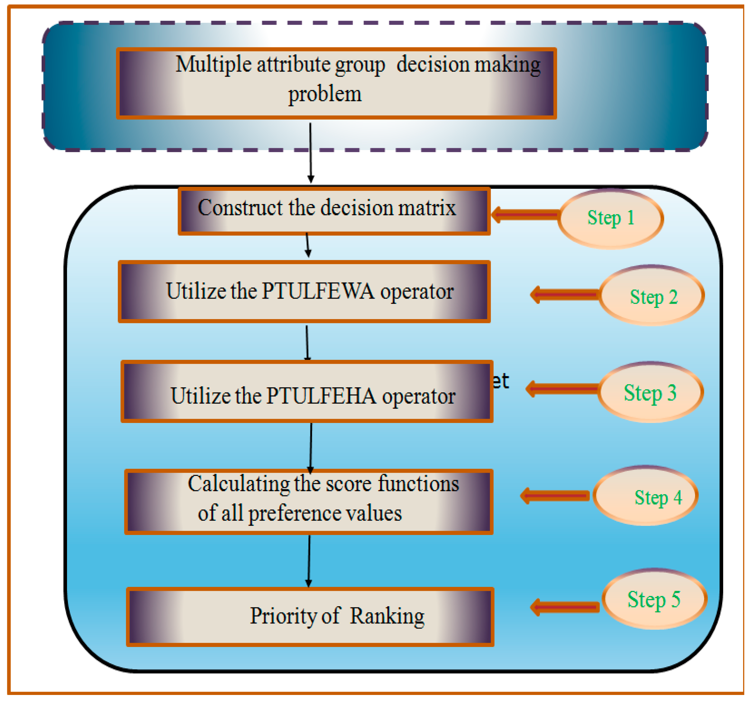
The rest of the paper is arranged is follows. Section 2 consists of the background materials. Section 3 presents a new PTULF aggregation operator under Einstein operations, the Pythagorean trapezoidal uncertain linguistic fuzzy Einstein weighted averaging (PTULFEWA) operator, the Pythagorean trapezoidal uncertain linguistic fuzzy Einstein ordered weighted averaging (PTULFEOWA), and the Pythagorean trapezoidal uncertain linguistic fuzzy Einstein hybrid averaging (PTULFEHA) operator. Section 4 describes the MADM technique under the PTFL environment. In Section 5, a numerical example is given to demonstrate the importance of the methodologies. Section 6 shows a comparative study of the proposed and existing approaches. The conclusion is given in Section 7.

2. Preliminaries

Definition 1.

[10]. Let $[s_{\theta \left(p\right)},s_{t\left(p\right)}]\in \overline{s}$, and $P$ is a given domain as follows:

$$U=\{[s_{\theta \left(p\right)},s_{t\left(p\right)}],({\mathrm{\Psi }}_u(p),{\mathsf{\Upsilon }}_u(p))]:p\in P\},$$

(1)

is called an intuitionistic uncertain linguistic set (IULS), where $s_{\theta \left(p\right)},s_{t\left(p\right)}\in \overline{s}$. Where ${\mathrm{\Psi }}_u(p)$ and ${\mathsf{\Upsilon }}_u(p)$ represent the MD and N-MD, respectively, with the condition $0\le {\mathrm{\Psi }}_u(p)+{\mathsf{\Upsilon }}_u(p)\le 1,$ $\forall p\in P$. The MD and N-MD of the element $p$ to the ULV $[s_{\theta \left(p\right)},s_{t\left(p\right)}].$ For each $ILS,$ $U$ in $p,$ if ${\pi }_U(p)=1-{\mathrm{\Psi }}_U(p)-{\mathsf{\Upsilon }}_U(p),$ for all $p\in P,$ then ${\pi }_u(p)$ is called the degree of indeterminacy degree of $p$ to the ULV $[s_{\theta \left(p\right)},s_{t\left(p\right)}].$ It is obvious that $0\le {\pi }_u(p)\le 1,$ $\forall p\in P.$

Definition 2.

[10]. Let $U=\{[s_{\theta \left(p\right)},s_{t\left(p\right)}],({\mathrm{\Psi }}_u(p),{\mathsf{\Upsilon }}_u(p))]\}:p\in P\},$ be (IULS), the quaternion $\langle [s_{\theta \left(p\right)},s_{t\left(p\right)}],({\gamma }_u(p),{\mathsf{\varsigma }}_u(p))]\rangle$ is called an $IULV,$ and $U$ can also be viewed as a collection of the $IULV$. Thus, it can also be expressed as follows:

$$U=\{[s_{\theta \left(p\right)},s_{t\left(p\right)}],({\mathrm{\Psi }}_u(p),{\mathsf{\Upsilon }}_u(p))]\}:p\in P\}.$$

(2)

Definition 3.

[24] Let ${\tilde{\alpha }}_1=(\left[p_1,q_1,r_1,s_1\right];{\mathrm{\Psi }}_{{\tilde{\alpha }}_1},{\mathsf{\Upsilon }}_{{\tilde{\alpha }}_1}),$ and ${\tilde{\alpha }}_2=(\left[p_2,q_2,r_2,s_2\right];{\mathrm{\Psi }}_{{\tilde{\alpha }}_2},{\mathsf{\Upsilon }}_{{\tilde{\alpha }}_2})$ be two ITF numbers and $\delta \ge 0.$ Then,

(1) 

${\tilde{\alpha }}_1\oplus {\tilde{\alpha }}_2=\left(\begin{array}{c}\left[p_1+p_2,q_1+q_2,r_1+r_2,s_1+s_2\right];\\ ({\mathrm{\Psi }}_{{\tilde{\alpha }}_1})+({\mathrm{\Psi }}_{{\tilde{\alpha }}_2})-({\mathrm{\Psi }}_{{\tilde{\alpha }}_1}{\mathrm{\Psi }}_{{\tilde{\alpha }}_2}),{\mathsf{\Upsilon }}_{{\tilde{\alpha }}_1}{\mathsf{\Upsilon }}_{{\tilde{\alpha }}_2}\end{array}\right)$

(2) 

${\tilde{\alpha }}_1\otimes {\tilde{\alpha }}_2=\left(\begin{array}{c}\left[p_1{p}_2,q_1{q}_2,r_1{r}_2,s_1{s}_2\right];\\ {\mathrm{\Psi }}_{{\tilde{\alpha }}_1}{\mathrm{\Psi }}_{{\tilde{\alpha }}_2},({\mathsf{\Upsilon }}_{{\tilde{\alpha }}_1})+({\mathsf{\Upsilon }}_{{\tilde{\alpha }}_2})-({\mathsf{\Upsilon }}_{{\tilde{\alpha }}_1}{\mathsf{\Upsilon }}_{{\tilde{\alpha }}_2})\end{array}\right)$

(3) 

$\delta \tilde{\alpha }=(\left[\delta p,\delta q,\delta r,\delta s\right];1-{\left(1-{\mathrm{\Psi }}_{\tilde{\alpha }}\right)}^{\delta };{({\mathsf{\Upsilon }}_{\tilde{\alpha }})}^{\delta })$

(4) 

${\tilde{\alpha }}^{\delta }=(\left[p^{\delta },q^{\delta },r^{\delta },s^{\delta }\right];{\mathrm{\Psi }}_{\tilde{\alpha }}^{\delta },1-{\left(1-{\mathsf{\Upsilon }}_{\tilde{\alpha }}\right)}^{\delta }).$

Example 1.

Let $=\left(\left[0.2,0.3,0.4,0.5\right];\left(0.5,0.3\right)\right)$ ${\alpha }_1=\left(\left[0.1,0.3,0.3,0.2\right];\left(0.3,0.6\right)\right)$, ${\alpha }_2=\left(\left[0.8,0.2,0.6,0.1\right];\left(0.4,0.2\right)\right)$ be any three ITFNs, and $\delta =0.2.$ Then, we verify the above results such that,

(1) 

${\tilde{\alpha }}_1\oplus {\tilde{\alpha }}_2=\left(\begin{array}{c}[0.9,0.5,0.9,0.3];\\ (0.3)+(0.4)-\left(0.3\right)\left(0.4\right),\left(0.6\right)\left(0.2\right)\end{array}\right)=\left([0.9,0.5,0.9,0.3];0.58,0.12\right).$

(2) 

${\tilde{\alpha }}_1\otimes {\tilde{\alpha }}_2=\left(\begin{array}{c}[0.08,0.06,0.18,0.02];\\ \left(0.3\right)\left(0.4\right),\left(0.6\right)+\left(0.2\right)-\left(0.6\right)\left(0.2\right)\end{array}\right)=([0.08,0.06,0.18,0.02];(0.12,0.68).$

(3) 

$\delta \tilde{\alpha }=\left(\begin{array}{c}[0.2(0.2),0.2(0.3),0.2(0.4),0.2(0.5)];\\ 1-{\left(1-0.5\right)}^{0.2},{\left(0.3\right)}^{0.2}\end{array}\right)=[0.04,0.06,0.08,0.1];(0.25,0.78).$

(4) 

${\tilde{\alpha }}^{\delta }=\left(\begin{array}{c}[{(0.2)}^{0.2},{(0.3)}^{0.2},{(0.4)}^{0.2},{(0.5)}^{0.2}];\\ {\left(0.5\right)}^{0.2},1-{\left(1-0.3\right)}^{0.2}\end{array}\right)=\left(\begin{array}{c}[(0.72),(0.78),(0.83),(0.87)];\\ \left(0.87\right),0.06\end{array}\right).$

Definition 4.

[15]. Let $L$ be a fixed set. The $PFS,$ $U$ in $L$ is an object having the form;

$$A=\left\{\langle l,{\mathrm{\Psi }}_U(l),{\mathsf{\Upsilon }}_U(l)\rangle \right|l\in L\}$$

(3)

Definition 5.

[16]. Let $\tilde{\alpha }=\left({\mathrm{\Psi }}_{\tilde{\alpha }},{\mathsf{\Upsilon }}_{\tilde{\alpha }}\right),$ ${\tilde{\alpha }}_1=\left({\mathrm{\Psi }}_{{\tilde{\alpha }}_1},{\mathsf{\Upsilon }}_{{\tilde{\alpha }}_1}\right)$ and ${\tilde{\alpha }}_2=\left({\mathrm{\Psi }}_{{\tilde{\alpha }}_2},{\mathsf{\Upsilon }}_{{\tilde{\alpha }}_2}\right)$ be three $PFNs$ and $\delta >0.$ Then,

(1) 

${\tilde{\alpha }}^c=\left({\mathsf{\Upsilon }}_{\tilde{\alpha }},{\mathrm{\Psi }}_{\tilde{\alpha }}\right)$

(2) 

${\tilde{\alpha }}_1\oplus {\tilde{\alpha }}_2=\left(\sqrt{{({\mathrm{\Psi }}_{{\tilde{\alpha }}_1})}^2+{({\mathrm{\Psi }}_{{\tilde{\alpha }}_2})}^2-({\mathrm{\Psi }}_{{\tilde{\alpha }}_1}^2{\mathrm{\Psi }}_{{\tilde{\alpha }}_2}^2)},{\mathsf{\Upsilon }}_{{\tilde{\alpha }}_1}{\mathsf{\Upsilon }}_{{\tilde{\alpha }}_2}\right)$

(3) 

${\tilde{\alpha }}_1\otimes {\tilde{\alpha }}_2=\left({\mathrm{\Psi }}_{{\tilde{\alpha }}_1}{\mathrm{\Psi }}_{{\tilde{\alpha }}_2},\sqrt{{({\mathsf{\Upsilon }}_{{\tilde{\alpha }}_1})}^2+{({\mathsf{\Upsilon }}_{{\tilde{\alpha }}_2})}^2-({\mathsf{\Upsilon }}_{{\tilde{\alpha }}_1}^2{\mathsf{\Upsilon }}_{{\tilde{\alpha }}_2}^2)}\right)$

(4) 

$\delta \tilde{\alpha }=\sqrt{1-{\left(1-{\mathrm{\Psi }}_{\tilde{\alpha }}^2\right)}^{\delta }};{({\mathsf{\Upsilon }}_{\tilde{\alpha }})}^{\delta })$

(5) 

${\tilde{\alpha }}^{\delta }=({\mathrm{\Psi }}_{\tilde{\alpha }}^{\delta },\sqrt{1-{\left(1-{\mathsf{\Upsilon }}_{\tilde{\alpha }}^2\right)}^{\delta }}).$

Example 2.

Let $\tilde{\alpha }=(0.8,0.3),$ ${\tilde{\alpha }}_1=(0.5,0.6)$, ${\tilde{\alpha }}_2=(0.4,0.7)$ be any three PFNs, and $\delta =0.3.$ Then, we verify the above results such that,

(1) 

${\tilde{\alpha }}_1\oplus {\tilde{\alpha }}_2=\left(\begin{array}{c}\sqrt{{(0.5)}^2+{(0.4)}^2-({0.5}^2)({0.4}^2)},\\ \left(0.6\right)\left(0.7\right)\end{array}\right)=\left(\sqrt{0.37},0.42\right)=(0.85,0.17).$

(2) 

${\tilde{\alpha }}_1\otimes {\tilde{\alpha }}_2=\left(\begin{array}{c}\left(0.5\right)\left(0.4\right),\\ \sqrt{{(0.6)}^2+{(0.7)}^2-{(0.6)}^2({0.7}^2)}\end{array}\right)=\left(\left(0.5\right)\left(0.4\right),\sqrt{0.6736}\right)=(0.20,0.82).$

(3) 

$\delta \tilde{\alpha }=(\sqrt{1-{\left(1-{0.8}^2\right)}^{0.3}};{(0.3)}^{0.3})=(0.50,0.69).$

(4) 

${\tilde{\alpha }}^{\delta }=({(0.8)}^{0.3},\sqrt{1-{\left(1-{0.3}^2\right)}^{0.3}})=(0.93,0.16).$

Definition 6.

[19] Let $\tilde{\alpha }=(\left[p,q,r,s\right];[{\mathrm{\Psi }}_{\tilde{\alpha }},{\mathsf{\Upsilon }}_{\tilde{\alpha }}])$ be a PTFN, the score function $s$ is;

$$s(\tilde{\alpha })=\left(\frac{p+q+r+s}{4}\cdot \left({\mathrm{\Psi }}_{\tilde{\alpha }}^2-{\mathsf{\Upsilon }}_{\tilde{\alpha }}^2\right)\right)s(\tilde{\alpha })\in [-1,1].$$

(4)

Example 3.

Let ${\tilde{p}}_1=\left\{\left[0.4,0.3,0.5,0.6\right];\left(0.6,0.5\right)\right\}$, ${\tilde{p}}_2=\left\{\left[0.1,0.4,0.3,0.2\right];\left(0.7,0.4\right)\right\}$ and ${\tilde{p}}_3=\left\{\left[0.2,0.1,0.6,0.5\right];\left(0.8,0.5\right)\right\}$ be PTFNs, a score new example function $S$ of PTFNs can be represented as follows:

$$\begin{array}{l}S({\tilde{p}}_1)=\frac{0.4+0.3+0.5+0.6}{4}({0.6}^2-{0.5}^2)=0.0495,\\ S({\tilde{p}}_2)=\frac{0.1+0.4+0.3+0.2}{4}({0.7}^2-{0.4}^2)=0.060,\\ S({\tilde{p}}_3)=\frac{0.2+0.1+0.6+0.5}{4}({0.8}^2-{0.5}^2)=0.1365.\end{array}$$

Definition 7.

[19]. Let $\tilde{\alpha }=(\left[p,q,r,s\right];[\mathrm{\Psi },\mathsf{\Upsilon }])$ be PTFN, an accuracy function $h$ is:

$$h(\tilde{\alpha })=\left(\frac{p+q+r+s}{4}\cdot \left({\mathrm{\Psi }}_{\tilde{\alpha }}^2+{\mathsf{\Upsilon }}_{\tilde{\alpha }}^2\right)\right)h(\tilde{\alpha })\in [0,1].$$

(5)

Example 4.

Let ${\tilde{p}}_1=\left\{\left[0.4,0.3,0.5,0.6\right];\left(0.6,0.5\right)\right\}$, ${\tilde{p}}_2=\left\{\left[0.1,0.4,0.3,0.2\right];\left(0.7,0.4\right)\right\}$ and ${\tilde{p}}_3=\left\{\left[0.2,0.1,0.6,0.5\right];\left(0.8,0.5\right)\right\}$ be PTFNs, an accuracy new example function $h$ of PTFNs can be represented as follows:

$$\begin{array}{l}h({\tilde{p}}_1)=\frac{0.4+0.3+0.5+0.6}{4}({0.6}^2+{0.5}^2)=0.2745,\\ S({\tilde{p}}_2)=\frac{0.1+0.4+0.3+0.2}{4}({0.7}^2+{0.4}^2)=0.1625,\\ S({\tilde{p}}_3)=\frac{0.2+0.1+0.6+0.5}{4}({0.8}^2+{0.5}^2)=0.3115.\end{array}$$

Einstein Operations with Pythagorean Trapezoidal Fuzzy Numbers

The main Einstein operational laws are defined as follows:

$$a{\otimes }_{\epsilon }b=\frac{a.b}{\sqrt{1+\left(1-a^2\right)\cdot \left(1-b^2\right)}},a{\otimes }_{\epsilon }b=\frac{\sqrt{\left(a^2+b^2\right)}}{\sqrt{\left(1+a^2\cdot b^2\right)}},\mathrm{for}\mathrm{all}\left(a,b\right)\in {\left[0,1\right]}^2$$

(6)

Definition 8.

[20]. Let $\tilde{\alpha }=\left\{\begin{array}{c}\left[p,q,r,s\right];\\ ({\mathrm{\Psi }}_{\tilde{\alpha }},{\mathsf{\Upsilon }}_{\tilde{\alpha }})\end{array}\right\}$, ${\tilde{\alpha }}_1=\left\{\begin{array}{c}\left[p_1,q_1,r_1,s_1\right];\\ ({\mathrm{\Psi }}_{{\tilde{\alpha }}_1},{\mathsf{\Upsilon }}_{{\tilde{\alpha }}_1})\end{array}\right\}$ and ${\tilde{\alpha }}_2=\left\{\begin{array}{c}\left[p_2,q_2,r_2,s_2\right];\\ ({\mathrm{\Psi }}_{{\tilde{\alpha }}_2},{\mathsf{\Upsilon }}_{{\tilde{\alpha }}_2})\end{array}\right\}$ be any three $PTF$, numbers and $\delta \ge 0.$ Then,

(1) 

${\tilde{\alpha }}_1\oplus {\tilde{\alpha }}_2=\left\{\begin{array}{l}\left[p_1+p_2,q_1+q_2,r_1+r_2,s_1+s_2\right];\\ \sqrt{{({\mathrm{\Psi }}_{{\tilde{\alpha }}_1})}^2+{({\mathrm{\Psi }}_{{\tilde{\alpha }}_2})}^2-{({\mathrm{\Psi }}_{{\tilde{\alpha }}_1}{\mathrm{\Psi }}_{{\tilde{\alpha }}_2})}^2},{\mathsf{\Upsilon }}_{{\tilde{\alpha }}_1}{\mathsf{\Upsilon }}_{{\tilde{\alpha }}_2}\end{array}\right\}$

(2) 

${\tilde{\alpha }}_1\otimes {\tilde{\alpha }}_2=\left\{\begin{array}{c}\left[p_1{p}_2,q_1{q}_2,r_1{r}_2,s_1{s}_2\right];{\mathrm{\Psi }}_{{\tilde{\alpha }}_1}{\mathrm{\Psi }}_{{\tilde{\alpha }}_2},\\ \sqrt{{({\mathsf{\Upsilon }}_{{\tilde{\alpha }}_1})}^2+{({\mathsf{\Upsilon }}_{{\tilde{\alpha }}_2})}^2-{({\mathsf{\Upsilon }}_{{\tilde{\alpha }}_1}{\mathsf{\Upsilon }}_{{\tilde{\alpha }}_2})}^2}\end{array}\right\}$

(3) 

$\delta \tilde{\alpha }=\left\{(\left[\delta p,\delta q,\delta r,\delta s\right];\sqrt{1-{\left(1-{\mathrm{\Psi }}_{\tilde{\alpha }}^2\right)}^{\delta }};{({\mathsf{\Upsilon }}_{\tilde{\alpha }})}^{\delta })\right\}$

(4) 

${\tilde{\alpha }}^{\delta }=\left\{(\left[p^{\delta },q^{\delta },r^{\delta },s^{\delta }\right];{\mathrm{\Psi }}_{\tilde{\alpha }}^{\delta },\sqrt{1-{\left(1-{\mathsf{\Upsilon }}_{\tilde{\alpha }}^2\right)}^{\delta }})\right\}.$

Example 5.

Let $\tilde{\alpha }=\left\{\begin{array}{c}\left(s_2,s_3\right)\\ \left[0.3,0.4,0.5,0.6\right]\\ \left(0.7,0.4\right)\end{array}\right\},{\tilde{\alpha }}_1=\left\{\begin{array}{c}\left(s_3,s_6\right)\\ \left[0.3,0.4,0.5,0.6\right]\\ \left(0.8,0.5\right)\end{array}\right\}$ and ${\tilde{\alpha }}_2=\left\{\begin{array}{c}\left(s_4,s_3\right)\\ \left[0.5,0.3,0.4,0.4\right]\\ \left(0.8,0.3\right)\end{array}\right\}$ be any three $PTULFNS$ and $\delta =0.4.$ Then, we verify the results as follows:

(1) 

$\begin{array}{cc}\hfill {\tilde{\alpha }}_1\oplus {\tilde{\alpha }}_2& =\left(\begin{array}{c}[0.3+0.5,0.4+0.3,0.5+0.4,0.6+0.4];\\ \sqrt{{(0.8)}^2+{(0.8)}^2-{(0.8)}^2{(0.8)}^2},(0.5)(0.3)\end{array}\right)=\left(\begin{array}{c}[0.8,0.7,0.9,0.6+1.0];\\ \sqrt{(0.64)+(0.64)-(0.64)(0.64},(0.5)(0.3)\end{array}\right)\hfill \\ & =\left([0.8,0.7,0.9,0.6+1.0];\left(0.93,0.15\right)\right)\hfill \end{array}$

(2) 

$\begin{array}{cc}\hfill {\tilde{\alpha }}_1\otimes {\tilde{\alpha }}_2& =\left(\begin{array}{c}[\left(0.8\right)\left(0.5\right),\left(0.4\right)\left(0.3\right),\left(0.5\right)\left(0.4\right),\left(0.6\right)\left(0.4\right);\\ \left(0.8\right)\left(0.8\right),\sqrt{{0.5}^2+{0.3}^2-({\left(0.5\right)}^2{(0.3)}^2},\end{array}\right)=\left(\begin{array}{c}[0.4,0.12,0.20,0.24];\\ (0.64),\sqrt{0.25+0.09-0.0225},\end{array}\right)\hfill \\ & =\left([0.4,0.12,0.20,0.24;(0.64,0.5634\right)\hfill \end{array}$

(3) 

$\begin{array}{cc}\hfill \delta \tilde{\alpha }& =\left(\begin{array}{c}\left[\left(0.4\right)\left(0.3\right),\left(0.4\right)\left(0.4\right),\left(0.4\right)\left(0.5\right),\left(0.4\right)\left(0.6\right)\right];\\ \left[\sqrt{1-{\left(1-{0.7}^2\right)}^{0.4}},{(0.4)}^{0.4}\right],\end{array}\right)=\left(\begin{array}{c}\left[0.12,0.16,0.20,0.16\right];\\ \sqrt{1-{\left(1-{0.7}^2\right)}^{0.4}},{(0.4)}^{0.4},\end{array}\right)\hfill \\ & =\left(\begin{array}{c}\left[0.12,0.16,0.20,0.16\right];\\ \left(0.4859,0.6901\right)\end{array}\right)\hfill \end{array}$

(4) 

$\begin{array}{cc}\hfill {\tilde{\alpha }}^{\delta }& =\left(\begin{array}{c}\left[{0.3}^{0.4},{0.4}^{0.4},{0.5}^{0.4},{0.6}^{0.4}\right];,\\ \left[{0.4}^{0.4},\sqrt{1-{\left(1-{0.7}^2\right)}^{0.4}}\right]\end{array}\right)=\left(\begin{array}{c}\left[0.61,0.69,0.75,0.85\right];,\\ \left[{0.4}^{0.4},\sqrt{1-{\left(1-{0.7}^2\right)}^{0.4}}\right]\end{array}\right)\hfill \\ & =\left(\left[0.61,0.69,0.75,0.85\right];,(0.69,0.48)\right).\hfill \end{array}$

Definition 9.

Consider $\tilde{\alpha }=\left\{\begin{array}{c}\left(s_{\theta \left(p\right)},s_{t\left(p\right)}\right)\\ \left[p,q,r,s\right]\\ \left({\mathsf{\Psi }}_{\alpha },{\mathsf{{\rm Y}}}_{\alpha }\right)\end{array}\right\},{\tilde{\alpha }}_1=\left\{\begin{array}{c}\left(s_{\theta \left(p\right)},s_{t\left(p\right)}\right)\\ \left[p_1,q_1,r_1,s_1\right]\\ \left({\mathsf{\Psi }}_{{\alpha }_1},{\mathsf{{\rm Y}}}_{{\alpha }_1}\right)\end{array}\right\}$ and ${\tilde{\alpha }}_2=\left\{\begin{array}{c}\left(s_{\theta \left(p_2\right)},s_{t\left(p_2\right)}\right)\\ \left[p_2,q_2,r_2,s_2\right]\\ \left({\mathsf{\Psi }}_{{\alpha }_2},{\mathsf{{\rm Y}}}_{{\alpha }_2}\right)\end{array}\right\}$ be a PTULNs and $\delta \ge 0.$ Then

(1) 

${\tilde{\alpha }}_1{\oplus }_{\epsilon }{\tilde{\alpha }}_2=\left\{\begin{array}{c}(s_{\theta \left(p_1\right)}+s_{\theta \left(p_2\right)},s_{t\left(p_1\right)}+s_{t\left(p_2\right)}),\\ \left[p_1+p_2,q_1+q_2,r_1+r_2,s_1+s_2\right];\\ \frac{\sqrt{{({\mathrm{\Psi }}_{{\tilde{\alpha }}_1})}^2+{({\mathrm{\Psi }}_{{\tilde{\alpha }}_2})}^2}}{\sqrt{1+{({\mathrm{\Psi }}_{{\tilde{\alpha }}_1})}^2{({\mathrm{\Psi }}_{{\tilde{\alpha }}_2})}^2}},\frac{{\mathsf{\Upsilon }}_{{\tilde{\alpha }}_1}{\mathsf{\Upsilon }}_{{\tilde{\alpha }}_2}}{\sqrt{1+(1-{\mathsf{\Upsilon }}_{{\tilde{\alpha }}_1}^2)(1-{\mathsf{\Upsilon }}_{{\tilde{\alpha }}_2}^2)}}\end{array}\right\}$

(2) 

${\tilde{\alpha }}_1{\otimes }_{\epsilon }{\tilde{\alpha }}_2=\left\{\begin{array}{c}(s_{\theta \left(p_1\right)}{s}_{\theta \left(p_2\right)},s_{t\left(p_1\right)}{s}_{t\left(p_2\right)}),\\ \left[p_1{p}_2,q_1{q}_2,r_1{r}_2,s_1{s}_2\right];\\ \frac{{\mathrm{\Psi }}_{{\tilde{\alpha }}_1}{\mathrm{\Psi }}_{{\tilde{\alpha }}_2}}{\sqrt{1+(1-{\mathrm{\Psi }}_{{\tilde{\alpha }}_1}^2)(1-{\mathrm{\Psi }}_{{\tilde{\alpha }}_2}^2)}},\frac{\sqrt{{({\mathsf{\Upsilon }}_{{\tilde{\alpha }}_1})}^2+{({\mathsf{\Upsilon }}_{{\tilde{\alpha }}_2})}^2}}{\sqrt{1+{({\mathsf{\Upsilon }}_{{\tilde{\alpha }}_1})}^2{({\mathsf{\Upsilon }}_{{\tilde{\alpha }}_2})}^2}},\end{array}\right\}$

(3) 

${\delta }_{\stackrel{.}{\epsilon }}\tilde{\alpha }=\left\{\begin{array}{c}(s_{\delta \theta \left(p\right)},s_{\delta t\left(p\right)})\left[\delta p,\delta q,\delta r,\delta s\right];\\ \frac{\sqrt{{(1+{\mathrm{\Psi }}_{\tilde{\alpha }}^2)}^{\delta }-{(1-{\mathrm{\Psi }}_{\tilde{\alpha }}^2)}^{\delta }}}{\sqrt{{(1+{\mathrm{\Psi }}_{\tilde{\alpha }}^2)}^{\delta }+{(1-{\mathrm{\Psi }}_{\tilde{\alpha }}^2)}^{\delta }}},\frac{\sqrt{2{\left({\mathsf{\Upsilon }}_{\tilde{\alpha }}^2\right)}^{\delta }}}{\sqrt{{(2-{\mathsf{\Upsilon }}_{\tilde{\alpha }}^2)}^{\delta }+{({\mathsf{\Upsilon }}_{\tilde{\alpha }}^2)}^{\delta }}},\end{array}\right\}$

(4) 

${\tilde{\alpha }}^{{\wedge }_{\epsilon }\delta }=\left\{\begin{array}{c}(s_{\theta {\left(p\right)}^{\delta }},s_{t{\left(p\right)}^{\delta }}),\left[p^{\delta },q^{\delta },r^{\delta },s^{\delta }\right];\\ \frac{\sqrt{2{\left({\mathrm{\Psi }}_{\tilde{\alpha }}^2\right)}^{\delta }}}{\sqrt{{(2-{\mathrm{\Psi }}_{\tilde{\alpha }})}^{\delta }+{({\mathrm{\Psi }}_{\tilde{\alpha }})}^{\delta }}},\frac{\sqrt{{(1+{\mathsf{\Upsilon }}_{\tilde{\alpha }}^2)}^{\delta }-{(1-{\mathsf{\Upsilon }}_{\tilde{\alpha }}^2)}^{\delta }}}{\sqrt{{(1+{\mathsf{\Upsilon }}_{\tilde{\alpha }}^2)}^{\delta }+{(1-{\mathsf{\Upsilon }}_{\tilde{\alpha }}^2)}^{\delta }}}\end{array}\right\}.$

Example 6.

Let $\tilde{\alpha }=\left\{\begin{array}{c}\left(s_2,s_3\right)\\ \left[0.3,0.4,0.5,0.6\right]\\ \left(0.7,0.4\right)\end{array}\right\},{\tilde{\alpha }}_1=\left\{\begin{array}{c}\left(s_1,s_2\right)\\ \left[0.3,0.4,0.5,0.6\right]\\ \left(0.8,0.5\right)\end{array}\right\}$ and ${\tilde{\alpha }}_2=\left\{\begin{array}{c}\left(s_3,s_3\right)\\ \left[0.5,0.3,0.4,0.4\right]\\ \left(0.8,0.3\right)\end{array}\right\}$ be any three PTULFNs and $\delta =0.4.$ Then, we verify the above laws as follows:

(1) 

$\begin{array}{cc}{\tilde{\alpha }}_1\oplus {\tilde{\alpha }}_2& =\left\{\begin{array}{c}(s_1+s_3,s_2+s_2)\\ [0.3+0.5,0.4+0.3,0.5+0.4,0.6+0.4];\\ \frac{\sqrt{{0.8}^2+{0.8}^2}}{\sqrt{1+{(0.8)}^2{(0.8)}^2}},\frac{(0.5)(0.3)}{\sqrt{1+(1-{0.5}^2)(1-{0.3}^2)}}\end{array}\right\}=\left\{\begin{array}{c}(s_4,s_4)\\ [0.8,0.7,0.9,0.6+1.0];\\ \frac{\sqrt{{0.8}^2+{0.8}^2}}{\sqrt{1+{(0.8)}^2{(0.8)}^2}},\frac{(0.5)(0.3)}{\sqrt{1+(1-{0.5}^2)(1-{0.3}^2)}}\end{array}\right\}\hfill \\ & =\left\{\begin{array}{c}(s_4,s_4)\\ [0.8,0.7,0.9,0.6+1.0];(\frac{1.1313}{1.5099},\frac{0.15}{1.2884})\end{array}\right\}=\left\{(s_4,s_4)[0.8,0.7,0.9,0.6+1.0];\left(0.7492,0.1164\right)\right\}\hfill \end{array}$

(2) 

$\begin{array}{cc}\hfill {\tilde{\alpha }}_1{\otimes }_{\epsilon }{\tilde{\alpha }}_2& =\left\{\begin{array}{c}(s_1{s}_3,s_2{s}_2)\\ [(0.3)(0.5),(0.4)(0.3),\\ (0.5)(0.4),(0.6)(0.4)];\\ \frac{(0.8)(0.8)}{\sqrt{1+(1-{0.8}^2)(1-{0.8}^2)}},\frac{\sqrt{{0.5}^2+{0.3}^2}}{\sqrt{1+{(0.5)}^2{(0.3)}^2}}\end{array}\right\}=\left\{\begin{array}{c}(s_3,s_4)\\ [0.15,0.12,0.20),0.24];\frac{(0.64)}{\sqrt{1.1296}},\frac{\sqrt{0.34}}{\sqrt{1.0225}}\end{array}\right\}\hfill \\ & =\left\{\begin{array}{c}(s_3,s_4)\\ [0.15,0.12,0.20),0.24];\frac{0.64}{1.0628},\frac{0.5830}{1.0111}\end{array}\right\}=\left\{\begin{array}{c}(s_3,s_4)\\ [0.15,0.12,0.20),0.24];\\ (0.6021,0.5765)\end{array}\right\}\hfill \end{array}$

(3) 

$\begin{array}{cc}\hfill {\delta }_{\stackrel{.}{\epsilon }}\tilde{\alpha }& =\left\{\begin{array}{c}(s_{0.4(2)},s_{0.4(3)})\left[\begin{array}{c}0.4(0.3),0.4(0.4),\\ 0.4(0.5),0.4(0.6)\end{array}\right];\\ \frac{\sqrt{{(1+{0.7}^2)}^{0.4}-{(1-{0.7}^2)}^{0.4}}}{\sqrt{{(1+{0.7}^2)}^{0.4}+{(1-{0.7}^2)}^{0.4}}},\frac{\sqrt{2{\left({0.4}^2\right)}^{0.4}}}{\sqrt{{(2-{0.4}^2)}^{0.4}+{({0.4}^2)}^{0.4}}},\end{array}\right\}=\left\{\begin{array}{c}(s_{0.8},s_{0.9})\left[0.12,0.16,0.20,0.24\right];\\ \frac{\sqrt{1.1729-0.76}0}{\sqrt{1.1729+0.76}0},\frac{\sqrt{0.9600}}{\sqrt{(1.2762+(0.9609)}},\end{array}\right\}\hfill \\ & =\left\{\begin{array}{c}(s_{0.8},s_{0.9})\left[0.12,0.16,0.20,0.24\right];\\ \frac{0.6425}{0.9658},\frac{0.9797}{1.4973},\end{array}\right\}=\left\{(s_{0.8},s_{0.9})\left[\begin{array}{c}0.12,0.16,\\ 0.20,0.24\end{array}\right];0.6652,0.6543,\right\}\hfill \end{array}$

(4) 

$\begin{array}{cc}\hfill {\tilde{\alpha }}^{{\wedge }_{\epsilon }\delta }& =\left\{\begin{array}{c}(s_{2^{0.4}},s_{3^{0.4}}),\left[{0.3}^{0.4},{0.4}^{0.4},{0.5}^{0.4},{0.6}^{0.4}\right];\\ \frac{\sqrt{2{\left({0.7}^2\right)}^{0.4}}}{\sqrt{{(2-0.7)}^{0.4}+{(0.7)}^{0.4}}},\frac{\sqrt{{(1+{0.4}^2)}^{0.4}-{(1-{0.4}^2)}^{0.4}}}{\sqrt{{(1+{0.4}^2)}^{0.4}+{(1-{0.4}^2)}^{0.4}}}\end{array}\right\}=\left\{\begin{array}{c}(s_{1.13},s_{1.55}),\left[0.61,0.69,0.75,0.81\right];\\ \frac{\sqrt{1.50}}{\sqrt{(1.17+(0.67)}},\frac{\sqrt{1.0611-0.9326}}{\sqrt{1.0611+0.9326}}\end{array}\right\}\hfill \\ & =\left\{\begin{array}{c}(s_{1.13},s_{1.55}),\left[0.61,0.69,0.75,0.81\right];\\ \frac{1.2247}{1.3564},\frac{0.3589}{1.4119}\end{array}\right\}=\left\{\begin{array}{c}(s_{1.13},s_{1.55}),\left[\begin{array}{c}0.61,0.69,\\ 0.75,0.81\end{array}\right];\\ 0.9029,0.2548\end{array}\right\}\hfill \end{array}$

Definition 10.

Consider $\tilde{\alpha }=(s_{\theta \left(p\right)},s_{t(p)}),\left[p,q,r,s\right];[{\mathrm{\Psi }}_{\tilde{\alpha }},{\mathsf{\Upsilon }}_{\tilde{\alpha }}])$ be PTULFNs, a score function $s$ is;

$$s(\tilde{\alpha })=\left\{\begin{array}{c}\frac{(s_{\theta \left(p\right)},s_{t(p)}),[p+q+r+s]}{8}\\ \left({\mathrm{\Psi }}_{\tilde{\alpha }}^2-{\mathsf{\Upsilon }}_{\tilde{\alpha }}^2\right)\end{array}\right\}s(\tilde{\alpha })\in [-1,1].$$

(7)

Definition 11.

Suppose $\tilde{\alpha }=(s_{\theta \left(p\right)},s_{t(p)}),\left[p,q,r,s\right];[{\mathrm{\Psi }}_{\tilde{\alpha }},{\mathsf{\Upsilon }}_{\tilde{\alpha }}])$ be PTULNs, an accuracy function $h$ is;

$$h(\tilde{\alpha })=\left\{\begin{array}{c}\frac{(s_{\theta \left(p\right)},s_{t(p)}),[p+q+r+s]}{8}\\ \left({\mathrm{\Psi }}_{\tilde{\alpha }}^2+{\mathsf{\Upsilon }}_{\tilde{\alpha }}^2\right)\end{array}\right\}s(\tilde{\alpha })\in [-1,1].$$

(8)

Theorem 1.

Let ${\tilde{\alpha }}_1,{\tilde{\alpha }}_2$ and $\tilde{\alpha }$ be three Pythagorean trapezoidal uncertain linguistic fuzzy Einstein fuzzy (PTULFENs) and $n,m\in R^{+}$,

(1) 

${\tilde{\alpha }}_1\oplus {\tilde{\alpha }}_2$

(2) 

${\tilde{\alpha }}_1\otimes {\tilde{\alpha }}_2$

(3) 

${\delta }_{\stackrel{.}{\epsilon }}\tilde{\alpha }$

(4) 

${\tilde{\alpha }}^{{\wedge }_{\epsilon }\delta }$are also PTULFENs.

Proof. 

(1), (2) Easy to proof.

(3). Let $n$ be a positive integer and $\tilde{\alpha }$ is PTULFE. Then,

$$n_{\stackrel{.}{\epsilon }}\tilde{\alpha }=\stackrel{n}{\overbrace{\tilde{\alpha }{\oplus }_{\epsilon }\tilde{\alpha }{\oplus }_{\epsilon }\dots {\oplus }_{\epsilon }\tilde{\alpha }}}.$$

(9)

To prove the above theorem, we use mathematical induction. First, Equation $\left(9\right)$ holds for $n=2.$

Since

$$\begin{array}{cc}\hfill \tilde{\alpha }+\tilde{\alpha }& =\left(\begin{array}{c}(s_{{\theta }_{\left(p\right)}}+s_{{\theta }_{\left(p\right)}},s_{t_{\left(p\right)}}+s_{t_{\left(p\right)}}),\\ \left[p+p,q+q,r+r,s+s\right];\\ \frac{\sqrt{{({\mathrm{\Psi }}_{\tilde{\alpha }})}^2+{({\mathrm{\Psi }}_{\tilde{\alpha }})}^2}}{\sqrt{1+{({\mathrm{\Psi }}_{\tilde{\alpha }})}^2{({\mathrm{\Psi }}_{\tilde{\alpha }})}^2}},\frac{{\mathsf{\Upsilon }}_{\tilde{\alpha }}{\mathsf{\Upsilon }}_{\tilde{\alpha }}}{\sqrt{1+(1-{\mathsf{\Upsilon }}_{\tilde{\alpha }}^2)(1-{\mathsf{\Upsilon }}_{\tilde{\alpha }}^2)}}\end{array}\right)\hfill \\ & =\left(\begin{array}{c}(2s_{{\theta }_{\left(p\right)}},2s_{t_{\left(p\right)}}),\left[2p,2q,2r,2s\right];\\ \frac{\sqrt{{(1+{\mathrm{\Psi }}_{\tilde{\alpha }}^2)}^2-{(1-{\mathrm{\Psi }}_{\tilde{\alpha }}^2)}^2}}{\sqrt{{(1+{\mathrm{\Psi }}_{\tilde{\alpha }}^2)}^2+{(1-{\mathrm{\Psi }}_{\tilde{\alpha }}^2)}^2}},\frac{\sqrt{2{\left({\mathsf{\Upsilon }}_{\tilde{\alpha }}^2\right)}^2}}{\sqrt{{(2-{\mathsf{\Upsilon }}_{\tilde{\alpha }})}^2+{({\mathsf{\Upsilon }}_{\tilde{\alpha }})}^2}}\end{array}\right)=2_{\stackrel{.}{\epsilon }}\tilde{\alpha }.\hfill \end{array}$$

Therefore, Equation (9) holds for $n=2$. If Equation (9) holds for $n=k.$ Then, $n_{\stackrel{.}{\epsilon }}\tilde{\alpha }=\stackrel{n}{\overbrace{\tilde{\alpha }{\oplus }_{\epsilon }\tilde{\alpha }{\oplus }_{\epsilon }\dots {\oplus }_{\epsilon }\tilde{\alpha }}.}$ When $n=k+1,$ we have

$$\begin{array}{cc}\hfill \stackrel{n+1}{\overbrace{\tilde{\alpha }{\oplus }_{\epsilon }\tilde{\alpha }{\oplus }_{\epsilon }\dots {\oplus }_{\epsilon }\tilde{\alpha }}}& =\stackrel{n}{\overbrace{\tilde{\alpha }{\oplus }_{\epsilon }\tilde{\alpha }{\oplus }_{\epsilon }\dots {\oplus }_{\epsilon }\tilde{\alpha }}{\oplus }_{\epsilon }\tilde{\alpha }=}{n}_{\stackrel{.}{\epsilon }}\tilde{\alpha }{\oplus }_{\epsilon }\tilde{\alpha }\hfill \\ & =\left(\begin{array}{c}n{s}_{{\theta }_{\left(p\right)}},n{s}_{t_{\left(p\right)}}\left[np,nq,nr,ns\right];\\ \frac{\sqrt{{(1+{\mathrm{\Psi }}_{\tilde{\alpha }}^2)}^n-{(1-{\mathrm{\Psi }}_{\tilde{\alpha }}^2)}^n}}{\sqrt{{(1+{\mathrm{\Psi }}_{\tilde{\alpha }}^2)}^n+{(1-{\mathrm{\Psi }}_{\tilde{\alpha }}^2)}^n}},\frac{\sqrt{2{\left({\mathsf{\Upsilon }}_{\tilde{\alpha }}^2\right)}^n}}{\sqrt{{(2-{\mathsf{\Upsilon }}_{\tilde{\alpha }}^2)}^n+{({\mathsf{\Upsilon }}_{\tilde{\alpha }}^2)}^n}}\end{array}\right)\hfill \\ & {\oplus }_{\epsilon }\left(s_{{\theta }_{\left(p\right)}},s_{t_{\left(p\right)}}),\left[p,q,r,s\right];{\mathrm{\Psi }}_{\tilde{\alpha }},{\mathsf{\Upsilon }}_{\tilde{\alpha }}\right),\hfill \\ & =\left(\begin{array}{c}(n+1)s_{{\theta }_{\left(p\right)}},(n+1)s_{t_{\left(p\right)}}),\\ \left[(n+1)p,(n+1)q,(n+1)r,(n+1)s\right];\\ \frac{\sqrt{{(1+{\mathrm{\Psi }}_{\tilde{\alpha }}^2)}^{n+1}-{(1-{\mathrm{\Psi }}_{\tilde{\alpha }}^2)}^{n+1}}}{\sqrt{{(1+{\mathrm{\Psi }}_{\tilde{\alpha }}^2)}^{n+1}+{(1-{\mathrm{\Psi }}_{\tilde{\alpha }}^2)}^{n+1}}},\frac{\sqrt{2{\left({\mathsf{\Upsilon }}_{\tilde{\alpha }}^2\right)}^{n+1}}}{\sqrt{{(2-{\mathsf{\Upsilon }}_{\tilde{\alpha }}^2)}^{n+1}+{({\mathsf{\Upsilon }}_{\tilde{\alpha }}^2)}^{n+1}}}\end{array}\right),\hfill \\ & ={\left(n+1\right)}_{\stackrel{.}{\epsilon }}\tilde{\alpha }.\hfill \end{array}$$

Hence Equation (9) holds for $n=k+1$, therefore Equation (9) holds for all $n$.

(4). Let $m$ be any positive integer and $\tilde{\alpha }$ is Pythagorean trapezoidal fuzzy number. Then,

$${\tilde{\alpha }}^{{\wedge }_{\epsilon }m}=\stackrel{m}{\overbrace{\tilde{\alpha }{\otimes }_{\epsilon }\tilde{\alpha }{\otimes }_{\epsilon }\dots {\otimes }_{\epsilon }\tilde{\alpha }}.}$$

First, we show that Equation (9) holds for $m=2.$ Since

$$\begin{array}{cc}\hfill \tilde{\alpha }{\otimes }_{\epsilon }\tilde{\alpha }& =\left(\begin{array}{c}(s_{{\theta }_{\left(p\right)}}.s_{{\theta }_{\left(p\right)}},s_{t_{\left(p\right)}}.s_{t_{\left(p\right)}}),\left[p.p,q.q,r.r,s.s\right];\\ \frac{{\mathrm{\Psi }}_{\tilde{\alpha }}{\mathrm{\Psi }}_{\tilde{\alpha }}}{\sqrt{1+(1-{\mathrm{\Psi }}_{\tilde{\alpha }}^2)(1-{\mathrm{\Psi }}_{\tilde{\alpha }}^2)}}\frac{\sqrt{{({\mathsf{\Upsilon }}_{\tilde{\alpha }})}^2+{({\mathsf{\Upsilon }}_{\tilde{\alpha }})}^2}}{\sqrt{1+{({\mathsf{\Upsilon }}_{\tilde{\alpha }})}^2{({\mathsf{\Upsilon }}_{\tilde{\alpha }})}^2}}\end{array}\right)\hfill \\ & =\left(\begin{array}{c}(s_{{\theta }_{\left(p\right)}^2},s_{t_{\left(p\right)}^2}),\left[p^2,q^2,r^2,s^2\right];\\ \frac{\sqrt{2{\left({\mathrm{\Psi }}_{\tilde{\alpha }}^2\right)}^2}}{\sqrt{{(2-{\mathrm{\Psi }}_{\tilde{\alpha }}^2)}^2+{({\mathsf{\Upsilon }}_{\tilde{\alpha }}^2)}^2}}\frac{\sqrt{{(1+{\mathsf{\Upsilon }}_{\tilde{\alpha }}^2)}^2-{(1-{\mathsf{\Upsilon }}_{\tilde{\alpha }}^2)}^2}}{\sqrt{{(1+{\mathsf{\Upsilon }}_{\tilde{\alpha }}^2)}^2+{(1-{\mathsf{\Upsilon }}_{\tilde{\alpha }}^2)}^2}}\end{array}\right)={\tilde{\alpha }}^{{\wedge }_{\epsilon }2}.\hfill \end{array}$$

Therefore, Equation (9) holds for $m=2.$ If Equation (9) holds for $m=k,$ such that

$${\tilde{\alpha }}_1^{{\wedge }_{\epsilon }m}=\stackrel{m}{\overbrace{{\tilde{\alpha }}_1{\otimes }_{\epsilon }{\tilde{\alpha }}_1{\otimes }_{\epsilon }\dots {\otimes }_{\epsilon }{\tilde{\alpha }}_1}}.$$

Then, we have

$$\begin{array}{cc}\hfill \stackrel{m+1}{\overbrace{\tilde{\alpha }{\otimes }_{\epsilon }\tilde{\alpha }{\otimes }_{\epsilon }\dots {\otimes }_{\epsilon }\tilde{\alpha }}}& =\stackrel{m}{\overbrace{\tilde{\alpha }{\otimes }_{\epsilon }\tilde{\alpha }{\otimes }_{\epsilon }\dots {\otimes }_{\epsilon }\tilde{\alpha }}{\otimes }_{\epsilon }\tilde{\alpha }=}{\tilde{\alpha }}^{{\wedge }_{\epsilon }m}{\otimes }_{\epsilon }\tilde{\alpha }\hfill \\ & =\left(\begin{array}{c}(s_{{\theta }_{\left(p\right)}^m},s_{t_{\left(p\right)}^m}),\left[p^m,q^m,r^m,s^m\right];\\ \frac{\sqrt{2{\left({\mathrm{\Psi }}_{\tilde{\alpha }}^2\right)}^m}}{\sqrt{{(2-{\mathrm{\Psi }}_{\tilde{\alpha }}^2)}^m+{({\mathrm{\Psi }}_{\tilde{\alpha }}^2)}^m}}\frac{\sqrt{{(1+{\mathsf{\Upsilon }}_{\tilde{\alpha }}^2)}^m-{(1-{\mathsf{\Upsilon }}_{\tilde{\alpha }}^2)}^m}}{\sqrt{{(1+{\mathsf{\Upsilon }}_{\tilde{\alpha }}^2)}^m+{(1-{\mathsf{\Upsilon }}_{\tilde{\alpha }}^2)}^m}},\end{array}\right)\hfill \\ & {\otimes }_{\epsilon }\left(s_{{\theta }_{\left(p\right)}},s_{t_{\left(p\right)}}),\left[p,q,r,s\right];{\mathrm{\Psi }}_{\tilde{\alpha }},{\mathsf{\Upsilon }}_{\tilde{\alpha }}\right)\hfill \\ & =\left(\begin{array}{c}(s_{{\theta }_{\left(p\right)}^{m+1}},s_{t_{\left(p\right)}^{m+1}})\left[p^{(m+1)},q^{(m+1)},r^{(m+1)},s^{(m+1)}\right];\\ \frac{\sqrt{2{\left({\mathrm{\Psi }}_{\tilde{\alpha }}^2\right)}^{m+1}}}{\sqrt{{(2-{\mathrm{\Psi }}_{\tilde{\alpha }}^2)}^{m+1}+{({\mathrm{\Psi }}_{\tilde{\alpha }}^2)}^{m+1}}}.\frac{\sqrt{{(1+{\mathsf{\Upsilon }}_{\tilde{\alpha }}^2)}^{m+1}-{(1-{\mathsf{\Upsilon }}_{\tilde{\alpha }}^2)}^{m+1}}}{\sqrt{{(1+{\mathsf{\Upsilon }}_{\tilde{\alpha }}^2)}^{m+1}+{(1-{\mathsf{\Upsilon }}_{\tilde{\alpha }}^2)}^{m+1}}}\end{array}\right)={\tilde{\alpha }}_1^{{\wedge }_{\epsilon }m+1}.\hfill \end{array}$$

□

Hence Equation (9) holds for $m=k+1$. Therefore, Equation (9) holds for all $m$. The Einstein operational laws of PTF numbers satisfy the following properties:

Theorem 2.

${\tilde{\alpha }}_1=\left\{\begin{array}{c}(s_{{\theta }_{\left(p_1\right)}},s_{t_{\left(p_1\right)}}),\\ \left[p_1,q_1,r_1,s_1\right];{\mathrm{\Psi }}_{{\tilde{\alpha }}_1},{\mathsf{\Upsilon }}_{{\tilde{\alpha }}_1}\end{array}\right\}$ and ${\tilde{\alpha }}_2=\left\{\begin{array}{c}(s_{{\theta }_{\left(p_2\right)}},s_{t_{\left(p_2\right)}}),\\ \left[p_2,q_2,r_2,s_2\right];{\mathrm{\Psi }}_{{\tilde{\alpha }}_2},{\mathsf{\Upsilon }}_{{\tilde{\alpha }}_2}\end{array}\right\}$ be any two PTULFNs. Then, the operational laws between ${\tilde{\alpha }}_1$ and ${\tilde{\alpha }}_2$ are shown as follows:

(1) 

${\tilde{\alpha }}_1\oplus {\tilde{\alpha }}_2={\tilde{\alpha }}_2\oplus \tilde{\alpha }$;

(2) 

$\delta \left({\tilde{\alpha }}_1\oplus {\tilde{\alpha }}_2\right)=\delta {\tilde{\alpha }}_1\oplus \delta {\tilde{\alpha }}_2$$\delta \ge 0;$

(3) 

${\delta }_1{\tilde{\alpha }}_1\oplus {\delta }_2{\tilde{\alpha }}_1=\left({\delta }_1+{\delta }_2\right){\tilde{\alpha }}_1$${\delta }_1,{\delta }_2\ge 0.$

Proof. 

(1) Result is obvious.

(2) By Einstein operational laws (1) in Definition 9 we have

$${\tilde{\alpha }}_1\oplus {\tilde{\alpha }}_2=\left\{\begin{array}{l}(s_{{\theta }_{\left(p_1\right)}}+s_{{\theta }_{\left(p_1\right)}},s_{t_{\left(p_1\right)}}+s_{t_{\left(p_2\right)}}),\left[p_1+p_2,q_1+q_2,r_1+r_2,s_1+s_2\right];\\ \frac{\sqrt{(1+{\mathrm{\Psi }}_{{\tilde{\alpha }}_1}^2)(1+{\mathrm{\Psi }}_{{\tilde{\alpha }}_2}^2)-(1-{\mathrm{\Psi }}_{{\tilde{\alpha }}_1}^2)(1-{\mathrm{\Psi }}_{{\tilde{\alpha }}_2}^2)}}{\sqrt{(1+{\mathrm{\Psi }}_{{\tilde{\alpha }}_1}^2)(1-{\mathrm{\Psi }}_{{\tilde{\alpha }}_2}^2)+(1-{\mathrm{\Psi }}_{{\tilde{\alpha }}_1}^2)(1-{\mathrm{\Psi }}_{{\tilde{\alpha }}_2}^2)}},\frac{\sqrt{2\left({\mathsf{\Upsilon }}_{{\tilde{\alpha }}_1}^2{\mathsf{\Upsilon }}_{{\tilde{\alpha }}_2}^2\right)}}{\sqrt{(2-{\mathsf{\Upsilon }}_{{\tilde{\alpha }}_1}^2)(2-{\mathsf{\Upsilon }}_{{\tilde{\alpha }}_2}^2)+\left({\mathsf{\Upsilon }}_{{\tilde{\alpha }}_1}^2{\mathsf{\Upsilon }}_{{\tilde{\alpha }}_2}^2\right)}}\end{array}\right\},$$

$${\tilde{\alpha }}_1\oplus {\tilde{\alpha }}_2=\left\{\begin{array}{l}(s_{{\theta }_{\left(p_1\right)}}+s_{{\theta }_{\left(p_1\right)}},s_{t_{\left(p_1\right)}}+s_{t_{\left(p_2\right)}}),\left[p_1+p_2,q_1+q_2,r_1+r_2,s_1+s_2\right];\\ \frac{\sqrt{(1+{\mathrm{\Psi }}_{{\tilde{\alpha }}_1}^2)(1+{\mathrm{\Psi }}_{{\tilde{\alpha }}_2}^2)-(1-{\mathrm{\Psi }}_{{\tilde{\alpha }}_1}^2)(1-{\mathrm{\Psi }}_{{\tilde{\alpha }}_2}^2)}}{\sqrt{(1+{\mathrm{\Psi }}_{{\tilde{\alpha }}_1}^2)(1-{\mathrm{\Psi }}_{{\tilde{\alpha }}_2}^2)+(1-{\mathrm{\Psi }}_{{\tilde{\alpha }}_1}^2)(1-{\mathrm{\Psi }}_{{\tilde{\alpha }}_2}^2)}},\frac{\sqrt{2\left({\mathsf{\Upsilon }}_{{\tilde{\alpha }}_1}^2{\mathsf{\Upsilon }}_{{\tilde{\alpha }}_2}^2\right)}}{\sqrt{(2-{\mathsf{\Upsilon }}_{{\tilde{\alpha }}_1}^2)(2-{\mathsf{\Upsilon }}_{{\tilde{\alpha }}_2}^2)+\left({\mathsf{\Upsilon }}_{{\tilde{\alpha }}_1}^2{\mathsf{\Upsilon }}_{{\tilde{\alpha }}_2}^2\right)}}\end{array}\right\}.$$

We can write the above equation into the following form:

$${\tilde{\alpha }}_1\oplus {\tilde{\alpha }}_2=\left[\begin{array}{l}(s_{{\theta }_{\left(p_1\right)}}+s_{{\theta }_{\left(p_1\right)}},s_{t_{\left(p_1\right)}}+s_{t_{\left(p_2\right)}}),\left[p_1+p_2,q_1+q_2,r_1+r_2,s_1+s_2\right];\\ \frac{\sqrt{(1+{\mathrm{\Psi }}_{{\tilde{\alpha }}_1}^2)(1+{\mathrm{\Psi }}_{{\tilde{\alpha }}_2}^2)-(1-{\mathrm{\Psi }}_{{\tilde{\alpha }}_1}^2)(1-{\mathrm{\Psi }}_{{\tilde{\alpha }}_2}^2)}}{\sqrt{(1+{\mathrm{\Psi }}_{{\tilde{\alpha }}_1}^2)(1-{\mathrm{\Psi }}_{{\tilde{\alpha }}_2}^2)+(1-{\mathrm{\Psi }}_{{\tilde{\alpha }}_1}^2)(1-{\mathrm{\Psi }}_{{\tilde{\alpha }}_2}^2)}},\frac{\sqrt{2\left({\mathsf{\Upsilon }}_{{\tilde{\alpha }}_1}^2{\mathsf{\Upsilon }}_{{\tilde{\alpha }}_2}^2\right)}}{\sqrt{(2-{\mathsf{\Upsilon }}_{{\tilde{\alpha }}_1}^2)(2-{\mathsf{\Upsilon }}_{{\tilde{\alpha }}_2}^2)+\left({\mathsf{\Upsilon }}_{{\tilde{\alpha }}_1}^2{\mathsf{\Upsilon }}_{{\tilde{\alpha }}_2}^2\right)}}\end{array}\right]$$

Let $x=\sqrt{(1+{\mathrm{\Psi }}_{{\tilde{\alpha }}_1}^2)(1+{\mathrm{\Psi }}_{{\tilde{\alpha }}_2}^2),}y=\sqrt{(1-{\mathrm{\Psi }}_{{\tilde{\alpha }}_1}^2)(1-{\mathrm{\Psi }}_{{\tilde{\alpha }}_2}^2)},z=\sqrt{\left({\mathsf{\Upsilon }}_{{\tilde{\alpha }}_1}^2{\mathsf{\Upsilon }}_{{\tilde{\alpha }}_2}^2\right)},g=\sqrt{(2-{\mathsf{\Upsilon }}_{{\tilde{\alpha }}_1}^2)(2-{\mathsf{\Upsilon }}_{{\tilde{\alpha }}_2}^2)}.$

Then,

$${\tilde{\alpha }}_1+{\tilde{\alpha }}_2=\left\{\begin{array}{c}(s_{{\theta }_{\left(p_1\right)}}+s_{{\theta }_{\left(p_1\right)}},s_{t_{\left(p_1\right)}}+s_{t_{\left(p_2\right)}}),\\ \left[p_1+p_2,q_1+q_2,r_1+r_2,s_1+s_2\right];\\ \frac{x-y}{x+y},\frac{\sqrt{2}z}{g+z}\end{array}\right\}.$$

We have

$$\begin{array}{cc}\hfill \delta ({\tilde{\alpha }}_1\oplus {\tilde{\alpha }}_2)& =\left(\begin{array}{c}(s_{\delta (\theta \left(p_1\right)+\theta \left(p_2\right))},s_{\delta (t\left(p_1\right)+t\left(p_2\right)}),\\ \left[\delta \left(p_1+p_2\right),\delta \left(q_1+q_2\right),\delta \left(r_1+r_2\right),\delta \left(s_1+s_2\right)\right];\\ \frac{{\left(1+\frac{x-y}{x-y}\right)}^{\delta }-{\left(1-\frac{x-y}{x-y}\right)}^{\delta }}{{\left(1+\frac{x-y}{x-y}\right)}^{\delta }+{\left(1-\frac{x-y}{x-y}\right)}^{\delta }},\\ \frac{\sqrt{2}{\left(\frac{\sqrt{2}z}{g+z}\right)}^{\delta }}{{\left(2-\frac{\sqrt{2}z}{g+z}\right)}^{\delta }+{\left(\frac{\sqrt{2}z}{g+z}\right)}^{\delta }}\end{array}\right)\hfill \\ & =\left(\begin{array}{c}(s_{\delta (\theta \left(p_1\right)+\theta \left(p_2\right))},s_{\delta (t\left(p_1\right)+t\left(p_2\right)}),\\ \left[\delta \left(p_1+p_2\right),\delta \left(q_1+q_2\right),\delta \left(r_1+r_2\right),\delta \left(s_1+s_2\right)\right];\\ \frac{{(x)}^{\delta }-{(y)}^{\delta }}{{(x)}^{\delta }+{(y)}^{\delta }},\frac{\sqrt{2}{\left(z\right)}^{\delta }}{{\left(g\right)}^{\delta }+{\left(z\right)}^{\delta }}\end{array}\right)\hfill \\ & =\left(\begin{array}{c}(s_{\delta (\theta \left(p_1\right)+\theta \left(p_2\right))},s_{\delta (t\left(p_1\right)+t\left(p_2\right)}),\\ \left[\delta \left(p_1+p_2\right),\delta \left(q_1+q_2\right),\delta \left(r_1+r_2\right),\delta \left(s_1+s_2\right)\right];\\ \frac{\sqrt{{(1+{\mathrm{\Psi }}_{{\tilde{\alpha }}_1}^2)}^{\delta }{(1+{\mathrm{\Psi }}_{{\tilde{\alpha }}_2}^2)}^{\delta }-{(1-{\mathrm{\Psi }}_{{\tilde{\alpha }}_1}^2)}^{\delta }{(1-{\mathrm{\Psi }}_{{\tilde{\alpha }}_2}^2)}^{\delta }}}{\sqrt{{(1+{\mathrm{\Psi }}_{{\tilde{\alpha }}_1}^2)}^{\delta }{(1+{\mathrm{\Psi }}_{{\tilde{\alpha }}_2}^2)}^{\delta }+{(1-{\mathrm{\Psi }}_{{\tilde{\alpha }}_1}^2)}^{\delta }{(1-{\mathrm{\Psi }}_{{\tilde{\alpha }}_2}^2)}^{\delta }}},\\ \frac{\sqrt{2{\left({\mathsf{\Upsilon }}_{{\tilde{\alpha }}_1}^2{\mathsf{\Upsilon }}_{{\tilde{\alpha }}_2}^2\right)}^{\delta }}}{\sqrt{{(2-{\mathsf{\Upsilon }}_{{\tilde{\alpha }}_1}^2)}^{\delta }{(2-{\mathsf{\Upsilon }}_{{\tilde{\alpha }}_2}^2)}^{\delta }+{({\mathsf{\Upsilon }}_{{\tilde{\alpha }}_1}^2)}^{\delta }{({\mathsf{\Upsilon }}_{{\tilde{\alpha }}_2}^2)}^{\delta }}}\end{array}\right)\hfill \end{array}$$

Let $\delta {\tilde{\alpha }}_1=\left(\begin{array}{c}(s_{{\theta }_{\delta \left(p_1\right)}},s_{t_{\delta \left(p_1\right)}}),\\ \left[\delta p_1,\delta q_1,\delta r_1,\delta s_1\right];\\ \frac{\sqrt{{(1+{\mathrm{\Psi }}_{{\tilde{\alpha }}_1}^2)}^{\delta }-{(1-{\mathrm{\Psi }}_{{\tilde{\alpha }}_1}^2)}^{\delta }}}{\sqrt{{(1+{\mathrm{\Psi }}_{{\tilde{\alpha }}_1}^2)}^{\delta }+{(1-{\mathrm{\Psi }}_{{\tilde{\alpha }}_1}^2)}^{\delta }}},\frac{\sqrt{2{\left({\mathsf{\Upsilon }}_{{\tilde{\alpha }}_1}^2\right)}^{\delta }}}{\sqrt{{(2-{\mathsf{\Upsilon }}_{{\tilde{\alpha }}_1}^2)}^{\delta }+{({\mathsf{\Upsilon }}_{{\tilde{\alpha }}_1}^2)}^{\delta }}},\end{array}\right)$, $\delta {\tilde{\alpha }}_2=\left(\begin{array}{c}(s_{{\theta }_{\delta \left(p_2\right)}},s_{t_{\delta \left(p_2\right)}}),\\ \left[\delta p_2,\delta q_2,\delta r_2,\delta s_2\right];\\ \frac{\sqrt{{(1+{\mathrm{\Psi }}_{{\tilde{\alpha }}_2}^2)}^{\delta }-{(1-{\mathrm{\Psi }}_{{\tilde{\alpha }}_2}^2)}^{\delta }}}{\sqrt{{(1+{\mathrm{\Psi }}_{{\tilde{\alpha }}_2}^2)}^{\delta }+{(1-{\mathrm{\Psi }}_{{\tilde{\alpha }}_2}^2)}^{\delta }}},\frac{\sqrt{2{\left({\mathsf{\Upsilon }}_{{\tilde{\alpha }}_2}^2\right)}^{\delta }}}{\sqrt{{(2-{\mathsf{\Upsilon }}_{{\tilde{\alpha }}_2}^2)}^{\delta }+{({\mathsf{\Upsilon }}_{{\tilde{\alpha }}_2}^2)}^{\delta }}},\end{array}\right)$.

We consider

$$\begin{array}{c}{x}_1=\sqrt{{(1+{\mathrm{\Psi }}_{{\tilde{\alpha }}_1}^2)}^{\delta }},y_1=\sqrt{{(1-{\mathrm{\Psi }}_{{\tilde{\alpha }}_1}^2)}^{\delta }},z_1=\sqrt{{\left({\mathsf{\Upsilon }}_{{\tilde{\alpha }}_1}^2\right)}^{\delta }}\\ x_2=\sqrt{{(1+{\mathrm{\Psi }}_{{\tilde{\alpha }}_2}^2)}^{\delta }},g_2=\sqrt{{(2-{\mathsf{\Upsilon }}_{{\tilde{\alpha }}_2}^2)}^{\delta }},z_2=\sqrt{{\left({\mathsf{\Upsilon }}_{{\tilde{\alpha }}_2}^2\right)}^{\delta }}.\end{array}$$

Then

$$\begin{array}{c}\delta {\tilde{\alpha }}_1=\left((s_{{\theta }_{\delta \left(p_1\right)}},s_{t_{\delta \left(p_1\right)}}),\left[\delta p_1,\delta q_1,\delta r_1,\delta s_1\right];\frac{x_1-y_1}{x_1+y_1},\frac{\sqrt{2}{z}_1}{g_1+z_1}\right)\\ \delta {\tilde{\alpha }}_2=\left((s_{{\theta }_{\delta \left(p_2\right)}},s_{t_{\delta \left(p_2\right)}}),\left[\delta p_2,\delta q_2,\delta r_2,\delta s_2\right];\frac{x_2-y_2}{x_2+y_2},\frac{\sqrt{2}{z}_2}{g_2+z_2}\right).\end{array}$$

By property (1) and (3), and Definition 9,

$$\begin{array}{cc}\hfill \delta {\tilde{\alpha }}_1\oplus \delta {\tilde{\alpha }}_2& =\left(\begin{array}{c}(s_{{\theta }_{\delta \left(p_1\right)}},s_{t_{\delta \left(p_1\right)}}),\left[\delta p_1,\delta q_1,\delta r_1,\delta s_1\right];\\ \frac{x_1-y_1}{x_1+y_1},\frac{\sqrt{2}{z}_1}{g_1+z_1}\end{array}\right)\hfill \\ & \oplus \left(\begin{array}{c}(s_{{\theta }_{\delta \left(p_2\right)}},s_{t_{\delta \left(p_2\right)}}),\left[\delta p_2,\delta q_2,\delta r_2,\delta s_2\right];\\ \frac{x_2-y_2}{x_2+y_2},\frac{\sqrt{2}{z}_2}{g_2+z_2}\end{array}\right)\hfill \\ & =\left(\begin{array}{c}(s_{{\theta }_{\delta \left(p_1\right)}}+s_{{\theta }_{\delta \left(p_2\right)}},s_{t_{\delta \left(p_1\right)}}+s_{t_{\delta \left(p_2\right)}}),\\ \left[\begin{array}{c}\delta p_1+\delta p_2,\delta q_1+\delta q_2,\\ \delta r_1+\delta r_2,\delta s_1+\delta s_2\end{array}\right];\\ \frac{\frac{x_1-y_1}{x_1+y_1}-\frac{x_2-y_2}{x_2+y_2}}{1+\frac{x_1-y_1}{x_1+y_1}.\frac{x_2-y_2}{x_2+y_2}},\frac{\frac{\sqrt{2}{z}_1}{g_1+z_1}.\frac{\sqrt{2}{z}_2}{g_2+z_2}}{1+\left(1-\frac{\sqrt{2}{z}_1}{g_1+z_1}\right).\left(1-\frac{\sqrt{2}{z}_2}{g_2+z_2}\right)}\end{array}\right),\hfill \end{array}$$

$$\begin{array}{l}=\left(\begin{array}{c}(s_{{\theta }_{\delta \left(p_1+p_2\right)}},s_{t_{\delta \left(p_1+p_2\right)}}),\\ \left[\begin{array}{c}\delta (p_1+p_2),\delta (q_1+q_2),\\ \delta (r_1+r_2),\delta (s_1+s_2)\end{array}\right];\\ \frac{x_1{x}_2-y_1{y}_2}{x_1{x}_2+y_1{y}_2},\frac{\sqrt{2}{z}_1{z}_2}{g_1{g}_2+z_1{z}_2}\end{array}\right)\\ =\left(\begin{array}{c}(s_{{\theta }_{\delta \left(p_1+p_2\right)}},s_{t_{\delta \left(p_1+p_2\right)}}),\\ \left[\begin{array}{c}\delta \left(p_1+p_2\right),\delta \left(q_1+q_2\right),\\ \delta \left(r_1+r_2\right),\delta \left(s_1+s_2\right)\end{array}\right];\\ \frac{\sqrt{{(1+{\mathrm{\Psi }}_{{\tilde{\alpha }}_1}^2)}^{\delta }{(1+{\mathrm{\Psi }}_{{\tilde{\alpha }}_2}^2)}^{\delta }-{(1-{\mathrm{\Psi }}_{{\tilde{\alpha }}_1}^2)}^{\delta }{(1-{\mathrm{\Psi }}_{{\tilde{\alpha }}_2}^2)}^{\delta }}}{\sqrt{{(1+{\mathrm{\Psi }}_{{\tilde{\alpha }}_1}^2)}^{\delta }{(1+{\mathrm{\Psi }}_{{\tilde{\alpha }}_2}^2)}^{\delta }+{(1-{\mathrm{\Psi }}_{{\tilde{\alpha }}_1}^2)}^{\delta }{(1-{\mathrm{\Psi }}_{{\tilde{\alpha }}_2}^2)}^{\delta }}},\\ \frac{\sqrt{2{\left({\mathsf{\Upsilon }}_{{\tilde{\alpha }}_1}^2{\mathsf{\Upsilon }}_{{\tilde{\alpha }}_2}^2\right)}^{\delta }}}{\sqrt{{(2-{\mathsf{\Upsilon }}_{{\tilde{\alpha }}_1}^2)}^{\delta }{(2-{\mathsf{\Upsilon }}_{{\tilde{\alpha }}_2}^2)}^{\delta }+{({\mathsf{\Upsilon }}_{{\tilde{\alpha }}_1}^2)}^{\delta }{({\mathsf{\Upsilon }}_{{\tilde{\alpha }}_2}^2)}^{\delta }}}\end{array}\right).\end{array}$$

Therefore, it is proved that $\delta \left({\tilde{\alpha }}_1\oplus {\tilde{\alpha }}_2\right)=\delta {\tilde{\alpha }}_1\oplus \delta {\tilde{\alpha }}_2.$

(3) Since

$$\begin{array}{l}{\delta }_1{\tilde{\alpha }}_1=\left(\begin{array}{c}(s_{{\theta }_{{\delta }_1\left(p_1\right)}},s_{t_{{\delta }_1\left(p_1\right)}}),\\ \left[{\delta }_1{p}_1,{\delta }_1{q}_1,{\delta }_1{r}_1,{\delta }_1{s}_1\right];\\ \frac{\sqrt{{(1+{\mathrm{\Psi }}_{{\tilde{\alpha }}_1}^2)}^{{\delta }_1}-{(1-{\mathrm{\Psi }}_{{\tilde{\alpha }}_1}^2)}^{{\delta }_1}}}{\sqrt{{(1+{\mathrm{\Psi }}_{{\tilde{\alpha }}_1}^2)}^{{\delta }_1}+{(1-{\mathrm{\Psi }}_{{\tilde{\alpha }}_1}^2)}^{{\delta }_1}}},\frac{\sqrt{2{\left({\mathsf{\Upsilon }}_{{\tilde{\alpha }}_1}^2\right)}^{{\delta }_1}}}{\sqrt{{(2-{\mathsf{\Upsilon }}_{{\tilde{\alpha }}_1}^2)}^{{\delta }_1}+{({\mathsf{\Upsilon }}_{{\tilde{\alpha }}_1}^2)}^{{\delta }_1}}},\end{array}\right)\\ {\delta }_2{\tilde{\alpha }}_1=\left(\begin{array}{c}(s_{{\theta }_{{\delta }_2\left(p_1\right)}},s_{t_{{\delta }_2\left(p_1\right)}}),\\ \left[{\delta }_2{p}_1,{\delta }_2{q}_1,{\delta }_2{r}_1,{\delta }_2{s}_1\right];\\ \frac{\sqrt{{(1+{\mathrm{\Psi }}_{{\tilde{\alpha }}_1}^2)}^{{\delta }_2}-{(1-{\mathrm{\Psi }}_{{\tilde{\alpha }}_1}^2)}^{{\delta }_2}}}{\sqrt{{(1+{\mathrm{\Psi }}_{{\tilde{\alpha }}_1}^2)}^{{\delta }_2}+{(1-{\mathrm{\Psi }}_{{\tilde{\alpha }}_1}^2)}^{{\delta }_2}}},\frac{\sqrt{2{\left({\mathsf{\Upsilon }}_{{\tilde{\alpha }}_1}^2\right)}^{{\delta }_2}}}{\sqrt{{(2-{\mathsf{\Upsilon }}_{{\tilde{\alpha }}_1}^2)}^{{\delta }_2}+{({\mathsf{\Upsilon }}_{{\tilde{\alpha }}_1}^2)}^{{\delta }_2}}},\end{array}\right)\end{array}$$

where ${\delta }_1,{\delta }_1\ge 0.$

Let

$$\begin{array}{l}{x}_1=\sqrt{{(1+{\mathrm{\Psi }}_{{\tilde{\alpha }}_1}^2)}^{{\delta }_1}},y_1=\sqrt{{(1-{\mathrm{\Psi }}_{{\tilde{\alpha }}_1}^2)}^{{\delta }_1}},z_1=\sqrt{{\left({\mathsf{\Upsilon }}_{{\tilde{\alpha }}_1}^2\right)}^{{\delta }_1}},g_1=\sqrt{{(2-{\mathsf{\Upsilon }}_{{\tilde{\alpha }}_1}^2)}^{{\delta }_1}}\\ x_2=\sqrt{{(1+{\mathrm{\Psi }}_{{\tilde{\alpha }}_1}^2)}^{{\delta }_2}},y_2=\sqrt{{(1-{\mathrm{\Psi }}_{{\tilde{\alpha }}_1}^2)}^{{\delta }_2}},z_2=\sqrt{{\left({\mathsf{\Upsilon }}_{{\tilde{\alpha }}_1}^2\right)}^{{\delta }_2}},g_2=\sqrt{{(2-{\mathsf{\Upsilon }}_{{\tilde{\alpha }}_1}^2)}^{{\delta }_2}}.\end{array}$$

Then, we have

$$\begin{array}{l}{\delta }_1{\tilde{\alpha }}_1=\left(\begin{array}{c}(s_{{\theta }_{{\delta }_1\left(p_1\right)}},s_{t_{{\delta }_1\left(p_1\right)}}),\left[{\delta }_1{p}_1,{\delta }_1{q}_1,{\delta }_1{r}_1,{\delta }_1{s}_1\right];\\ \frac{x_1-y_1}{x_1+y_1},\frac{\sqrt{2}{z}_1}{g_1+z_1}\end{array}\right)\\ {\delta }_2{\tilde{\alpha }}_1=\left(\begin{array}{c}(s_{{\theta }_{{\delta }_2\left(p_1\right)}},s_{t_{{\delta }_2\left(p_1\right)}}),\left[{\delta }_2{p}_1,{\delta }_2{q}_1,{\delta }_2{r}_1,{\delta }_2{s}_1\right];\\ \frac{x_2-y_2}{x_2+y_2},\frac{\sqrt{2}{z}_2}{g_2+z_2}\end{array}\right).\end{array}$$

Using (1) and (3) with Definition 9, we have

$$\begin{array}{cc}\hfill {\delta }_1{\tilde{\alpha }}_1\oplus {\delta }_2{\tilde{\alpha }}_1& =\left(\begin{array}{c}(s_{{\theta }_{{\delta }_1\left(p_1\right)}},s_{t_{{\delta }_1\left(p_1\right)}}),\left[{\delta }_1{p}_1,{\delta }_1{q}_1,{\delta }_1{r}_1,{\delta }_1{s}_1\right];\\ \frac{x_1-y_1}{x_1+y_1},\frac{\sqrt{2}{z}_1}{g_1+z_1}\end{array}\right)\hfill \\ & \oplus \left(\begin{array}{c}(s_{{\theta }_{{\delta }_2\left(p_1\right)}},s_{t_{{\delta }_2\left(p_1\right)}}),\left[{\delta }_2{p}_1,{\delta }_2{q}_1,{\delta }_2{r}_1,{\delta }_2{s}_1\right];\\ \frac{x_2-y_2}{x_2+y_2},\frac{\sqrt{2}{z}_2}{g_2+z_2}\end{array}\right)\end{array}$$

$$\begin{array}{l}=\left(\begin{array}{c}(s_{{\theta }_{{\delta }_1\left(p_1\right)}}+s_{{\theta }_{{\delta }_2\left(p_1\right)}},s_{t_{{\delta }_1\left(p_1\right)}}+s_{t_{{\delta }_2\left(p_1\right)}}),\\ \left[\begin{array}{c}{\delta }_1{p}_1+{\delta }_2{p}_1,{\delta }_1{q}_1+{\delta }_2{q}_1,\\ {\delta }_1{r}_1+{\delta }_2{r}_1,{\delta }_1{s}_1+{\delta }_2{s}_1\end{array}\right];\\ \frac{\frac{x_1-y_1}{x_1+y_1}-\frac{x_2-y_2}{x_2+y_2}}{1+\frac{x_1-y_1}{x_1+y_1}.\frac{x_2-y_2}{x_2+y_2}},\frac{\frac{\sqrt{2}{z}_1}{g_1+z_1}.\frac{\sqrt{2}{z}_2}{g_2+z_2}}{1+\left(1-\frac{\sqrt{2}{z}_1}{g_1+z_1}\right).\left(1-\frac{\sqrt{2}{z}_2}{g_2+z_2}\right)}\end{array}\right)\\ =\left(\begin{array}{c}(s_{{\theta }_{\left({\delta }_{1+}{\delta }_2)p_1\right)}},s_{t_{\left({\delta }_{1+}{\delta }_2)p_1\right)}}),\\ \left[\begin{array}{c}{p}_1({\delta }_1+{\delta }_2),q_1({\delta }_1+{\delta }_2),\\ r_1({\delta }_1+{\delta }_2),s_1({\delta }_1+{\delta }_2)\end{array}\right];\\ \frac{x_1{x}_2-y_1{y}_2}{x_1{x}_2+y_1{y}_2},\frac{\sqrt{2}{z}_1{z}_2}{g_1{g}_2+z_1{z}_2}\end{array}\right)\end{array}$$

$$=\left(\begin{array}{c}(s_{{\theta }_{\left({\delta }_{1+}{\delta }_2)p_1\right)}},s_{t_{\left({\delta }_{1+}{\delta }_2)p_1\right)}}),\\ \left[\begin{array}{c}\left({\delta }_1+{\delta }_2\right)p_1,\left({\delta }_1+{\delta }_2\right)q_1,\\ \left({\delta }_1+{\delta }_2\right)r_1,\left({\delta }_1+{\delta }_2\right)s_1\end{array}\right];\\ \frac{\sqrt{{(1+{\mathrm{\Psi }}_{{\tilde{\alpha }}_1}^2)}^{{\delta }_1+{\delta }_2}-{(1-{\mathrm{\Psi }}_{{\tilde{\alpha }}_1}^2)}^{{\delta }_1+{\delta }_2}}}{\sqrt{{(1+{\mathrm{\Psi }}_{{\tilde{\alpha }}_1}^2)}^{{\delta }_1+{\delta }_2}+{(1-{\mathrm{\Psi }}_{{\tilde{\alpha }}_1}^2)}^{{\delta }_1+{\delta }_2}}},\\ \frac{\sqrt{2{\left({\mathsf{\Upsilon }}_{{\tilde{\alpha }}_1}^2\right)}^{{\delta }_1+{\delta }_2}}}{\sqrt{{(2-{\mathsf{\Upsilon }}_{{\tilde{\alpha }}_1}^2)}^{{\delta }_1+{\delta }_2}+{\left({\mathsf{\Upsilon }}_{{\tilde{\alpha }}_1}^2\right)}^{{\delta }_1+{\delta }_2}}}\end{array}\right)=\left({\delta }_1+{\delta }_2\right){\tilde{\alpha }}_1.$$

□

3. Pythagorean Trapezoidal Uncertain Linguistic Fuzzy Einstein Aggregation Operators

In this section, we suggested some new aggregation information using Einstein operation laws and studied their important properties.

Pythagorean Trapezoidal Uncertain Linguistic Fuzzy Einstein Averaging Aggregation Operators

Definition 12.

Consider ${\tilde{\alpha }}_j=\left\{(s_{\theta \left(p_j\right)},s_{t\left(p_j\right)}),\left[p_j,q_j,r_j,s_j\right];{\mathrm{\Psi }}_{{\tilde{\alpha }}_j},{\mathsf{\Upsilon }}_{{\tilde{\alpha }}_j}\right\}$ a group of PTLUFNs. Then $(PTULFEWA)$ operator is $n$ dimension mapping $PTULFEWA:{\mathrm{\Omega }}^n->\mathrm{\Omega }$, defined is

$$PTULFEWA\left({\tilde{\alpha }}_1,{\tilde{\alpha }}_2,\dots ,{\tilde{\alpha }}_n\right)=\stackrel{n}{\underset{j=1}{{\oplus }_{\epsilon }}}\left(w_j{\tilde{\alpha }}_j\right),$$

(10)

where $w={\left(w_1,w_2,\dots w_n\right)}^T$ is the weight vector of ${\tilde{\alpha }}_j\left(j=1,2\dots ,n\right)$ with $w_j\in [0,1]$ and ${\displaystyle \sum _{j=1}^n}{w}_j=1.$

Theorem 3.

Let ${\tilde{\alpha }}_j\left(j=1,2,\dots ,n\right)$ be a collection of PTULFNs, then the value aggregated by using $PTULFEWA$ operator is also a PTULFNs;

$$\begin{array}{cc}& PTULFEWA\left({\tilde{\alpha }}_1,{\tilde{\alpha }}_2,\dots ,{\tilde{\alpha }}_n\right)=\stackrel{n}{\underset{j=1}{{\oplus }_{\epsilon }}}\hfill \end{array}$$