On a SIR Model in a Patchy Environment Under Constant and Feedback Decentralized Controls with Asymmetric Parameterizations

Abstract

This paper presents a formal description and analysis of an SIR (involving susceptible- infectious-recovered subpopulations) epidemic model in a patchy environment with vaccination controls being constant and proportional to the susceptible subpopulations. The patchy environment is due to the fact that there is a partial interchange of all the subpopulations considered in the model between the various patches what is modelled through the so-called travel matrices. It is assumed that the vaccination controls are administered at each community health centre of a particular patch while either the total information or a partial information of the total subpopulations, including the interchanging ones, is shared by all the set of health centres of the whole environment under study. In the case that not all the information of the subpopulations distributions at other patches are known by the health centre of each particular patch, the feedback vaccination rule would have a decentralized nature. The paper investigates the existence, allocation (depending on the vaccination control gains) and uniqueness of the disease-free equilibrium point as well as the existence of at least a stable endemic equilibrium point. Such a point coincides with the disease-free equilibrium point if the reproduction number is unity. The stability and instability of the disease-free equilibrium point are ensured under the values of the disease reproduction number guaranteeing, respectively, the un-attainability (the reproduction number being less than unity) and stability (the reproduction number being more than unity) of the endemic equilibrium point. The whole set of the potential endemic equilibrium points is characterized and a particular case is also described related to its uniqueness in the case when the patchy model reduces to a unique patch. Vaccination control laws including feedback are proposed which can take into account shared information between the various patches. It is not assumed that there are in the most general case, symmetry-type constrains on the population fluxes between the various patches or in the associated control gains parameterizations.

1. Introduction

Usually, populations mutually interact through migrations and immigrations to and from other environments. Therefore, the study of more general epidemic models based on interacting subsystems, patches or frame-worked in patchy environments is of a major interest. See, for instance [1,2,3,4,5,6,7,8], and references therein. Then, the implementation of decentralized treatment or vaccination strategies in health centres [9] is of interest, so as to increase their efficiency, by taking into account not only the fixed population assigned to them but also the available information about the fluctuant population associated with migration and punctual travelling. It can be pointed out that the topic of Decentralized Control is very important in a variety of complex problems where control decisions have to be locally taken for the integrated subsystems due to a lack of full information on the coupling dynamics from and to the remaining coupled subsystems taking part of the whole dynamic systems [10,11,12], the first one concerning with decentralized control while the two last ones are concerned with positivity. In [13], some useful numerical tools are given concerning the non-singularity of perturbed matrices which are used in this paper. Background literature on dynamic systems, including its role on epidemic modelling, is given in [14,15,16,17,18,19]. In this context, typical situations which need relevant attention when dealing with epidemic models, thinking of their usefulness in their practical implementation in health centers are:

(a)

The implementation of mixed constant and feedback controls with eventual alternative controller parameterizations and supervisory switching actions between them according to optimization trade-off criteria on the vaccine costs, or their availability, and the infection evolution through time [15,20]. The supervisory scheme chooses online the best appropriate controller parameterization that minimizes the loss function. These considerations could be also of potential applicability interests in the cases of quarantine evaluation on certain parts of the population [17], or occurring transfers from infectious to susceptible individuals [21].

(b)

The need for a development of adequate strategies for online either commissioning data [22], or intervention strategies [23], or even the programming of useful strategies for vaccine procurement in due time towards its application to the population [24].

(c)

The design of control strategies to fight against the epidemic spreading on multiplex networks which are subject to nonlinear mutual interaction [25], or in cases when the vaccination [16,26,27,28] is imperfect so that certain amounts of vaccinated susceptible subpopulation are not, in fact, removed from the susceptible subpopulation and transferred to the recovered one.

It can be pointed out that patch models have also been used for description of diseases spreading in the real world. In particular, these kind of models have been used to simulate and predict the spatial spreading of infectious diseases. For instance, it is concluded in [29] that the analysis the disease dynamics by considering the effective distances leads to understand complex contagion mechanisms in multiscale networks. The performed analysis showed that network and flux information are sufficient to predict the dynamics and the arrival times. Finally, it was pointed out that the study could be extended to other contagion phenomena, such as activated bio invasion or the spread of rumors. On the other hand, an operational forecast system was developed and verified in [30] that can successfully predict the spatial transmission of influenza in the United States at the state and county levels. On the other hand, we point out that there are other epidemic problems which involve couplings of dynamics between different compartments and subsystems like, for instance, when there are combined diseases and/or the influence of vectors in their propagation. See, for instance [31]. The designed system included processes of surveillance data from multiple locations, forecast accuracy for onset week, peak week, and peak intensity. This paper is focused on the study of the disease-free and endemic equilibrium points as well as the global stability in a patchy environment with multiple patches when there are travelling populations coming into and leaving the various patches. Vaccination strategies are proposed so that each health centre at a particular patch can have and use some certain crossed shared complete or partial information from the remaining patches. It is not assumed, in the most general case, that there are symmetry-type constraints related to the mutual interchanges of populations between pairs of patches or in the control gain parameterizations. The paper is organized as follows. Section 2 describes the proposed SIR epidemic model in a patchy environment of $n$ patches under vaccination control laws which consist of constant and proportional to the susceptible subpopulation actions and which are implemented at each compartment of the patchy structure. The model has travel matrices which take into account the acquisitions and loses of the subpopulations from the other patches due to populations travelling interchanges between each particular patches. The complete model is described in the presence of a feedback vaccination law which contains, in general, constant and feedback linear information on the susceptible subpopulations. It is assumed, in the most general case, that each community health centre can have either a total, a partial, or none information about the susceptible subpopulations of the remaining patches. Such an information can be suitably used, if desired, to generate the whole vaccination control law. Such a law might take into account at each patch not only the subpopulation information of such a concrete patch but, eventually, a total or a partial information of the remaining patches in the whole disposal. These above cases related to the control synthesis rely on the well-known frameworks of centralized control, partially decentralized control, or (fully) decentralized control which are usually invoked in classical Control Theory research [10], especially when the controlled system is complex or distributed in patches which can be physically distributed [10,18,19]. Section 2 also studies the non-negativity of the solutions with initial conditions in the first orthant of the state space and the allocation and uniqueness of the disease-free equilibrium point. Section 3 characterizes the basic reproduction number of the disease by defining the next generation matrix and using its spectral radius as well as the local and global stability and instability properties of the disease-free equilibrium point according to the value of the disease reproduction number compared to unity. The disease-free equilibrium point is calculated as being explicitly dependent on the disease parameters in the model and the control gains. Special particular results are focused on in the cases when some of the relevant travel matrices are irreducible. The endemic equilibrium points are also studied. It is proved that there is at least one endemic equilibrium which is positive and stable (then attainable, that is, allocated within the first orthant of the state space) if the reproduction number equals or exceeds unity. Such an equilibrium point is confluent with the disease- free one if the reproduction number is unity. It is seen, in particular, that if the infectious travel matrix is irreducible, then either all the infectious subpopulation are zero or none of them is zero. This is a very relevant result since with such a kind of conditions, it can be argued that the infectious subpopulations are non-zero at any patches for any endemic equilibrium point. Parallel results are observed in cases when the susceptible travel matrix is irreducible. The characterization of the whole set of endemic equilibrium points is described via the Moore–Penrose pseudoinverse matrix tools [32] by defining a linear algebraic system which contains a partial information of the potential existing set of endemic equilibrium points by neglecting the influence of the quadratic terms associated with the coefficient transmission rates. A complementary nonlinear equation system which is informative about the quadratic terms taking account from the contacts susceptible-infectious in all the patches is then coupled to the above linear system as an extra constraint. If such an algebraic system is compatible indeterminate then there are infinitely many endemic equilibrium solutions including the attainable and un-attainable ones. Section 4 is devoted to the study of the proposed vaccination controls and their implementation in a fully or partly decentralized control context. In particular, the proportional vaccination to the susceptible subpopulation at each patch can be applied only on the susceptible of that patch by taking into account the susceptible subpopulations of those of the other patches which supply it with such an information. The main objective is to distribute the whole set of available vaccines among all the community health centres by sharing such an information. Another potential strategy can be the implementation of vaccination control strategies at each particular health centre of a concrete patch not only on its assigned recorded susceptible but on the travelling susceptible subpopulations coming into it from other patches. Simulated Examples are given and discussed in Section 5. Finally, conclusions end the paper. The proofs of some of the involved results of Section 3 are given in the Appendix A and Appendix B.

Notation

$\overline{n}=\left\{1,2,...,n\right\}$, $e_i$ is the $i$-th unity Euclidean canonical vector of $R^n$ and $I_n$ is the $n$-th identity matrix.

R₊ = R₀₊ ∪ {0}; R₀₊ {z ∈ R:z ≥ 0} are the sets of positive and non-negative real numbers, respectively.

Z₊ = Z₀₊ ∪ {0}; Z₀₊ {z ∈ R:z ≥ 0} are the sets of positive and non-negative integer numbers, respectively.

$A\in R^{n\times n}$ is a Metzler matrix, denoted by $A\in M_E^{n\times n}$, if all its off-diagonal entries are non-negative.

$A\underset{\_}{\succ }0$ (in words, $A$ is non-negative) means that the real matrix $A=\left(a_{ij}\right)$ has non-negative entries; $A\succ 0$ (in words, $A$ is positive) means that $a_{ij}\ge 0$; $\forall i,j\in \overline{n}$ and there is some $\left(i,j\right)\in \overline{n}\times \overline{n}$ such that $a_{ij}>0$; and $A\succ \succ 0$ (in words, $A$ is strictly positive) means that all the entries of the real matrix or real vector $A$ are positive. Similar notations are kept for vectors being non-negative (all the components are non-negative), positive (if non-negative with at least one positive component), and strictly positive (all the components are positive).

$A\underset{\_}{\succ }B$, respectively $A\succ B$, respectively, $A\succ \succ B$ means that $A-B\underset{\_}{\succ }0$, respectively $A-B\succ 0$, respectively, $A-B\succ \succ 0$. On the other hand, $A\prec 0$ is identical to $-A\succ 0$, and $A\prec B$ to $B\succ A$. Similar considerations stand “mutatis–mutandis” for the various notations with the symbols “$\underset{\_}{\prec }$”, “$\prec \prec$”.

$e_i$ is the $i$-th canonical Euclidean vector of the real space $R^r$ whose $i$-th canonical is unity where the dimension $r$ depends on context.

The superscripts $T$ and $†$ stand for transpose and Moore–Penrose pseudoinverses, respectively. If $A$ is a square real non-singular matrix then the transpose of the inverse, identical to inverse of the transpose is denoted by $A^{-T}$.

The symbols $\vee$ and $\wedge$ stand for logic disjunction and conjunction, respectively.

If $A=\left(A_{ij}\right)$ is a real matrix $\left|A\right|=\left(\left|A_{ij}\right|\right)$. If $A={\left(A_1,A_2,\mathrm{....},A_n\right)}^T$ is a real vector, then $\left|A\right|={\left(\left|A_1\right|,\left|A_2\right|,\mathrm{....},\left|A_n\right|\right)}^T$.

If $A$ is a square matrix then $\rho \left(A\right)$ is its spectral radius, ${\Vert A\Vert }_2$ is the ${\ell }_2$ (or spectral) norm and ${\lambda }_{\mathit{max}}\left(A\right)$, and respectively, ${\lambda }_{\mathit{min}}\left(A\right)$ is its maximum, and respectively, minimum eigenvalue provided that it is real. ${\Vert A\Vert }_1$ and ${\Vert A\Vert }_{\infty }$ denote, respectively, the ${\ell }_1$ and ${\ell }_{\infty }$ norms.

The time argument in the time-varying variables of differential equations is suppressed for the sake of simplicity when no confusion is expected.

We point out that patches could also be referred to as “nodes” (villages, suburbs, towns or regions, each one with a health centre) while “compartment” is each individual subpopulation of susceptible infectious or recovered at each node and “subsystem” is each SIR epidemic mathematical model located at each node in the sense that its describes the self-dynamics at any patch of the whole model including the effects of couplings to other compartments or subsystems. Thus, in our model, the whole system has $n$ subsystems, each one located at one of the $n$ patches, and each subsystem has three compartments, one for each subpopulation.

2. SIR Epidemic Model in a Patchy Environment Under Constant and Proportional Vaccination Controls

Consider the following epidemic model in a patchy environment with constant and proportional to the susceptible vaccination controls, which are assumed being monitored in a patchy environment as well:

$$\begin{gathered} {\dot{S}}_i\left(t\right)={\Lambda }_i-{\beta }_i{S}_i\left(t\right)I_i\left(t\right)-d_i^S{S}_i\left(t\right)+{\displaystyle {\sum }_{j\left(\ne i\right)=1}^n\left(a_{ij}{S}_j\left(t\right)-a_{ji}{S}_i\left(t\right)\right)}-V_i\left(t\right) \\ {\dot{I}}_i\left(t\right)={\beta }_i{S}_i\left(t\right)I_i\left(t\right)-\left(d_i^I+{\gamma }_i\right)I_i\left(t\right)+{\displaystyle {\sum }_{j\left(\ne i\right)=1}^n\left(b_{ij}{I}_j\left(t\right)-b_{ji}{I}_i\left(t\right)\right)} \\ {\dot{R}}_i\left(t\right)={\gamma }_i{I}_i\left(t\right)-d_i^R{R}_i\left(t\right)+{\displaystyle {\sum }_{j\left(\ne i\right)=1}^n\left(c_{ij}{R}_j\left(t\right)-c_{ji}{R}_i\left(t\right)\right)}+V_i\left(t\right), \end{gathered}$$

(1)

$\forall i\in \overline{n}$, subject to initial conditions $S_{i0}=S_i\left(0\right)\ge 0$, $I_{i0}=I_i\left(0\right)\ge 0$ and $R_{i0}=R_i\left(0\right)\ge 0$. In the above model, $S_i\left(t\right)$, $I_i\left(t\right)$ and $R_i\left(t\right)$ are the susceptible, infectious and recovered (or immune) subpopulations in the $i$-th patch for $i\in \overline{n}$, respectively, while ${\beta }_i$ and ${\gamma }_i$ are, respectively, the disease transmission coefficient rate between susceptible and infectious individuals and the recovery rate of the infectious in the $i$-th patch. The parameter ${\Lambda }_i$ is the influx of population into the $i$-th patch. It can be mentioned that in the real word, the influx may also include infectious and immunized subpopulations. However, the influx to infectious and immunized subpopulations is smaller in general than the one to the susceptible subpopulation. In this way, the model only considers the influx affecting the susceptible. The parameters $d_i^S$, $d_i^I$ and $d_i^R$ are death rates of the susceptible, infectious and recovered, respectively, in the $i$-th patch. All the parameters of the epidemic model (1) are assumed non-negative and, furthermore, ${\Lambda }_i$, ${\beta }_i$, $d_i^S$, $d_i^I$ and $d_i^R$ are assumed to be positive for any $i\in \overline{n}$. The travel matrices $A=\left(a_{ij}\right)\underset{\_}{\succ }0$, $B=\left(b_{ij}\right)\underset{\_}{\succ }0$ and $C=\left(c_{ij}\right)\underset{\_}{\succ }0$ are not necessarily symmetric and this fact does not affect to the problem formulation. Note that the immigration and outmigration amounts are proportional to the subpopulation values at the various patches. However, the stationary populations never reach zero values at any patch if the respective influx term is nonzero. The description of (1) can be made through the susceptible, infectious and recovered vectors $S\left(t\right)={\left(S_1\left(t\right),S_2\left(t\right),...,S_n\left(t\right)\right)}^T$, $I\left(t\right)={\left(I_1\left(t\right),I_2\left(t\right),...,I_n\left(t\right)\right)}^T$ and $R\left(t\right)={\left(R_1\left(t\right),R_2\left(t\right),...,R_n\left(t\right)\right)}^T$, respectively. The vaccination controls are assumed to be monitored via linear feedback information from the susceptible and have the form:

$$V_i\left(t\right)=V_{i0}+{\displaystyle {\sum }_{j=1}^n{K}_{ij}{S}_j\left(t\right)},i=1,2,\cdots ,n\left(n\ge 2\right)$$

(2)

for given prefixed control gains $K_{ij}$. The replacement of (2) into (1) yields:

$$\begin{gathered} {\dot{S}}_i\left(t\right)=-{\beta }_i{S}_i\left(t\right)I_i\left(t\right)-d_i^S{S}_i\left(t\right)+{\displaystyle {\sum }_{j\left(\ne i\right)=1}^n\left(\left(a_{ij}-K_{ij}\right)S_j\left(t\right)-a_{ji}{S}_i\left(t\right)\right)}+{\Lambda }_i-V_{i0}-K_{ii}{S}_i\left(t\right) \\ {\dot{I}}_i\left(t\right)={\beta }_i{S}_i\left(t\right)I_i\left(t\right)-\left(d_i^I+{\gamma }_i\right)I_i\left(t\right)+{\displaystyle {\sum }_{j\left(\ne i\right)=1}^n\left(b_{ij}{I}_j\left(t\right)-b_{ji}{I}_i\left(t\right)\right)} \\ {\dot{R}}_i\left(t\right)={\gamma }_i{I}_i\left(t\right)-d_i^R{R}_i\left(t\right)+{\displaystyle {\sum }_{j\left(\ne i\right)=1}^n\left(c_{ij}{R}_j\left(t\right)-c_{ji}{R}_i\left(t\right)+K_{ij}{S}_j\left(t\right)\right)}+V_{i0}+K_{ii}{S}_i\left(t\right), \end{gathered}$$

(3)

$\forall i\in \overline{n}$. In the sequel, and for the sake of simplicity, the dependence of the variables from time is deleted in the notation when no confusion is expected. The first part of the subsequent result relies on the existence, uniqueness and attainability (or reachability), in the sense that it has no negative component, of the disease-free equilibrium point. The second part of such a result establishes that, for identically zero infection levels through time, the disease-free equilibrium point is globally exponentially stable. The proof is based on the fact that the opposed matrix to an M-matrix is a Metzler matrix and a Metzler matrix is a stability matrix if and only if it is non-singular and its minus inverse is positive:

Theorem 1. 

Define two real vectors P and$\Lambda$and a real square matrix$D$ as follows:

$$P={\left[S^T,R^T\right]}^T\in R^{2n};\Lambda ={\left[{\Lambda }_S^T,{\Lambda }_R^T\right]}^T\in R^{2n};D=\left[\begin{array}{cc}{D}_{SS}& D_{SR}\\ D_{RS}& D_{RR}\end{array}\right]\in R^{2n\times 2n}$$

(4)

where:

$$S={\left[S_1,S_2,...,S_n\right]}^T;R={\left[R_1,R_2,...,R_n\right]}^T$$

(5)

$${\Lambda }_S=\Lambda -{\Lambda }_R;\Lambda ={\left[{\Lambda }_1,{\Lambda }_2,\cdots ,{\Lambda }_n\right]}^T;{\Lambda }_R=V_0={\left[V_{10},V_{20},\cdots ,V_{n0}\right]}^T$$

(6)

$$D_{SS}=\left[\begin{array}{cccc}{d}_1^S+{\displaystyle {\sum }_{j=2}^n{a}_{j1}+K_{11}}& K_{12}-a_{12}& \cdots & K_{1n}-a_{1n}\\ K_{21}-a_{21}& d_2^S+{\displaystyle {\sum }_{j\left(\ne 2\right)=1}^n{a}_{j2}+K_{22}}& \cdots & K_{2n}-a_{2n}\\ ⋮& ⋮& \ddots & ⋮\\ K_{n1}-a_{n1}& K_{n2}-a_{n2}& \cdots & d_n^S+{\displaystyle {\sum }_{j=1}^{n-1}{a}_{jn}+K_{nn}}\end{array}\right]$$

(7)

$$\begin{gathered} D_{RR}=\left[\begin{array}{cccc}{d}_1^R+{\displaystyle {\sum }_{j=2}^n{c}_{j1}}& -c_{12}& \cdots & -c_{1n}\\ -c_{21}& d_2^R+{\displaystyle {\sum }_{j\left(\ne 2\right)=1}^n{c}_{j2}}& \cdots & -c_{2n}\\ ⋮& ⋮& \ddots & ⋮\\ -c_{n1}& -c_{n2}& \cdots & d_n^R+{\displaystyle {\sum }_{j=1}^{n-1}{c}_{jn}}\end{array}\right] \\ {D}_{RS}=-K=\left[\begin{array}{cccc}-K_{11}& -K_{12}& \cdots & -K_{1n}\\ -K_{21}& -K_{22}& \cdots & -K_{2n}\\ ⋮& ⋮& \ddots & ⋮\\ -K_{n1}& -K_{n2}& \cdots & -K_{nn}\end{array}\right];D_{SR}=0\in R^{n\times n} \end{gathered}$$

(8)

and assume that the control gains are fixed as follows:

$$\begin{gathered} V_{i0}\in \left[0,{\Lambda }_i\right];K_{ij}\in \left[0,a_{ij}\right];\forall i,j\left(\ne i\right)\in \overline{n} \\ {K}_{ii}>-\left(d_i^S+{\displaystyle {\sum }_{j\left(\ne i\right)=1}^n{a}_{ij}}\right);K_{ii}\ge -{\displaystyle {\sum }_{j\left(\ne i\right)=1}^n{K}_{ij}};\forall i,j\left(\ne i\right)\in \overline{n} \end{gathered}$$

(9)

such that $V_{i0}={\Lambda }_i$ for some $i\in \overline{n}$. Then, the following properties hold:

(i) The disease-free equilibrium point of Equation (1), under the vaccination control Equation (2) exists, it is unique and attainable, and given by

$$x_{df}^{*}={\left({x_{df}^{*1}}^T,{x_{df}^{*2}}^T,\mathrm{....},{x_{df}^{*n}}^T\right)}^T;{x_{df}^{*i}}^T=\left(S_{idf}^{*},0,R_{idf}^{*}\right);\forall i\in \overline{n}$$

(10)

with$S_{idf}^{*}=e_i^T{S}_{df}^{*}$,$R_{idf}^{*}=e_i^T{R}_{df}^{*}$;$\forall i\in \overline{n}$, where:

$$S_{df}^{*}={\left(S_{1df}^{*},S_{2df}^{*},\cdots ,S_{ndf}^{*}\right)}^T=D_{SS}^{-1}{\Lambda }_S$$

(11)

$$\begin{gathered} R_{df}^{*}={\left(R_{1df}^{*},R_{2df}^{*},\cdots ,R_{ndf}^{*}\right)}^T=D_{RR}^{-1}\left({\Lambda }_R+\left|D_{RS}\right|S_{df}^{*}\right) \\ =D_{RR}^{-1}\left(\left|D_{RS}\right|D_{SS}^{-1}{\Lambda }_S+V_0\right) \end{gathered}$$

leading to a disease-free equilibrium total population vector:

$$N_{df}^{*}={\left(N_{1df}^{*},N_{2df}^{*},\cdots ,N_{ndf}^{*}\right)}^T=S_{df}^{*}+R_{df}^{*}=\left(I_n+D_{RR}^{-1}\left|D_{RS}\right|\right)D_{SS}^{-1}{\Lambda }_S+D_{RR}^{-1}{V}_0$$

(12)

and, in the particular case that$d_i=d_i^S=d_i^R$;$\forall i\in \overline{n}$to the following disease-free equilibrium total population amount:

$$N_{Tdf}^{*}={\displaystyle {\sum }_{i=1}^n{N}_{idf}^{*}}={\displaystyle {\sum }_{i=1}^n\frac{{\Lambda }_i}{d_i}}$$

(13)

This limit total population is also reached under any existing endemic equilibrium points. Furthermore, the total population$N\left(t\right)$is bounded for any finite initial conditions and all$t\ge 0$.

(ii) The solution trajectory of the linearized system around the disease-free equilibrium point of the model Equation (3) within the zero-infective ($I\equiv 0\in R^n$)$2n$-dimensional subspace of$R^{3n}$is non-negative for any non-negative initial conditions$S_i\left(0\right)$,$R_i\left(0\right)$;$\forall i\in \overline{n}$and it is also globally exponentially stable irrespective of the vaccination controls.

Proof. 

Note that the epidemic model (1) is subject to the parametrical constraints that ${\Lambda }_i$, ${\beta }_i$, $d_i^S$, $d_i^I$ and $d_i^R$ are positive for any $i\in \overline{n}$, and $A=\left(a_{ij}\right)\underset{\_}{\succ }0$, $B=\left(b_{ij}\right)\underset{\_}{\succ }0$ and $C=\left(c_{ij}\right)\underset{\_}{\succ }0$ under the vaccination controls (2) subject to (9). Therefore each two terms $a_{ii}{S}_i$ and each two terms $c_{ii}{R}_i$, with opposed signs, become cancelled, respectively, in the first and third equation of Equations (3) for all $i\in \overline{n}$. Then, one can fix $a_{ii}=c_{ii}=0$ for $i\in \overline{n}$ in Equations (7) and (8) with no loss in generality by keeping the summations from one to n. The disease-free equilibrium point satisfies the constraints:

$$-d_i^S{S}_i+{\displaystyle {\sum }_{j=1}^n}\left(\right(a_{ij}-K_{ij})S_j-a_{ji}{S}_j)+{\Lambda }_i-V_{i0}=0$$

$$-d_i^R{R}_i+{\displaystyle {\sum }_{j=1}^n}(c_{ij}{R}_j-c_{ji}{R}_i+K_{ij}{S}_j)+V_{i0}=0;$$

$\forall i\in \overline{n}$, by fixing $a_{ii}=c_{ii}=0$ for $i\in \overline{n}$. Note that $D_{RR}$ has non-positive off-diagonal entries with the sum of all the entries per column being positive. Thus, it is a non-singular $M$-matrix with $D_{RR}^{-1}\underset{\_}{\succ }0$. Also, $D_{SS}$ is has non-positive off-diagonal entries with the sum of all the entries per column being positive from Equation (9). Thus, it is a non-singular $M$-matrix with $D_{SS}^{-1}\underset{\_}{\succ }0$ [1]. Furthermore, $-D_{RS}=\left|D_{RS}\right|\underset{\_}{\succ }0$. Therefore, the disease-free equilibrium point is unique and defined by Equation (10) and Equation (11) subject to Equations (4)–(9). The total disease-free equilibrium population Equation (12) follows directly from Equation (11) and the disease-free total population vector is $N_{df}^{*}=S_{df}^{*}+R_{df}^{*}$. It is attainable in the sense that it has no negative components and it is also nonzero, since $D_{SS}$ and $D_{RR}$ are non-singular from Equation (11), subject to Equations (4)–(9). Equation (13) follows since the total population satisfies the constraint:

$${\dot{N}}_T={\displaystyle {\sum }_{i=1}^n{\dot{N}}_i}={\displaystyle {\sum }_{i=1}^n\left({\dot{S}}_i+{\dot{I}}_i+{\dot{R}}_i\right)}={{\displaystyle {\sum }_{i=1}^n\left[{\Lambda }_i-\left(d_i^S{S}_i+d_i^I{I}_i+d_i^R{R}_i\right)\right]}}^{}$$

and, for the disease-free equilibrium point with $d_i=d_i^S=d_i^R$; $\forall i\in \overline{n}$,

$$\begin{gathered} {\dot{N}}_{Tdf}^{*}={{\displaystyle {\sum }_{i=1}^n\left[{\Lambda }_i-d_i{N}_{idf}^{*}\right]}}^{}+{\displaystyle {\sum }_{i=1}^n{\displaystyle {\sum }_{j=1}^n\left[\left(a_{ij}{S}_j-a_{ji}{S}_i\right)+\left(b_{ij}{I}_j-b_{ji}{I}_i\right)+\left(c_{ij}{R}_j-c_{ji}{R}_i\right)\right]}} \\ ={\displaystyle {\sum }_{i=1}^n\left[{\Lambda }_i-d_i{N}_{idf}^{*}\right]}+0={{\displaystyle {\sum }_{i=1}^n\left(0\right)}}^{}=0 \end{gathered}$$

so that $N_{df}^{*}={\displaystyle {\sum }_{i=1}^n{N}_{idf}^{*}}={\displaystyle {\sum }_{i=1}^n\frac{{\Lambda }_i}{d_i}}$. It follows that $N\left(t\right)$ is bounded for any finite initial conditions for all $t\ge 0$ and $N\left(t\right)\to N_{Tdf}^{*}$ as $t\to \infty$. Property (i) has been proved. To prove Property (ii), first note that the Jacobian matrix of the linearized system (1), subject to Equation (2), or equivalently Equation (3), about $x_{df}^{*}$ within the manifold $I\equiv 0$ is $J_{df}^{*}=-D$. Since the conditions Equations (9) hold then $D$ is an $M$-matrix with $D^{-1}\succ 0$. Thus, $J_{df}^{*}\in M_E^{n\times n}$ so that the linearized solution trajectory is non-negative for any given set of non-negative initial conditions since a time-invariant linear system has a non-negative solution trajectory irrespective of any given non-negative initial conditions if and only if its matrix of dynamics is a Metzler matrix [11,12]. Furthermore, the Jacobian matrix is invertible satisfying $-J_{df}^{*{}^{-1}}=D^{-1}\succ 0$. Since a Metzler matrix is a stability matrix if and only if it is non-singular and its minus inverse is positive, one concludes that the linearized system around the disease-free equilibrium point is globally exponentially stable since it is time-invariant so that the asymptotic stability is also exponential. □

If, for generality purposes and coherency with the generality of the model, it is supposed in Theorem 1 (i), Equation (13), that, in general, $d_i\ne d_i^R$, with $d_i=d_i^R=d_i^S+{\tilde{d}}_i$; $\forall i\in \overline{n}$ in the sense that if the parameters differ from each other, then the mortality of the recovered who already suffered the disease is slightly higher than that of the susceptible since they suffered from the illness. Thus, one gets:

$$N_{Tdf}^{*}={\displaystyle {\sum }_{i=1}^n{N}_{idf}^{*}}={\displaystyle {\sum }_{i=1}^n\frac{{\Lambda }_i-{\tilde{d}}_i{R}_{idf}^{*}}{d_i}}(<)\approx {\displaystyle {\sum }_{i=1}^n\frac{{\Lambda }_i}{d_i}}$$

Remark 1. 

Note from Equation (1) and Equation (2) that if$I_i\left(0\right)=0$; for some$i\in \overline{n}$then$I_i\left(t\right)=0$;$\forall i\in \overline{n}$,$t\ge 0$. Under these conditions Theorem 1 (ii) applies.

Remark 2. 

Note from Equations (2), (3), (4) and (9) that, although$K_{ij}\ge 0$;$\forall i\in \overline{n}$in the vaccination law, it is not requested for any particular gain$K_{ii}$to be positive.

The subsequent result relies on some disease-free equilibrium point results based on the positivity and irreducibility of some relevant travel matrices and constraints on the vaccination control describing population fluxes between patches of the model.

Theorem 2. 

The following properties hold:

(i) 

Assume that$B=\left(b_{ij}\right)$is irreducible. Then,$I_i\left(t\right)=0$;$\forall t\in \left[t_1,t_2\right]$for some$i\in \overline{n}$implies that$I_j\left(t\right)=0$;$\forall t\in \left[t_1,t_2\right]$,$\forall j\in \overline{n}$irrespectively of the vaccination control law.

(ii) 

Assume that$V_{i0}={\Lambda }_i$;$\forall i\in \overline{n}$and assume also that$A-K=\left(a_{ij}-K_{ij}\right)$is irreducible with$A\succ K$. Then,$S_j\left(t\right)=0$;$\forall t\in \left[t_1,t_2\right]$,$\forall j\in \overline{n}$if$S_i\left(t\right)=0$;$\forall t\in \left[t_1,t_2\right]$for some$i\in \overline{n}$.

If$B=\left(b_{ij}\right)$and$C=\left(c_{ij}\right)$are irreducible,$K=0$and$V_{i0}=0$;$\forall i\in \overline{n}$then$R_j\left(t\right)=0$;$\forall t\in \left[t_1,t_2\right]$,$\forall j\in \overline{n}$if$R_i\left(t\right)=I_i\left(t\right)=0$;$\forall t\in \left[t_1,t_2\right]$for some$i\in \overline{n}$.

(iii) 

Assume that the conditions of Property (ii) hold and that, furthermore,$K_{ij}\in \left[0,a_{ij}\right]$;$\forall i,j\left(\ne i\right)\in \overline{n}$,$K_{ii}>-\left(d_i^S+{\displaystyle {\sum }_{j\left(\ne i\right)=1}^n{a}_{ij}}\right)$and$K_{ii}\ge -{\displaystyle {\sum }_{j\left(\ne i\right)=1}^n{K}_{ij}}$;$\forall i\in \overline{n}$. Then,$N_{df}^{*}=R_{df}^{*}$and$N_{Tdf}^{*}={\displaystyle {\sum }_{i=1}^n{R}_{idf}^{*}}$, that is the total population is recovered at the disease-free equilibrium point.

Proof. 

Assume that $I_i\left(t\right)=0$; $\forall t\in \left[t_1,t_2\right]$, then ${\dot{I}}_i\left(t\right)=0$; $\forall t\in \left(t_1,t_2\right)$ for some $i\in \overline{n}$, $\forall t\in \left(t_1,t_2\right)$ and assume also that there are $j\left(\ne i\right)\in \overline{n}$ and $t\in \left[t_1,t_2\right]$ such that $I_j\left(t\right)\ne 0$. One concludes from the second equation of (3), if $I_i\left(t\right)=0$ for $t\in \left[t_1,t_2\right]$, so that ${\dot{I}}_i\left(t\right)=0$ for $t\in \left(t_1,t_2\right)$, that ${\displaystyle {\sum }_{j\left(\ne i\right)=1}^n{b}_{ij}{I}_j}\left(t\right)={\displaystyle {\sum }_{j=1}^n{b}_{ij}{I}_j}\left(t\right)=BI\left(t\right)=0$; $\forall t\in \left[t_1,t_2\right]$. Then, $\left({\displaystyle {\sum }_{j=0}^{n-1}{B}^j}\right)I\left(t\right)=0$; $\forall t\in \left[t_1,t_2\right]$. But $B$ is irreducible if and only if ${\displaystyle {\sum }_{j=0}^{n-1}{B}^j}\succ \succ 0$, since $B\succ 0$, and then $\left({\displaystyle {\sum }_{j=0}^{n-1}{B}^j}\right)I\left(t\right)\succ \succ 0$ for any $t\in \left[t_1,t_2\right]$ if there is at least one $I_j\left(t\right)\ne 0$ for some $j\left(\ne i\right)\in \overline{n}$ and some $t\in \left[t_1,t_2\right]$, a contradiction to ${\displaystyle {\sum }_{j\left(\ne i\right)=1}^n{b}_{ij}{I}_j}\left(t\right)=0$; $\forall t\in \left[t_1,t_2\right]$. Then, $I_j\left(t\right)=0$; $\forall t\in \left[t_1,t_2\right]$ so that ${\dot{I}}_j\left(t\right)=0$; $\forall t\in \left(t_1,t_2\right)$, $\forall j\in \overline{n}$. Property (i) has been proved. On the other hand, one concludes from the first equation of (3) if $S_i\left(t\right)=0$ for $t\in \left[t_1,t_2\right]$, so that ${\dot{S}}_i\left(t\right)=0$ for $t\in \left(t_1,t_2\right)$, that

$${\displaystyle {\sum }_{j\left(\ne i\right)=1}^n\left(a_{ij}-K_{ij}\right)S_j}={\displaystyle {\sum }_{j=1}^n\left(a_{ij}-K_{ij}\right)S_j}=0;\forall t\in \left[t_1,t_2\right]$$

provided that $V_{i0}={\Lambda }_i$; $\forall i\in \overline{n}$ and, if $R_i\left(t\right)=0$ and $I_i\left(t\right)=0$ for $t\in \left[t_1,t_2\right]$, so that ${\dot{R}}_i\left(t\right)=0$ for $t\in \left(t_1,t_2\right)$, one concludes that, if in addition $V_{i0}=0$; $\forall i\in \overline{n}$ then ${\displaystyle {\sum }_{j\left(\ne i\right)=1}^n\left(c_{ij}{R}_j-c_{ji}{R}_i\right)}=0$. The proof of Property (ii) is completed under similar reasoning as that used in the proof of Property (i). Finally, Property (iii) follows directly from Property (ii) and Theorem 1 (i) via Equation (9). □

It has to be pointed out that a particular version of Theorem 2 (i) for the case of absence of vaccination controls has been proved in another way in [1]. In the total absence of vaccination parameterized by the vector $\Omega =0$, the vectors and matrices of Equations (4)–(8) are subject to the following replacements ${\Lambda }_R\to 0$, $D_{SS}\to D_{SS0}$, $D_{RS}\to 0$; and $D_{RR}$ and $D_{SR}=0$ are kept identical with:

$$D_{SS0}={D_{SS}]}_{\Omega =0}=\left[\begin{array}{cccc}{d}_1^S+{\displaystyle {\sum }_{j=2}^n{a}_{j1}}& -a_{12}& \cdots & -a_{1n}\\ -a_{21}& d_2^S+{\displaystyle {\sum }_{j\left(\ne 2\right)=1}^n{a}_{j2}}& \cdots & -a_{2n}\\ ⋮& ⋮& \ddots & ⋮\\ -a_{n1}& -a_{n2}& \cdots & d_n^S+{\displaystyle {\sum }_{j=1}^{n-1}{a}_{jn}}\end{array}\right]$$

3. Basic Reproduction Number: Attainability of the Endemic Equilibrium versus Instability of the Disease-Free One

Define the following matrices:

$$F=Diag\left({\beta }_1{S}_{1df}^{*},{\beta }_2{S}_{2df}^{*},\cdots ,{\beta }_n{S}_{ndf}^{*}\right)$$

(14)

$$U=\left[\begin{array}{cccc}{d}_1^I+{\gamma }_1+{\displaystyle {\sum }_{j=2}^n{b}_{j1}}& -b_{12}& \cdots & -b_{1n}\\ -b_{21}& d_2^I+{\gamma }_2+{\displaystyle {\sum }_{j\left(\ne 2\right)=1}^n{b}_{j2}}& \cdots & -b_{2n}\\ ⋮& ⋮& \ddots & ⋮\\ -b_{n1}& -b_{n2}& \cdots & d_n^I+{\gamma }_n+{\displaystyle {\sum }_{j=1}^{n-1}{b}_{jn}}\end{array}\right]$$

(15)

The basic reproduction number is $R_0=\rho \left(F{U}^{-1}\right)$, where $\left(-U\right)$ is the transition matrix, $F$ is the transmission matrix and $F{U}^{-1}$ is the next generation matrix. The following positivity and stability result, proven in Appendix A, holds:

Theorem 3. 

The following properties hold:

(i) 

$\left(-U\right)\in M_E^{n\times n}$is stability matrix.

(ii) 

If${\beta }_i=0$;$\forall i\in \overline{n}$then the disease-free equilibrium point is globally exponentially stable and any solution trajectory is non-negative for all time for any given non-negative initial conditions.

(iii) 

If$R_0<1$then the disease-free equilibrium point$x_{df}^{*}$is locally asymptotically stable and, if$R_0>1$, such an equilibrium point is unstable.

(iv) 

The reproduction number satisfies the subsequent upper-bounding constraint:

$$R_0\le {\overline{R}}_{01}=\beta \underset{1\le i\le n}{\mathit{max}}\left({\beta }_{ir}\right){\Vert D_{SS}^{-1}\left(\Lambda -V_0\right)\Vert }_2{\rho }^{1/2}{\left(U^{T}U\right)}^{-1}$$

(16)

where${\beta }_{ir}={\beta }_i/\beta$;$\forall i\in \overline{n}$, are relative transmission coefficient rates. Assume, in addition, that${\Vert U_{0d}\Vert }_2<1/{\Vert U_d^{-1}\Vert }_2$and${\Vert D_{SS0d}\Vert }_2<1/{\Vert D_{SSd}^{-1}\Vert }_2$, where$U_d$and$U_{od}$are the diagonal and off-diagonal parts part of$U=U_d+U_{0d}$and$D_{SSd}$and$D_{SSod}$are the diagonal and off-diagonal parts of$D_{SS}$. Then,

$$R_0\le {\overline{R}}_{02}=\beta \underset{1\le i\le n}{\mathit{max}}\left({\beta }_{ir}\right)\frac{{\Vert D_{SSd}^{-1}\Vert }_2}{1-{\Vert D_{SSd}^{-1}\Vert }_2{\Vert D_{SS0d}\Vert }_2}\frac{{\Vert U_d^{-1}\Vert }_2}{1-{\Vert U_d^{-1}\Vert }_2{\Vert U_{0d}\Vert }_2}{\Vert \Lambda -V_0\Vert }_2$$

(17)

with$\beta \ge 0$being a prefixed reference value of the coefficient transmission rate.

(v) 

${\overline{R}}_{02}$is minimized for any given model parameterization and any given constant vaccination vector$V_0$if the vaccination control gains for the susceptible are chosen as$K_{ij}=a_{ij}$;$\forall i,j\in \overline{n}\backslash \left\{1\right\}$. Such a reproduction number upper-bound is zeroed if each whole influx of population in all patches are vaccinated by constant controls.

Remark 3. 

Note that$\beta$can be, in practice, one of the coefficient rates (for instance, its maximum or minimum value). Note that the choice$\beta =0$is feasible if and only if${\beta }_i=0$;$\forall i\in \overline{n}$.

The non-negativity of the linearized solution proved in Theorem 1 (ii) also applies to the whole non-linear system under weak conditions as follows.

Theorem 4. 

Assume that the vaccination control constrains Equations (9) hold and that$A\underset{\_}{\succ }K$. Then, the following properties hold:

(i) 

Any solution trajectory of the whole non-linear system Equation (1) is non-negative and bounded for all time for any given finite non-negative initial conditions

(ii) 

Assume, furthermore, that$R_0\ge 1$. Then, there exists at least one endemic equilibrium point. If, in addition,$B\succ 0$then any endemic equilibrium point has a positive infective population at any patch. If$A-K\succ 0$is irreducible then any endemic equilibrium point has a positive susceptible population at any patch even under a maximum constant vaccination$V_{i0}={\Lambda }_i$;$\forall i\in \overline{n}$.

(iii) 

There is no attainable endemic equilibrium point if$R_0<1$while, if$R_0\le 1$, then the unique disease-free equilibrium point is globally asymptotically stable. If$R_0=1$then such a disease-free equilibrium point coincides with one of the existing attainable endemic equilibrium points.

Proof. 

From Theorem 1 (i), the total population $N\left(t\right)$ is bounded for all time. By inspecting Equation (1), one concludes that if any susceptible, infectious or recovered subpopulation at any patch and time instant is zero then its time-derivative cannot be negative since $A\underset{\_}{\succ }K$, $B\underset{\_}{\succ }0$ and $C\underset{\_}{\succ }0$ and Equation (9) hold. Therefore,

$$\underset{i\in \overline{n}}{\mathit{min}}\left(S_i\left(t\right),I_i\left(t\right),R_i\left(t\right)\right)\ge 0\Rightarrow \underset{i\in \overline{n}}{\mathit{min}}\left(S_i\left(t\right),I_i\left(t\right),R_i\left(t\right)\right)\ge 0;\forall t\ge 0.$$

If, furthermore, $\underset{i\in \overline{n}}{\mathit{max}}\left(S_i\left(0\right),I_i\left(0\right),R_i\left(0\right)\right)<+\infty$ then, $\underset{t\in R_{0+}}{\mathit{sup}}\underset{i\in \overline{n}}{\mathit{max}}\left(S_i\left(t\right),I_i\left(t\right),R_i\left(t\right)\right)<+\infty$ since $N\left(t\right)<+\infty$; $\forall t\ge 0$. Property (i) has been proved. Property (ii) is proved by contradiction for the case $R_0>1$. Assume that $R_0>1$ and since no endemic equilibrium point exists. Thus, the disease-free equilibrium point is unstable, any state solution trajectory has bounded non-negative components for any time and any finite non-negative initial conditions, and no endemic equilibrium point exists. Thus, it follows from Poincaré’s index that a stable bounded limit cycle should surround the disease-free equilibrium point which is the unique (unstable) equilibrium point which has a unity Poincaré’s index. But this feature contradicts that the state solution trajectory is non-negative for all time and any non-negative initial conditions so that no stable limit cycle can surround the unstable disease-free equilibrium point. Therefore, at least one endemic equilibrium point muss exist if $R_0>1$. The first part of Property (ii) has been proved. Now, if, in addition, $B$ is irreducible then any zero infectious subpopulation at any patch implies that the infectious total population is zero from Theorem 2 (i). By its equivalent contra-positive implication logic proposition, since the endemic equilibrium point has a nonzero total infectious population, any endemic equilibrium infectious subpopulation is nonzero at any patch. Thus, the infectious subpopulation is nonzero at any patch at the endemic equilibrium points. It follows in the same way that, if $\left(A-K\right)\succ 0$ is irreducible, then the endemic susceptible subpopulation has to be nonzero at any patch. Property (ii) has been proved for $R_0>1$. Now, assume that $R_0=1$. In this case, the disease-free equilibrium point is critically stable so that it has at least either one centre (i.e., a critical point with two imaginary complex eigenvalues in one of the two-dimensional partial Jacobian matrices) or one spurious patch (i.e., a critical point with one zero eigenvalue and the other one real positive in one of the two-dimensional partial Jacobian matrices) in at least a two-dimensional hyperplane of the phase space. This situation is also incompatible with the non-negativity of the solution trajectory so that the conclusion on the existence of an endemic equilibrium point is similar to the former part of the proof of this property. Proposition (ii) has been proved. To prove Property (iii), assume that there is an attainable (i.e., with no negative component) endemic equilibrium point if $R_0<1$ and note, from Equations (1), (14) and (15), that

$$I_{\mathit{iend}}^{*}+e_i^T{(F-U)}^{-1}{(-{\beta }_1{S}_{1\mathit{end}}^{*}{I}_{1\mathit{end}}^{*},-{\beta }_2{S}_{2\mathit{end}}^{*}{I}_{2\mathit{end}}^{*},\dots ,-{\beta }_n{S}_{n\mathit{end}}^{*}{I}_{n\mathit{end}}^{*})}^T;\forall i\in \overline{n}$$

(18)

where ${\left(F-U\right)}^{-1}$ exists and $-{\left(F-U\right)}^{-1}\succ 0$ since $\left(F-U\right)\in M_E^{n\times n}$ is a stability matrix since $\left(-U\right)\in M_E^{n\times n}$ is a stability matrix, so $U^{-1}\succ 0$, and $R_0=\rho \left(F{U}^{-1}\right)<1$. Thus, ${\left(F-U\right)}^{-1}$ has at least one positive entry per column and one positive entry per row. Then, the above equation holds for $\underset{i\in \overline{n}}{\mathit{min}}{\beta }_i>0$ with $I_{iend}^{*}>0$; $\forall i\in \overline{n}$ if and only if $S_{jend}^{*}<0$ for at least a $j\in \overline{n}$. Thus, there is no attainable endemic equilibrium point if $R_0<1$ and $\underset{i\in \overline{n}}{\mathit{min}}{\beta }_i>0$. Since an endemic equilibrium point exists for $R_0=1$ from Property (ii), the fact that Equation (18) also holds for $R_0=1$, as a result, and the fact that the subsequent constraint stands for the disease-free equilibrium point if $R_0<1$:

$$I_{\mathit{idf}}^{*}=e_i^T{(-U)}^{-1}(-{\beta }_1{S}_{1\mathit{df}}^{*}{I}_{1\mathit{df}}^{*},-{\beta }_2{S}_{2\mathit{df}}^{*}{I}_{2\mathit{df}}^{*},\dots ,-{\beta }_n{S}_{\mathit{ndf}}^{*}{I}_{\mathit{ndf}}^{*})=0;\forall i\in \overline{n}$$

(19)

it follows from continuity arguments of the equilibrium points with respect to $R_0$ that one of the endemic equilibrium points necessarily coincide with the disease-free one for $R_0=1$. Now since: (a) the disease-free equilibrium point is unique and the unique attainable equilibrium point for $R_0<1$ (Theorem 1 (i)); and (b) such a point is furthermore locally asymptotically stable, since its linearized version around it is asymptotically stable (Theorem 3 (iii), one concludes that the disease-free equilibrium point is globally asymptotically stable if $R_0\le 1$. Property (iii) has been proved. □

Remark 4. 

Theorem 4 (ii) establishes that, if the disease-free equilibrium point is unstable or critically stable, then an endemic equilibrium point has to exist. With some extra irreducibility-type conditions on the$B$-travel matrix and on the$\left(A-K\right)$-travel matrix, it is proved that the infectious and susceptible endemic equilibrium amounts are nonzero at any patch. It can be argued that the matrix of proportional vaccination gains$K$can modify the irreducibility or reducibility properties of the travel matrix$A$related to the respective properties of$\left(A-K\right)$. This fact can imply that, if in the absence of proportional vaccination to the susceptible subpopulation, the endemic equilibrium point has nonzero susceptible (respectively, zero amounts of susceptible at least at one patch) subpopulations at any patch, then, under some kind of proportional vaccination law even for a constant vaccination constraint$V_{i0}={\Lambda }_i$;$\forall i\in \overline{n}$, the endemic susceptible could be zeroed at least at one patch but not in all patches. To visualize the above argument, note that the matrix constraint${\displaystyle {\sum }_{i=0}^{n-1}{A}^i}\succ \succ -{\displaystyle {\sum }_{i=0}^{n-1}{\displaystyle {\sum }_{j=1}^i\left(\begin{array}{c}i\\ j\end{array}\right)}}{A}^{i-j}{\left(-K\right)}^j$guarantees that$\left(A-K\right)$ is irreducible since

$${{\displaystyle {\sum }_{i=0}^{n-1}\left(A-K\right)}}^i={\displaystyle {\sum }_{i=0}^{n-1}{\displaystyle {\sum }_{j=0}^i\left(\begin{array}{c}i\\ j\end{array}\right)}}{A}^{i-j}{\left(-K\right)}^j={\displaystyle {\sum }_{i=0}^{n-1}{A}^i}+{\displaystyle {\sum }_{i=0}^{n-1}{\displaystyle {\sum }_{j=1}^i\left(\begin{array}{c}i\\ j\end{array}\right)}}{A}^{i-j}{\left(-K\right)}^j\succ \succ 0.$$

The characterization of the whole set of endemic equilibrium points is addressed in the following result, which is proved in Appendix B, by using algebraic tools:

Theorem 5. 

Assume that$R_0\ge 1$and define the following matrices:

$$A_S=\left[\begin{array}{cccc}{\overline{a}}_{11}& -a_{12}& \cdots & -a_{1n}\\ -a_{21}& {\overline{a}}_{22}& \cdots & -a_{2n}\\ \cdots & \cdots & \cdots & \cdots \\ -a_{n1}& -a_{n2}& \cdots & {\overline{a}}_{nn}\end{array}\right];A_I=\left[\begin{array}{cccc}{\overline{b}}_{11}& -b_{12}& \cdots & -b_{1n}\\ -b_{21}& {\overline{b}}_{22}& \cdots & -b_{2n}\\ \cdots & \cdots & \cdots & \cdots \\ -b_{n1}& -b_{n2}& \cdots & {\overline{b}}_{nn}\end{array}\right]$$

(20)

$$A_{RI}=Diag[-{\gamma }_1,-{\gamma }_2,\dots ,-{\gamma }_n];A_R=\left[\begin{array}{cccc}{\overline{c}}_{11}& -c_{12}& \cdots & -c_{1n}\\ -c_{21}& {\overline{c}}_{22}& \cdots & -c_{2n}\\ \cdots & \cdots & \cdots & \cdots \\ -c_{n1}& -c_{n2}& \cdots & {\overline{c}}_{nn}\end{array}\right]$$

(21)

$${\Lambda }_i-V_{i0}={\overline{a}}_{ii}{S}_{\mathit{iend}}^{*}+{\overline{b}}_{ii}{I}_{\mathit{iend}}^{*}-{\sum }_{j\left(\ne i\right)=1}^n\left(\right(a_{ij}-K_{ij})S_{\mathit{jend}}^{*}+b_{ij}{I}_{\mathit{jend}}^{*})$$

(22)

$$V_{i0}={\overline{c}}_{ii}{R}_{\mathit{iend}}^{*}+{\gamma }_i{I}_{\mathit{iend}}^{*}-{\sum }_{j\left(\ne i\right)=1}^n{c}_{ij}{R}_{\mathit{jend}}^{*}+K_{ij}{S}_{\mathit{jend}}^{*}$$

(23)

where

$${\overline{a}}_{ii}=d_i^S+K_{ii}+{\displaystyle {\sum }_{j\left(\ne i\right)=1}^n{a}_{ji}},{\overline{b}}_{ii}=d_i^I+{\gamma }_i+{\displaystyle {\sum }_{j\left(\ne i\right)=1}^n{b}_{ji}},{\overline{c}}_{ii}=d_i^R+{\displaystyle {\sum }_{j\left(\ne i\right)=1}^n{c}_{ji}};\forall i\in \overline{n}$$

(24)

Then, the following properties hold:

(i) 

The following rank condition holds:

rank(b, A) = rank A

(25)

where the limit total population is$N^{*}$irrespective of the equilibrium point as time tends to infinity, and

$$A=\left[\begin{array}{c}\begin{array}{cccc}1& 1& \cdots & \begin{array}{cc}1& 1\end{array}\end{array}\\ \begin{array}{c}\begin{array}{ccc}{A}_S& A_I& 0\end{array}\\ \begin{array}{ccc}0& A_{RI}& A_R\end{array}\end{array}\end{array}\right]\in R^{\left(2n+1\right)\times 3n};b=\left[\begin{array}{c}{N}^{*}\\ \begin{array}{c}{\Lambda }_1-V_{10}\\ ⋮\\ {\Lambda }_n-V_{n0}\\ \begin{array}{c}{V}_{10}\\ ⋮\\ V_{n0}\end{array}\end{array}\end{array}\right]\in R^{2n+1}$$

(26)

The whole set of endemic equilibrium solutions, including both the attainable and unattainable ones, is given by

x(y) = A^†b + (I_3n − A^†A)y

(27)

subject to the$n$constraints:

$$\frac{{\beta }_i=\left[\right(d_i^I+{\gamma }_i+{\sum }_{j\left(\ne i\right)=1}^n{b}_{ji})e_{n+i}^T-{\sum }_{j\left(\ne i\right)=1}^n{b}_{ij}{e}_{n+j}^T][A^{†}b+(I_{3n}-A^{†}A\left)y\right]}{e_i^T[A^{†}b+(I_{3n}-A^{†}A\left)y\right]{[A^{†}b+(I_{3n}-A^{†}A\left)y\right]}^T{e}_{n+i}};\forall i\in \overline{n}$$

(28)

with$x\left(y\right)={\left(S_{1\mathit{end}}^{*}\right(y),S_{2\mathit{end}}^{*}(y),\dots S_{\mathit{nend}}^{*}(y),I_{1\mathit{end}}^{*}(y),I_{2\mathit{end}}^{*}(y),\dots I_{\mathit{nend}}^{*}(y),R_{1\mathit{end}}^{*}(y),R_{2\mathit{end}}^{*}(y),\dots R_{\mathit{nend}}^{*}(y\left)\right)}^T$and$e_i$is the Euclidean canonical vector whose itsith component is unity;$\forall i\in \overline{3n}$,$A^{\mathrm{n}}=D^T{\left(D{D}^T\right)}^{{}^{-1}}{\left(C^{T}C\right)}^{-1}{C}^T\in R^{3n\times \left(2n+1\right)}$is the Moore–Penrose pseudoinverse of$A$, provided that$A$of rank$p\le 2n+1$is factorized as$A=CD$with existing matrices$C\in R^{2\left(n+1\right)\times p}$and$D\in R^{p\times \left(2n+1\right)}$both or rank$p$, and$y\in R^{3n}$is arbitrary except that it is subject to fulfill Equation (28) for the given coefficient transmission rates${\beta }_i$for$i\in \overline{n}$, where$A^{†}{}^T=A^T$[32].

The set of attainable endemic equilibrium points is given by Equation (27) subject to the constraints Equation (28) for any$y\in Y$with Y = {z ∈ R³ⁿ:x(z)(∈ R³ⁿ) 0}.

(ii) 

If$B=\left(b_{ij}\right)$is irreducible then the set of attainable endemic equilibrium points is given by (27), subject to the constraints (28), for any$y\in Y_a$with

Y_a = {z ∈ R³ⁿ:(x(z)(∈ R³ⁿ) 0) ∧ (x_i(z) > 0; i = n + 1, n + 2, ..., 2n)} ⊂ Y

(iii) 

$V_{i0}={\Lambda }_i$;$\forall i\in \overline{n}$and both$B=\left(b_{ij}\right)$and$A-K=\left(a_{ij}-K_{ij}\right)$, with$A\succ K$, are irreducible then the set of attainable endemic equilibrium points is given by Equation (27), subject to the constraints Equation (28), for any$y\in Y_b$with

Y_b = {z ∈ R³ⁿ:(x(z)(∈ R³ⁿ) 0) ∧ ([x_i(z) > 0; i = 1,2,..., n] ∨ [x_i(z) = 0; i = 1,2,..., n]) ∧ (x_i(z) > 0; i = n+1,n+2,..., 2n)} ⊂ Y_a

(iv) 

If$K=0$,$V_{i0}={\Lambda }_i=0$;$\forall i\in \overline{n}$and$B=\left(b_{ij}\right)$,$A-K=\left(a_{ij}-K_{ij}\right)$, with$A\succ K$, and$C=\left(c_{ij}\right)$are irreducible, then the set of attainable endemic equilibrium points is given by Equation (27) subject to the constraints Equation (28) for any$y\in Y_c\subset Y_b$with$Y_c=\left\{z\in R^{3n}:\left({\ell }_1\wedge {\ell }_2\wedge {\ell }_3\wedge {\ell }_4\right)\mathrm{holds}\right\}$

$${\ell }_1:=x\left(z\right)\left(\in R^{3n}\right)\succ 0$$

$${\ell }_2:=(x_i\left(z\right)>0;i=1,2,...,n)\vee (x_i\left(z\right)=0;i=1,2,...,n)$$

$${\ell }_3:=(x_i\left(z\right)>0;i=n+1,n+2,...,2n+1)$$

$${\ell }_4:=(x_i\left(z\right)>0;i=2n+1,2n+2,...,3n)\vee (x_i\left(z\right)=0;i=2n+1,2n+2,...,3n)$$

The conditions for the uniqueness of the existing attainable endemic equilibrium point for $R_0\ge 1$ are given in the following result which is a direct conclusion of Theorem 5:

Corollary 1. 

Assume that$R_0\ge 1$. Then, the attainable equilibrium point is unique if and only there is a$y\in R^{3n}$such that

(1) 

$y+A^{†}\left(b-Ay\right)\succ 0$,

(2) 

$E\left(y+A^{†}\left(b-Ay\right)\right)\succ 0$(respectively,$\succ \succ 0$if$B$is irreducible), where$E=[{\mathbf{0}}_{n\times n}\hspace{1em}{I}_{n\times n}\hspace{1em}{\mathbf{0}}_{n\times n}]\in {\mathit{R}}^{n\times 3n}$,

(3) 

The$n$constraints (28) hold.

One such a vector$y\in R^{3n}$always exists.

The following counterpart result to Theorem 5 and Corollary 1 holds for the case when there is only one patch in the epidemic model so that the transportation matrices are zero. The result, proved in Appendix B, gives a nice physical interpretation of the basic reproduction number and its relation to the stability properties and to the attainability of the endemic equilibrium point.

Theorem 6. 

Assume that there is only one patch (i.e.,$n=1$) and that$\Lambda >V$with$V$being a constant vaccination effort. Then, there is a unique stable attainable endemic equilibrium point if the coefficient transmission rate fulfills$\beta \ge {\beta }_c=\frac{d^S\left(d^I+\gamma \right)}{\Lambda -V}$, equivalently, if the reproduction number,$R_0=\frac{S_{df}^{*}}{S_{end}^{*}}\ge 1$, where$S_{df}^{*}=\frac{\Lambda -V}{d^S}$is the susceptible subpopulation at the disease- free equilibrium point, the immune one at the disease-free equilibrium being$R_{df}^{*}=\frac{V}{d^R}$. Such an endemic equilibrium point is:

$$\begin{gathered} S_{end}^{*}=\frac{d^I+\gamma }{\beta };I_{end}^{*}=\frac{\beta \left(\Lambda -V\right)-d^S\left(d^I+\gamma \right)}{\beta {\left(d^I+\gamma \right)}^{}}; \\ {R}_{end}^{*}=\frac{\beta \left(d^I+\gamma \right)V+\gamma {\left[\beta \left(\Lambda -V\right)-d^S\left(d^I+\gamma \right)\right]}^{}}{\beta d^R{\left(d^I+\gamma \right)}^{}} \end{gathered}$$

(29)

And the following properties hold:

(i) 

If$\Lambda =V$then there is a unique disease-free equilibrium point$S_{df}^{*}=I_{df}^{*}=0$;$R_{df}^{*}=\frac{V}{d^R}$while the endemic one does not exist.

(ii) 

If$R_0=1$then the disease- free and the endemic equilibrium points coincide.

(iii) 

If$R_0<1$then the disease- free equilibrium point is globally asymptotically stable and the endemic one is not attainable.

(iv) 

If$V\left(t\right)=V_0+KS\left(t\right)$then$S_{df}^{*}=\frac{\Lambda -V_0}{d^S+K}$,$R_{df}^{*}=\frac{K\Lambda +d_S{V}_0}{d^R{\left(d^S+K\right)}^{}}$, and

$$N_{df}^{*}=\frac{\Lambda }{d^S}+\frac{(d^S-d^R)(d^S{V}_0+K\Lambda )}{d^S{d}^R(d^S+K)}=\frac{\Lambda }{d^S}(1+\frac{K(d^S-d^R)}{d^R(d^S+K)})+\frac{(d^S-d^R)V_0}{d^R(d^S+K)}$$

In the absence of vaccination,$N_{df}^{*}=S_{df}^{*}=\frac{\Lambda }{d^S}$and$R_{df}^{*}=0$.

The following result, which is proved in Appendix C, relies on the feature that the reproduction number can be reduced by the vaccination controls. This feature implies that the global asymptotic stability towards the disease-free equilibrium point can be guaranteed under smaller values of the coefficient transmission rates via an appropriate monitoring of such controls. Although the proposed model has an identical transmission matrix $U$ for the vaccination-free and vaccinated models, it is assumed for analysis generality purposes that that associated to the vaccination case $U_c$ can be distinct to that associated to the vaccination-free one $U_{un}$. This is the case, for instance, if an additional treatment control is injected on the infectious subpopulation. See, for instance [14,15].

Theorem 7. 

Define$U_c=U_{un}+\tilde{U}$and$F_c=F_{un}+\tilde{F}$,where$\tilde{F}$and$\left(-\tilde{U}\right)$are the disturbed transmission and transition matrix of the controlled epidemic model under a vaccination control law with respect to those of the uncontrolled (i.e., for the case when the vaccination control is null) one. Define$R_{0un}=\rho \left(F_{un}{U}_{un}^{-1}\right)$and$R_{0c}=\rho \left(F_c{U}_c^{-1}\right)$as the respective reproduction numbers in the vaccination-free and under vaccination. Assume that the following constraints hold:

(1) 

$\left(-U_{un}\right)\in M_E^{3n\times 3n}$is a stability matrix,

(2) 

$F_{un}\succ 0$,

(3) 

${\Vert \tilde{U}\Vert }_2<1/2{\Vert U_{un}^{-1}\Vert }_2$,

(4) 

$-F_{un}\prec \tilde{F}$$\prec F_{un}{U}_{un}^{-1}\tilde{U}\left(I_{3n}+U_{un}^{-1}\tilde{U}\right){\left(I_{3n}-\tilde{U}{\left(I_{3n}+U_{un}^{-1}\tilde{U}\right)}^{-1}{U}_{un}^{-1}\right)}^{-1}{U}_{un}$.

Then,$U_c\in M_E^{3n\times 3n}$is a stability matrix and the following properties hold:

(i) 

$R_{0c}\le R_{0un}$.

(ii) 

If, the conditions Equations (1)–(3) hold,$\tilde{F}=-\left|\tilde{F}\right|\prec 0$and the constraint equation (4) is replaced with following constraints:

(4′) 

$-F_{un}{U}_{un}^{-1}\tilde{U}\left(I_{3n}+U_{un}^{-1}\tilde{U}\right){\left(I_{3n}-\tilde{U}{\left(I_{3n}+U_{un}^{-1}\tilde{U}\right)}^{-1}{U}_{un}^{-1}\right)}^{-1}{U}_{un}\prec \left|\tilde{F}\right|\prec F_{un}$.

Then$R_{0c}\le R_{0un}$. In addition,$R_{0c}<R_{0un}$if either$F_{un}{U}_{un}^{-1}$or$\left|\tilde{F}\right|U_{un}^{-1}$is irreducible. This property result still holds if one but not both) of the two “$\prec$”-symbols of the above equation is replaced with “$\underset{\_}{\prec }$”.

Remark 5. 

Note that the applicability of Theorem 7 (ii) is very feasible in practice according to the following considerations. Assume that the pairs$\left(F_{un},U_{un}\right)$and$\left(F_c,U_c\right)$are the pairs defining the vaccination-free and vaccination cases linear dynamics around the disease-free equilibrium point which depends on the control gains such that$U=U_c=U_{un}$from (14) and (15) for the model dealt with.(Note that Theorem 7 has been worked for the more general case when$U_c\ne U_{un}$). Now,$\tilde{F}=-\left|\tilde{F}\right|\prec 0$if$F_c\prec F_{un}$, that is, if$S_{df}^{*}\left(F_c\right)<S_{df}^{*}\left(F_{un}\right)$. This is directly achievable by using appropriate control gains (see Theorem 1). In the simplest case of just one patch in the model (i.e.,$n=1$), note that this is achievable by choosing$\mathit{max}\left(V_0,K\right)>0$from Theorem 6 (iv). The choices of the values of the control gains$V_0$and$K$monitor the susceptible amounts$S_{df}^{*}\left(F_c\right)$at the disease- free equilibrium. Now, assume that$R_{0un}=1$. This value of the reproduction number corresponds to a certain critical disease transmission rate${\beta }_{cun}$for given remaining modeling parameters in the vaccination-free case. This fact leads to the coincidence of the disease-free equilibrium point with the attainable endemic one and the critical stability of the disease-free equilibrium point. However, under Theorem 7, and since$\tilde{F}<0$, the vaccination control leads to the asymptotic stability of the modified disease-free equilibrium point and the un-attainability of the endemic one since$R_{0c}<R_{0un}=1$. Therefore, a properly designed vaccination law increases the range of the stability boundary of the disease-free equilibrium point to reach a larger critical disease transmission rate compared to the vaccination-free case.

4. Use of Available Patch-Crossed Information in Decentralized Vaccination Control Designs

The following situations can occur related to the vaccination controls monitoring actions:

(a)

Centralized Vaccination Control (CVC). Each subsystem has the information available about the susceptible numbers of all the compartments and uses it for feedback vaccination control.

(b)

Decentralized Vaccination Control (DVC) if $K_{ij}=0$; $\forall i,j\left(\ne i\right)\in \overline{n}$ and $K_{ii}\ne 0$; $\forall i\in \overline{n}$. Each subsystem uses only self-information for control but there is no use of the susceptible number of other compartments.

(c)

Partially Decentralized Vaccination Control (PDVC) if $K_{ii}\ne 0$; $\forall i\in \overline{n}$, $K_{ij}\ne 0$; $\forall \left(i,j\right)\in n_p\times n_q$ and $K_{ij}=0$; $\forall \left(i,j\right)\in \overline{n}\times \overline{n}\backslash n_p\times n_q$, where $n_p$ and $n_q$ are nonempty proper subsets of $\overline{n}$.

(d)

$n_w$-Weak Decentralized Vaccination Control ($n_w$-WDVC) if $K_{ij}=0$; $\forall i,j\left(\ne i\right)\in \overline{n}$, $K_{ii}\ne 0$; $\forall i\in n_p$ and $K_{ii}=0$; $\forall i\in \overline{n}\backslash n_p$. That is, at least one compartment of susceptible does not uses susceptible self-information for feedback in the vaccination control law which has a decentralized structure.

(e)

$n_w$-Weak Partially Decentralized Vaccination Control ($n_w$-WPDVC) if in the definition of $n_w$-WDVC, $K_{ij}\ne 0$ for some $i,j\left(\ne i\right)\in \overline{n}$.

Note that the various concepts of “centralized control” versus “decentralized control” refer to the complete or partial shared information between dynamic subsystems and, in particular, subsystems of the patchy model or just the use of own self- information for control rather than to the physical disposal (generic one or local for each subsystem) of the controller. This is a widely admitted principle in decentralized control of dynamic systems. See, for instance [10]. Two vaccination strategies are now discussed if the vaccination controls are assumed to be monitored via linear feedback information from the susceptible by using available information at each patch from some other patches:

Strategy 1. Only the susceptible subpopulation of each patch, even if travelling population from other patches exists, is a candidate to be vaccinated while some total or partial information from the corresponding subpopulations in other patches is known and monitored for the susceptible vaccination through the crossed control gains associated with the control law (2). Such an information is used to restrict the influence of the immigration from the remaining patches into the own susceptible subpopulation of a patch in accordance with Equation (3). The control law Equation (2) is assumed to be subject to the following constraints:

$$0\le K_{ii}\le M_i+{\displaystyle {\sum }_{j\left(\ne i\right)=1}^n{K}_{ji}}-{\displaystyle {\sum }_{j\left(\ne i\right)=1}^n{K}_{ij}},0\le K_{ji}\le a_{ji},V_{i0}\le M_{i0}<{\Lambda }_i;\forall i,j\left(\ne i\right)\in \overline{n}$$

(30)

where $M_i>0$ and $M_{i0}>0$are upper-bounding constant taking into account the vaccines availability at the $i$-th patch for $i\in \overline{n}$. The first constraint of Equation (30) reflects that a fraction of the travelling susceptible populations coming from the remaining patches is vaccinated while the leaving one to other patches is not vaccinated. The second constraint takes into account that $D_{SS}$ in Equation (7) is an $M$-matrix so that its inverse exists and is positive, so that the disease-free equilibrium point is a non-negative vector of the state space and locally asymptotically stable since $\left(-D_{SS}\right)\in M_E^{n\times n}$.

Strategy 2. Only the susceptible subpopulation proper of each patch is a candidate for vaccination but there is some partial or total information from the susceptible subpopulations from other patches. The available information on the coming in and leaving travelling susceptible subpopulations from the various patches is used to control the distribution of the vaccines to be administrated between the various patches. Such an information is used to restrict the number of administered vaccines at each patch. In this case, the vaccination control law Equation (2) is modified as follows:

$$V_i\left(t\right)=V_{i0}+K_i\left(t\right)S_i\left(t\right);\forall i\in \overline{n}$$

(31)

and the vaccination control proportional gains are given by:

$$K_i\left(t\right)=K_i\left(S\right(t\left)\right)=K_{ii}+{\sum }_{j\left(\ne i\right)=1}^n{K}_{ij}^0\left(t\right);\forall i\in \overline{n}$$

(32)

where:

$$K_{ij}^0\left(t\right)=K_{ij}^0\left(S_i\left(t\right),S_j\left(t\right)\right)=\{\begin{array}{c}\frac{K_{ij}{S}_j\left(t\right)}{S_i\left(t\right)}if{S}_i\left(t\right)>{\epsilon }_i\\ \\ 0if{S}_i\left(t\right)\le {\epsilon }_i\end{array};\forall i,j\in \overline{n}$$

(33)

for given prefixed control gains $K_{ij}$ and design constants ${\epsilon }_i\in R_{0+}$; $\forall i,j\in \overline{n}$. It turns out from Equations (31)–(33) that coupled information between distinct patch pairs can be available or not in the vaccination controls. As a result, the vaccination control (31)–(33) becomes:

$$V_i\left(t\right)=\{\begin{array}{c}{V}_{i0}+{\displaystyle {\sum }_{j=1}^n{K}_{ij}{S}_j}\left(t\right)\mathrm{if}{S}_i\left(t\right)>{\epsilon }_i\\ V_{i0}+K_{ii}{S}_i\left(t\right)\mathrm{if}{S}_i\left(t\right)\le {\epsilon }_i\end{array};\forall i\in \overline{n}$$

(34)

The constraints Equation (30) become modified as follows for each $i\in \overline{n}$ allowing some negative crossed control gains:

$$K_{ij}\le 0;0\le K_{ji}\le a_{ji};;\forall j\left(\ne i\right)\in \overline{n}$$

(35)

$$\frac{K_{ii}}{{\displaystyle {\sum }_{j\left(\ne i\right)=1}^n\left|K_{ij}\right|}}\ge \underset{t\in R_{0+}}{\mathit{sup}}\underset{1\le j\left(\ne i\right)\le n}{\mathit{max}}\text{}\left(\frac{S_j\left(t\right)}{S_i\left(t\right)}\right);K_{ii}\le M_i+{\displaystyle {\sum }_{j\left(\ne i\right)=1}^n\left|K_{ji}\right|}\underset{t\in R_{0+}}{\mathit{inf}}\underset{1\le j\left(\ne i\right)\le n}{\mathit{min}}\text{}\left(\frac{S_j\left(t\right)}{S_i\left(t\right)}\right)$$

(36)

Note that Equations (35) and (36) may be jointly expressed as follows:

$$\left({\sum }_{j\left(\ne i\right)=1}^n\right|K_{ii}\left|\right)\underset{t\in R_{0+}}{\mathit{sup}}\underset{1\le j\left(\ne i\right)\le n}{\mathit{max}}\text{}\left(\frac{S_j\left(t\right)}{S_i\left(t\right)}\right)\le K_{ii}\le M_i+{\displaystyle {\sum }_{j\left(\ne i\right)=1}^n\left|K_{ji}\right|}\underset{t\in R_{0+}}{\mathit{inf}}\underset{1\le j\left(\ne i\right)\le n}{\mathit{min}}\text{}\left(\frac{S_j\left(t\right)}{S_i\left(t\right)}\right)$$

(37)

provided that the following necessary condition holds:

$$\left({\displaystyle {\sum }_{j\left(\ne i\right)=1}^n\left|K_{ij}\right|}\right)\le \frac{M_i}{\underset{t\in R_{0+}}{\mathit{sup}}\underset{1\le j\left(\ne i\right)\le n}{\mathit{max}}\text{}\left(\frac{S_j\left(t\right)}{S_i\left(t\right)}\right)-\underset{t\in R_{0+}}{\mathit{inf}}\underset{1\le j\left(\ne i\right)\le n}{\mathit{min}}\text{}\left(\frac{S_j\left(t\right)}{S_i\left(t\right)}\right)}$$

(38)

Note the following facts:

(1)

If $S_i\left(t\right)={\epsilon }_i$ and $S_i\left(t^{+}\right)>{\epsilon }_i$ fore some $i\in \overline{n}$ then $V_i\left(t\right)$ switches from a constant term to a combined constant plus a linear feedback term except if the control gains $K_{ij}=0$; $\forall j\in \overline{n}$ and such a $i\in \overline{n}$. In this case, the closed-loop linearized dynamic systems around any potential equilibrium points, which are defined by their corresponding Jacobian matrices at such points after absorbing the linear feedback from the susceptible subpopulations, are not time-invariant through time.

(2)

If either $\underset{t\in R_{0+}}{inf}{S}_i\left(t\right)>{\epsilon }_i$ or $\underset{t\in R_{0+}}{\mathit{sup}}{S}_i\left(t\right)\le {\epsilon }_i$; $\forall i\in \overline{n}$, then the vaccination control law does not switch from a combined constant plus a linear feedback term to a constant term or vice-versa at any patch and at any time instant.

(3)

Concerning the Centralized/Decentralized control frameworks, note that a $CVC$ strategy is implementable if the available information allows the use of gains $K_{ij}\ne 0$; $\forall i,j\left(\ne i\right)\in \overline{n}$ since all the susceptible subpopulation and its distribution between the various patches is known at each patch. A PDVC, or a DVC strategy is adopted when some or, respectively, all the gains $K_{ij}$ are zeroed; $\forall i,j\left(\ne i\right)\in \overline{n}$ because the global information on susceptible is not known, or not used, at each patch. The ($n_w$-WDVC) and ($n_w$-WPDVC) vaccination strategies are implemented if some of the self-proportional gains are not used at some patches (i.e., there is no vaccination action at some health centre on its own susceptible subpopulation) or, if, in addition some of the crossed susceptible information between the various patches is not available or simply not used. It can be convenient to adopt vaccination strategies which allow to guarantee a worst-case minimization, in some sense, of the disease-free equilibrium subpopulations in order to achieve a corresponding maximization of the recovered subpopulation when the infection is removed. This idea is addressed in the sequel. Note that

$${\Vert D_{SS}\Vert }_1=\underset{1\le i\le n}{\mathit{max}}{\left[K_{ii}+d_I^S+{\displaystyle {\sum }_{j\left(\ne i\right)=1}^n\left(2a_{ij}-K_{ij}\right)}\right]}^{}$$

(39)

$${\Vert D_{SS}\Vert }_{\infty }=\underset{1\le i\le n}{\mathit{max}}{\left[K_{ii}+d_I^S+{\displaystyle {\sum }_{j\left(\ne i\right)=1}^n\left(a_{ij}+a_{ji}-K_{ji}\right)}\right]}^{}$$

(40)

Then, one has from (11) via Equations (6) and (7) and using the constraints (30) for Strategy 1, by taking into account the bounded relations between the matrix and vector spectral $\left({\ell }_2\right)$ and ${\ell }_1$ and ${\ell }_{\infty }$norms, that the following lower-bounds stand for the disease-free equilibrium susceptible vector:

$$\begin{gathered} {\Vert S_{df}^{*}\Vert }_{\infty }=\underset{1\le i\le n}{\mathit{max}}{S}_{idf}^{*}\ge \frac{{\Vert {\Lambda }_S\Vert }_{\infty }}{{\Vert D_{SS}\Vert }_{\infty }}=\frac{\underset{1\le i\le n_{}}{\mathit{max}}\left({\Lambda }_i-V_{i0}\right)}{\underset{1\le i\le n}{\mathit{max}}{\left[K_{ii}+d_I^S+{\displaystyle {\sum }_{j\left(\ne i\right)=1}^n\left(a_{ij}+a_{ji}-K_{ji}\right)}\right]}^{}} \\ \ge \frac{\underset{1\le i\le n_{}}{\mathit{max}}\left({\Lambda }_i-M_{i0}\right)}{M_i-{\displaystyle {\sum }_{j\left(\ne i\right)=1}^n{K}_{ij}+d_I^S+{\displaystyle {\sum }_{j\left(\ne i\right)=1}^n\left(a_{ij}+a_{ji}\right)}}} \end{gathered}$$

(41)

$$\begin{gathered} {\Vert S_{df}^{*}\Vert }_1={\displaystyle {\sum }_{i=1}^n{S}_{idf}^{*}}\ge \frac{{\Vert {\Lambda }_S\Vert }_1}{{\Vert D_{SS}\Vert }_1}=\frac{{\displaystyle {\sum }_{i=1}^n\left({\Lambda }_i-V_{i0}\right)}}{\underset{1\le i\le n}{\mathit{max}}\left[K_{ii}+d_I^S+{\displaystyle {\sum }_{j\left(\ne i\right)=1}^n\left(2a_{ij}-K_{ij}\right)}\right]} \\ \ge \frac{{\displaystyle {\sum }_{i=1}^n\left({\Lambda }_i-V_{i0}\right)}}{\underset{1\le i\le n}{\mathit{max}}\left[M_i+{\displaystyle {\sum }_{j\left(\ne i\right)=1}^n{K}_{ji}}+d_I^S+2\left({\displaystyle {\sum }_{j\left(\ne i\right)=1}^n\left(a_{ij}-K_{ij}\right)}\right)\right]}\ge \frac{{\displaystyle {\sum }_{i=1}^n\left({\Lambda }_i-V_{i0}\right)}}{\underset{1\le i\le n}{\mathit{max}}\left[M_i+{\displaystyle {\sum }_{j\left(\ne i\right)=1}^n{K}_{ji}}+d_I^S+2\left({\displaystyle {\sum }_{j\left(\ne i\right)=1}^n{a}_{ij}}\right)\right]} \end{gathered}$$

(42)

$${\Vert S_{df}^{*}\Vert }_2=\sqrt{{\displaystyle {\sum }_{i=1}^n{S}_{idf}^{*2}}}\ge \frac{{\Vert {\Lambda }_S\Vert }_2}{{\Vert D_{SS}\Vert }_2}=\frac{{\Vert {\Lambda }_S\Vert }_2}{{\lambda }_{\mathit{max}}^{1/2}{\left(D_{SS}^T{D}_{SS}\right)}^{}}\ge \sqrt{\frac{{\displaystyle {\sum }_{i=1}^n{\left({\Lambda }_i-V_{i0}\right)}^2}}{n}}\mathit{max}\left(\frac{1}{{\Vert D_{SS}\Vert }_1},\frac{1}{\Vert D_{SS}\Vert {}_{{}_{\infty }}}\right)$$

(43)

Remark 6. 

In view of Equations (41)–(43), one concludes that available lower-bounds susceptible subpopulations at the disease-free equilibrium points can be reduced in a suboptimal worst-case design which keeps the maximum available vaccines and jointly minimizes the${\ell }_1,{\ell }_{\infty }$and${\ell }_2$norms by choosing:

$$V_{i0}=M_{i0};K_{ij}=0;K_{ji}=a_{ji};\forall i,j\in \overline{n}$$

$$K_{ii}=M_i+{\displaystyle {\sum }_{j\left(\ne i\right)=1}^n{K}_{ji}}-{\displaystyle {\sum }_{j\left(\ne i\right)=1}^n{K}_{ij}}=M_i+{\displaystyle {\sum }_{j\left(\ne i\right)=1}^n{a}_{ji}};\forall i\in \overline{n}$$

In the case that some outsider travelers from other patches to a certain patch$i\in \overline{n}$have to be vaccinated for needs of global fulfillment of objectives, one can use normalizing factors${\ell }_{ij}\in \left[0,1\right]$so that$K_{ij}={\ell }_{ij}{a}_{ij}$replaces the standard strategy$K_{ij}=0$;$\forall j\in \overline{n}$.

In the case that some travelers from a certain patch$i\in \overline{n}$to other patches should be vaccinated, one can use normalizing factors${\ell }_{ji}\in \left[0,1\right]$so that$K_{ji}={\ell }_{ji}{a}_{ji}$replaces the standard strategy$K_{ji}=a_{ji}$;$\forall j\in \overline{n}$.

Note from (31) to (34) that, in the case of Strategy 2, the vaccination control parameterization is time-varying (see, for instance [20]), since there can exist switches if the susceptible subpopulation at any patch is close to zero. The following two technical results are of usefulness for Strategy 2.

Lemma 1. 

Let$A\in R^{n\times n}$be a stability matrix of stability abscissa$-{\rho }_a<0$and let be$\tilde{A}:R_{0+}\to R^{n\times n}$a piecewise continuous uniformly bounded matrix function. Then, the matrix function$B:R_{0+}\to R^{n\times n}$, being$B\left(t\right)=A+\tilde{A}\left(t\right)$;$\forall t\in R_{0+}$is stable if$\left({\rho }_a/K_a\right)t>{\displaystyle {\int }_0^t\Vert \tilde{A}\left(\tau \right)\Vert }d\tau$;$\forall t\in R_{+}$, guaranteed if$\underset{t\in R_{0+}}{\mathit{sup}}\Vert \tilde{A}\left(t\right)\Vert <\frac{{\rho }_a}{K_a}$, for some norm-dependent real constant$K_a\ge 1$.

Proof. 

Consider the $n$-th differential system $\dot{z}\left(t\right)=B\left(t\right)z\left(t\right)$; $z\left(0\right)=z_0$ with $\Vert z_0\Vert <\infty$. It turns out that there exists $K_a\ge 1$ such that

$$\Vert z\left(t\right)\Vert \le K_a{e}^{-{\rho }_{a}t}\left(\Vert z_0\Vert +{\displaystyle {\int }_0^t}{e}^{{\rho }_a\tau }\Vert \tilde{A}\left(\tau \right)\Vert \Vert z\left(\tau \right)\Vert d\tau \right);\forall t\in R_{0+}$$

(44)

so that $\Vert z\left(t\right)\Vert \le K_a\Vert z_0\Vert e^{-{\displaystyle {\int }_0^t\left({\rho }_a-K_a\Vert \tilde{A}\left(\tau \right)\Vert \right)d\tau }}$ which follows from (44), the constraint $\left({\rho }_a/K_a\right)t>{\displaystyle {\int }_0^t\Vert \tilde{A}\left(\tau \right)\Vert }d\tau$; $\forall t\in R_{+}$ and Gronwall’s Lemma [33] so that $\Vert z\left(t\right)\Vert \le K_a\Vert z_0\Vert$; $\forall t\in R_{0+}$ and $z\left(t\right)\to 0$ as $t\to \infty$. □

The condition $\left({\rho }_a/K_a\right)t>{\displaystyle {\int }_0^t\Vert \tilde{A}\left(\tau \right)\Vert }d\tau$ of Lemma 1 may be weakened to $\left({\rho }_a/K_a\right)\left(t-t_0\right)>{\displaystyle {\int }_{t_0}^t\Vert \tilde{A}\left(\tau \right)\Vert }d\tau$ for any $t\left(>t_0\right)\in R_{+}$ and some $t_0\in R_{0+}$. Lemma 1 yields to the following result:

Theorem 8. 

Consider (14) and (15) with$-U\in M_E^{n\times n}$a stability matrix and$F\left(\succ 0\right)\in R^{n\times n}$such that$\rho \left(F{U}^{-1}\right)<1$and let$\tilde{F}:R_{0+}\to R^{n\times n}$be uniformly bounded piecewise continuous and asymptotically convergent to${\tilde{F}}_e\in R^{n\times n}$. Then, there exists some norm-dependent real constant$K_a\ge 1$such that$F+\tilde{F}-U:R_{0+}\to R^{n\times n}$is stable provided that$\underset{t\in R_{0+}}{\mathit{sup}}\Vert \tilde{F}\left(t\right)\Vert <\frac{\rho \left(F-U\right)}{K_a}$.

If, furthermore,$\tilde{F}\left(t\right)\underset{\_}{\succ }-F$;$\forall t\in R_{0+}$then the differential system$\dot{y}\left(t\right)=\left(F+\tilde{F}\left(t\right)-U\right)y\left(t\right)$is positive in the sense that it has a solution trajectory within the first open orthant of the state space for any initial condition$y\left(0\right)=y_0\underset{\_}{\succ }0$.

Proof. 

Since $-U\in M_E^{n\times n}$, $F\left(\succ 0\right)\in R^{n\times n}$ and $\rho \left(F{U}^{-1}\right)<1$ then $\left(F-U\right)\in M_E^{n\times n}$ so that it has a maximal real eigenvalue which is stable since $\left(F-U\right)$ is stable since $-U$ is stable and $\rho \left(F{U}^{-1}\right)<1$. Thus, the minus stability abscissa of $\left(F-U\right)$ is also its spectral radius, that is, ${\rho }_a\left(F-U\right)=\rho \left(F-U\right)$ and $\Vert e^{\left(F-U\right)t}\Vert \le K_a{e}^{-\rho t}$ for any $t\in R$ and some $K_a\ge 1$. If $\underset{t\in R_{0+}}{\mathit{sup}}\Vert \tilde{F}\left(t\right)\Vert <\frac{\rho \left(F-U\right)}{K_a}$ for such an existing norm-dependent real constant $K_a$, then one has that the time-varying matrix $\left(F+\tilde{F}\left(t\right)-U\right)$ is stable from Lemma 1 and it converges asymptotically to the stability matrix $\left(F+{\tilde{F}}_e-U\right)$. On the other hand, the differential system $\dot{y}\left(t\right)=\left(F+\tilde{F}\left(t\right)-U\right)y\left(t\right)$ has a unique solution for any given $y\left(0\right)=y_0\in R^n$ given by:

$$y\left(t\right)=e^{-Ut}{y}_0+{\displaystyle {\int }_0^t{e}^{-U\left(t-\tau \right)}}\left(F+\tilde{F}\left(\tau \right)\right)y\left(\tau \right)d\tau$$

(45)

Since $-U\in M_E^{n\times n}$ then $e^{-Ut}\succ 0$ for any $t\in R_{0+}$ [12]. Now, note by direct inspection of Equation (45) that $\left(\left[y_0\underset{\_}{\succ }0\right]\wedge \left[\tilde{F}\left(t\right)\underset{\_}{\succ }-F;\forall t\in R_{0+}\right]\right)\Rightarrow \left(y\left(t\right)\underset{\_}{\succ }0;\forall t\in R_{0+}\right)$. □

Remark 7. 

A practical implementation of the vaccination control law Equations (31)–(33) is to choose the design constants${\epsilon }_i$for$i\in \overline{n}$being very close to zero and to make null all the proportional vaccination gains$K_{ij}^0\left(t\right)$at patch$i$for the crossed susceptible information from other patches$j\ne i$and any$t\ge t_i$in the event that$S\left(t_i\right)<{\epsilon }_i$at some time instant$t_i$. In this way, the maximum number of switches is$n$, the last eventual one occurring in a finite time$T_f$. Then, the stability conditions of Theorem 8 are simplified to simpler conditions for a time-invariant system on$\left[T_f,+\infty \right)$by deleting the conditions$\underset{t\in R_{0+}}{\mathit{sup}}\Vert \tilde{F}\left(t\right)\Vert <\frac{\rho \left(F-U\right)}{K_a}$and$\tilde{F}\left(t\right)\to {\tilde{F}}_e$as$t\to \infty$, since$\tilde{F}\left(t\right)={\tilde{F}}_e$;$\forall t\ge T_f$and the finite time interval${\left[0,T_f\right)}^{}$is irrelevant for stability analysis,and modifying the condition$\rho \left(F{U}^{-1}\right)<1$to$\rho \left(\left(F+F_e\right)U^{-1}\right)<1$.

5. Simulation Examples

This section contains some numerical simulation examples related to the results presented in the previous sections. The examples are concerned with the existence of equilibrium points along with the effect of the vaccination control strategies proposed in Section 4 on the epidemic spreading. In this case, it will be shown how the vaccination controllers are able to reduce the incidence of an infection within a population.

Example 1. 

Consider the SIR patchy system defined by three patches orpopulations,$n=3$, with parameters given by:

$$\begin{gathered} d=\left[d_i^X\right]=\left[\begin{array}{ccc}1/3& 1/3.1& 1/3.2\end{array}\right]year{s}^{-1}, \\ \beta =\left[{\beta }_i\right]=\left[\begin{array}{ccc}3.24& 3.08& 3.16\end{array}\right]\times {10}^{-2} \\ \Lambda =30d,\gamma =\left[{\gamma }_i\right]=\left[\begin{array}{ccc}1.78& 1.82& 1.75\end{array}\right] \end{gathered}$$

in units of week${}^{-1}$except otherwise indicated.The symbol$d^X$stands for any parameter$d^S,d^I,d^R$. Notice that it is very typical that different outbreaks of the same epidemic have different reproduction numbers [34,35] since the spreading of the epidemic, and therefore its severity, depends on many factors such as the geographical distribution of the individuals, the probability of an infected individual contact a healthy one, etc. The initial conditions are given by:

$$\begin{gathered} S_1(0)=25;I_1(0)=10;R_1(0)=0 \\ {S}_2(0)=30;I_2(0)=10;R_2(0)=0 \\ {S}_3(0)=20;I_3(0)=5;R_3(0)=0 \end{gathered}$$

while the travel matrices are given by:

$$A=\left(\begin{array}{ccc}0& 0.2& 0.3\\ 0.16& 0& 0.3\\ 0.35& 0.14& 0\end{array}\right),B=\left(\begin{array}{ccc}0& 0.22& 0.4\\ 0.15& 0& 0.05\\ 0.15& 0.15& 0\end{array}\right),C=\left(\begin{array}{ccc}0& 0.17& 0.25\\ 0.3& 0& 0.12\\ 0.3& 0.2& 0\end{array}\right)$$

The dynamics of the system without vaccination is depicted in Figure 1, Figure 2 and Figure 3:

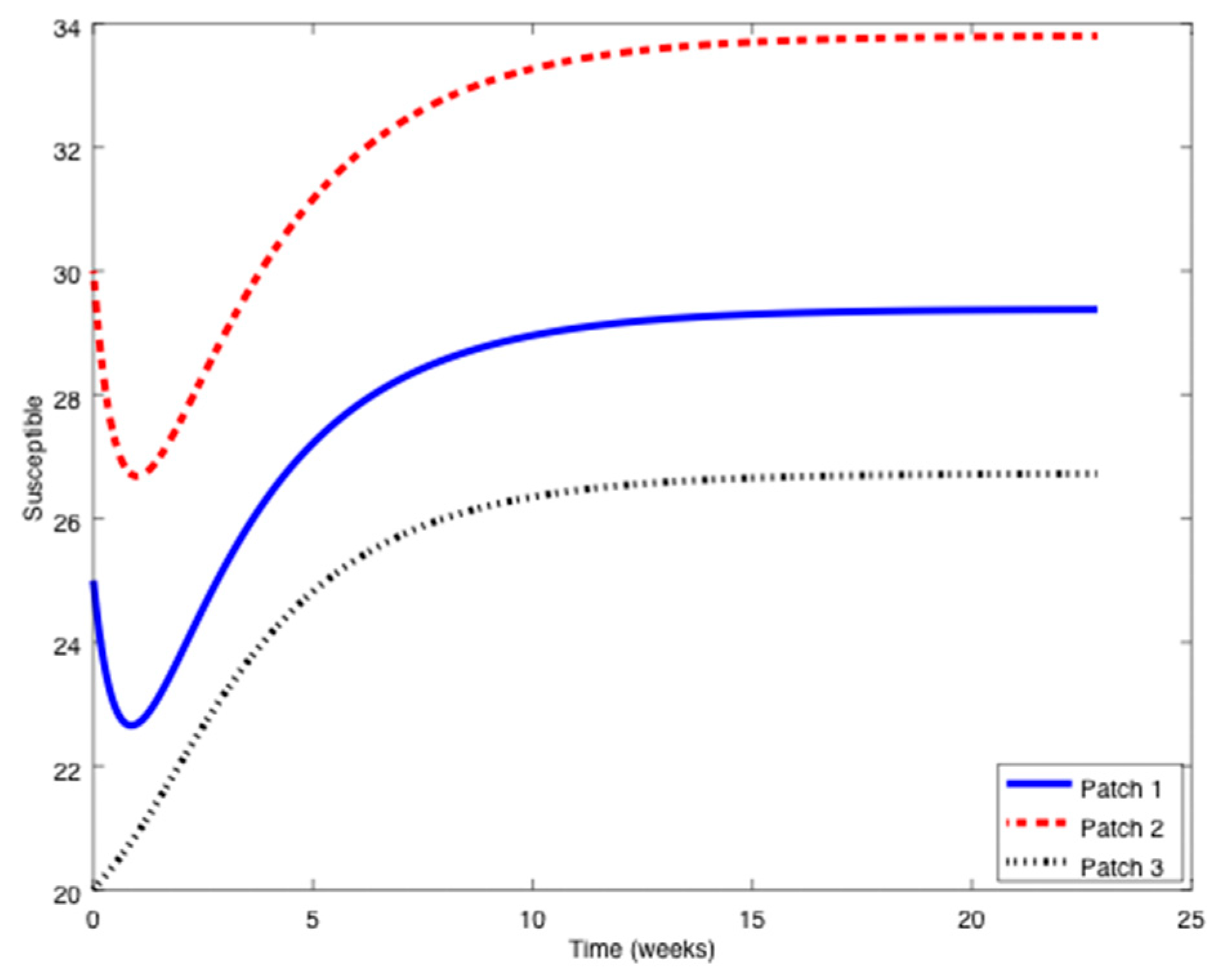
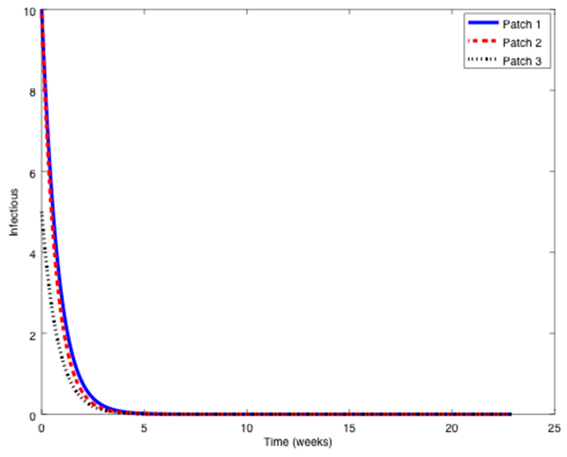
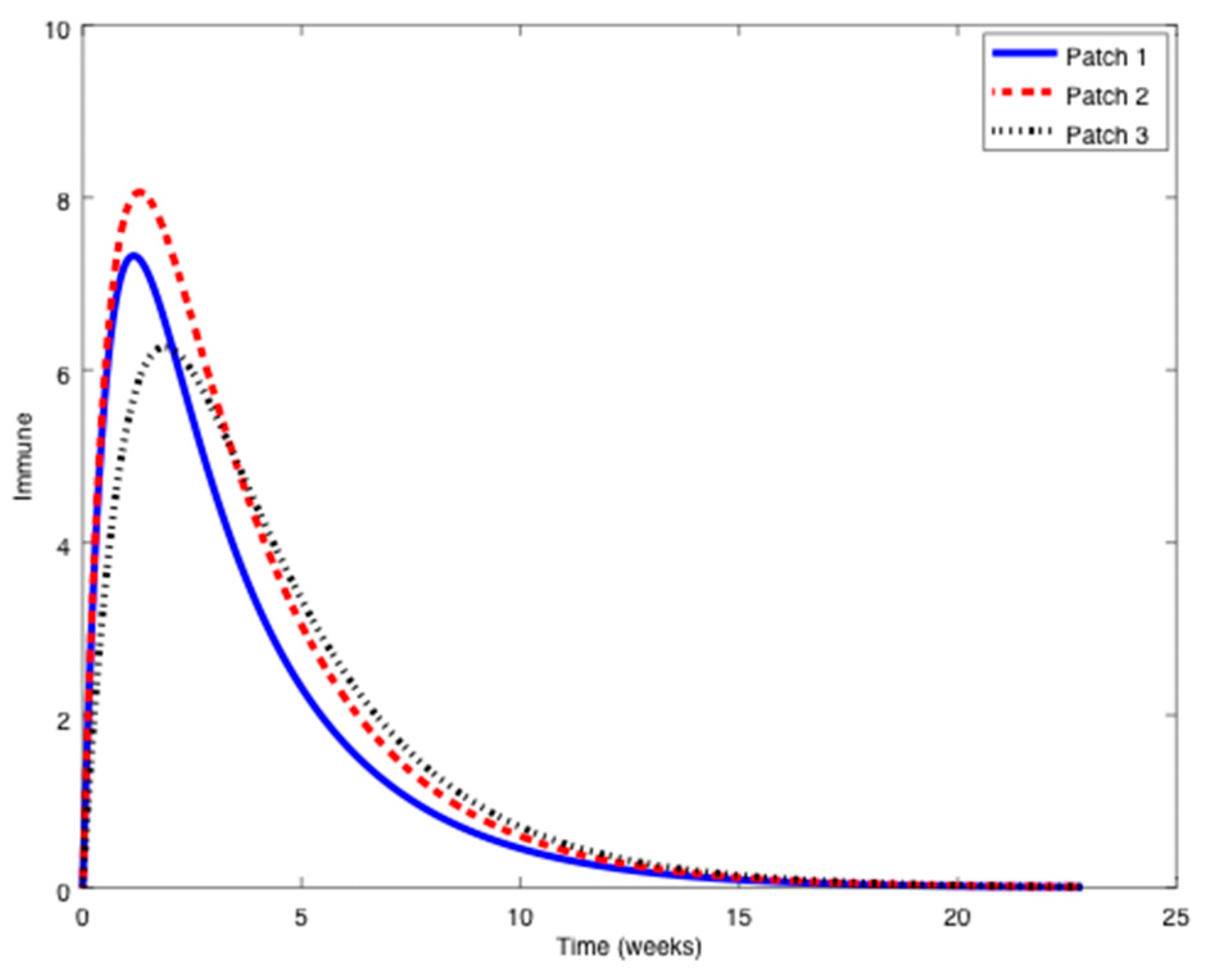
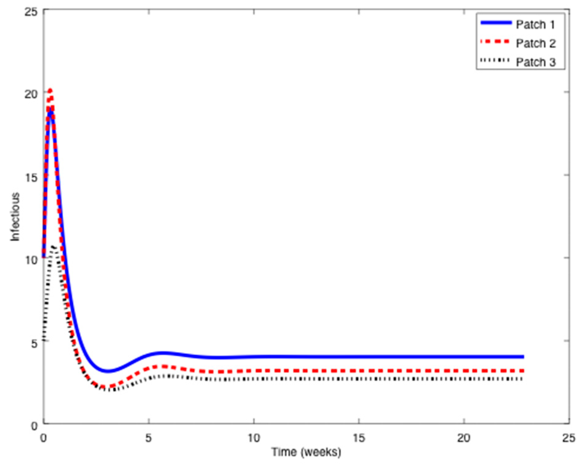
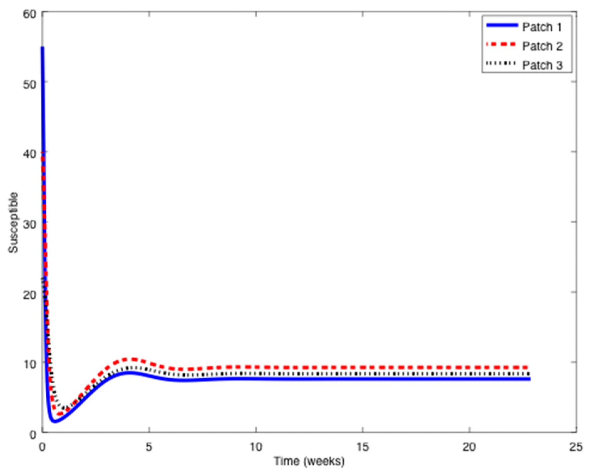
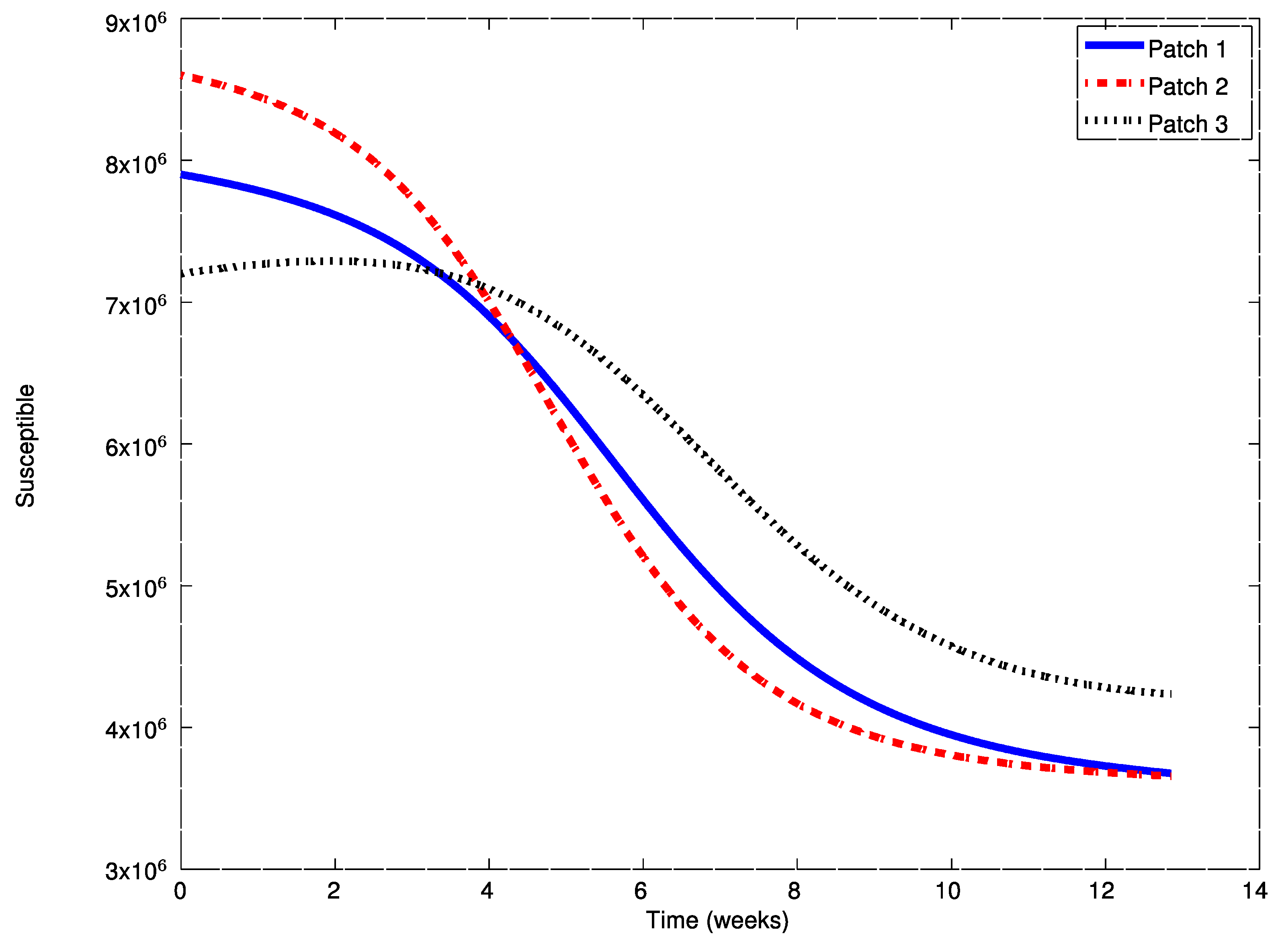
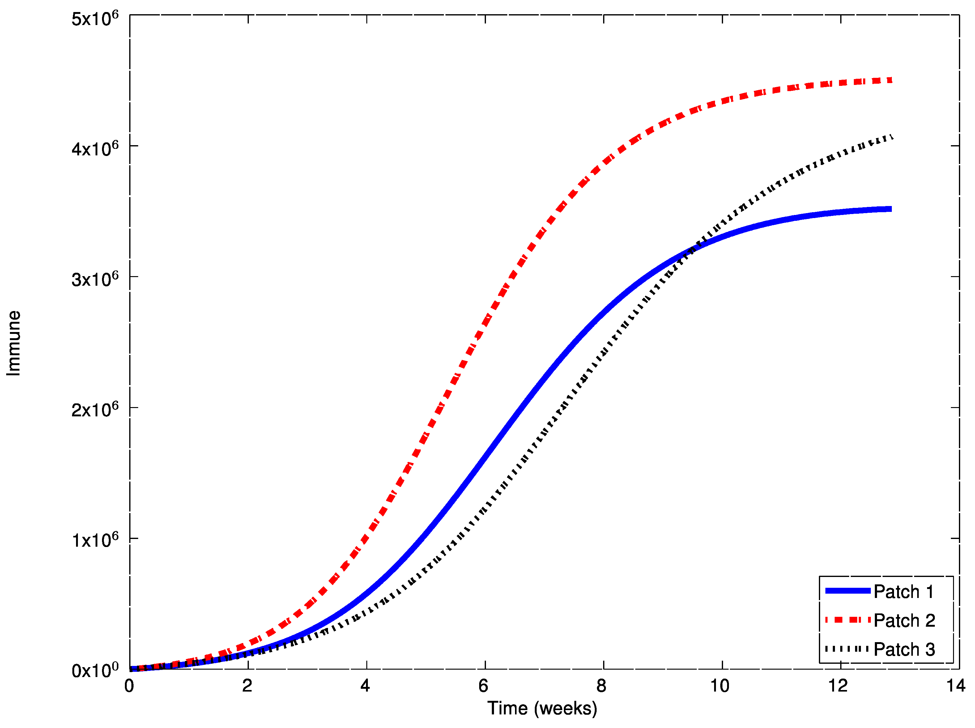
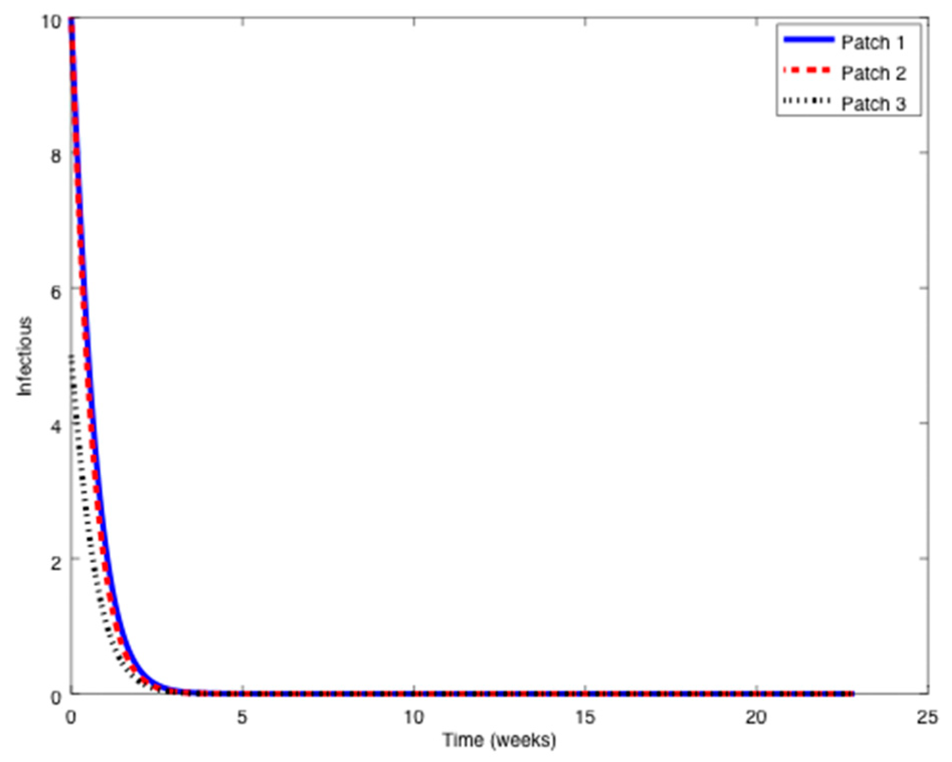
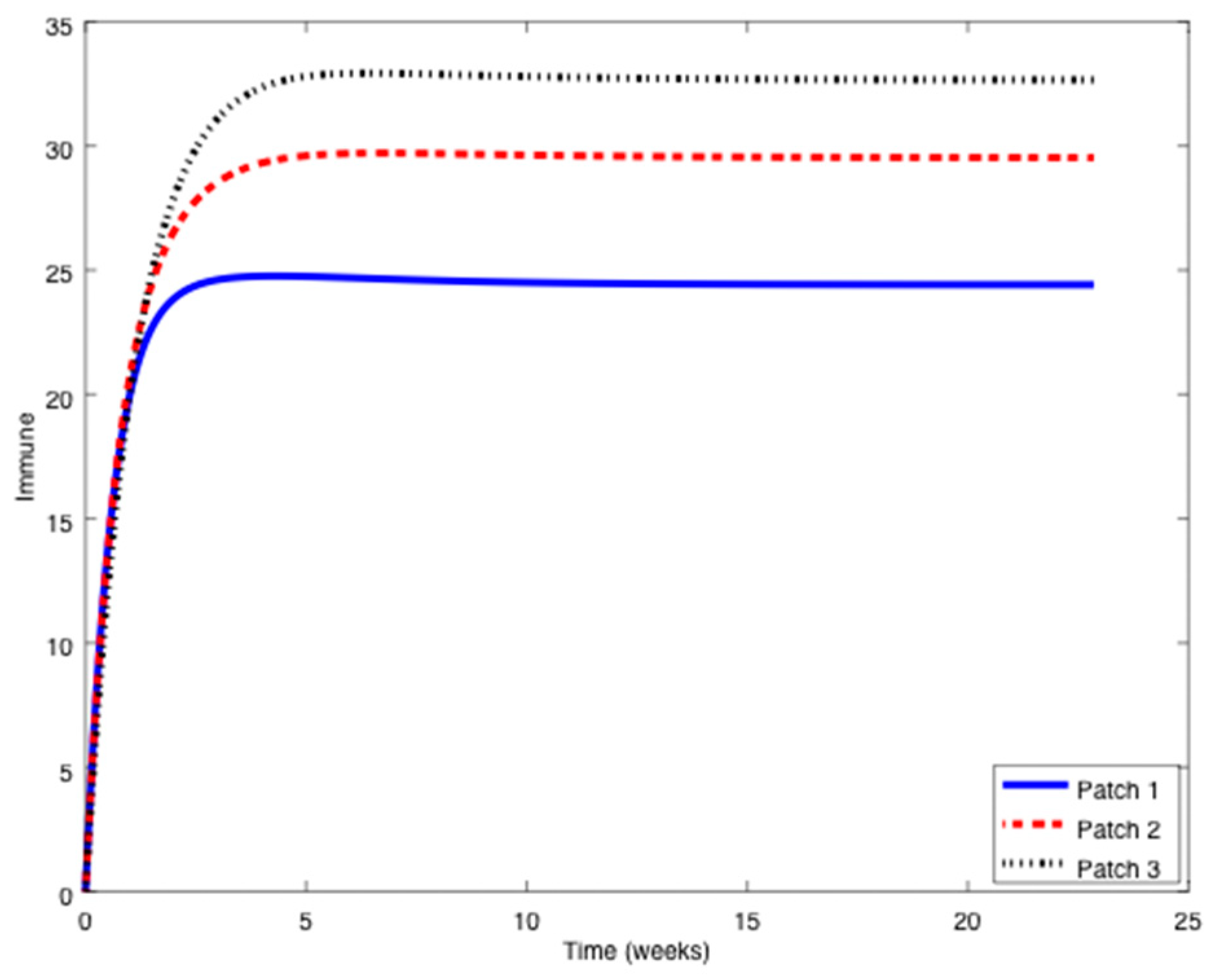
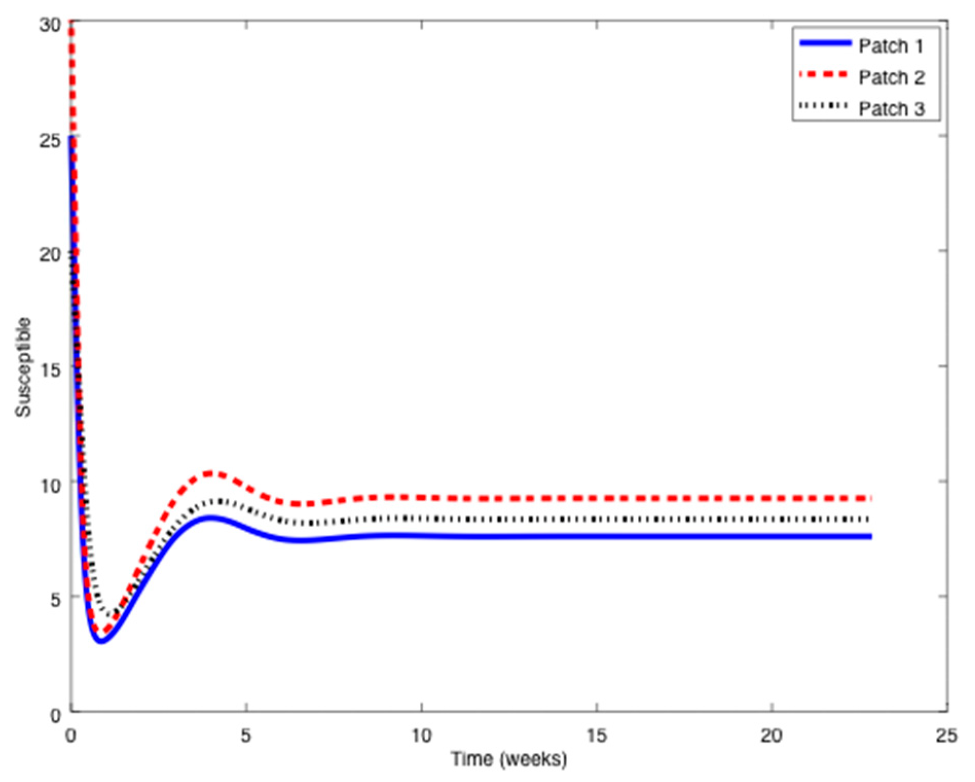
From Figure 1, Figure 2 and Figure 3 it can be observed that the above parameters correspond to the case when the reproduction number is less than unity, $R_0<1$. Thus, the solution trajectory of the system is non-negative, remains globally bounded and the disease-free equilibrium point is asymptotically stable, as claimed in Theorem 3 (iii). Moreover, $I_{dfi}=0$ and $R_{dfi}=0$ for $i=1,2,3$ while the values of $S_{dfi}$ are provided in

Table 1. Simulated and calculated values for the vaccination-free, disease-free equilibrium point.

	Theoretical Value	Simulated Value
$S_{df1}$	29.383	29.377
$S_{df2}$	33.804	33.796
$S_{df3}$	26.731	26.725

. In this way, Table 1 displays and compares the value of the equilibrium points obtained from the numerical simulation and theoretically from Equations (10) and (11).

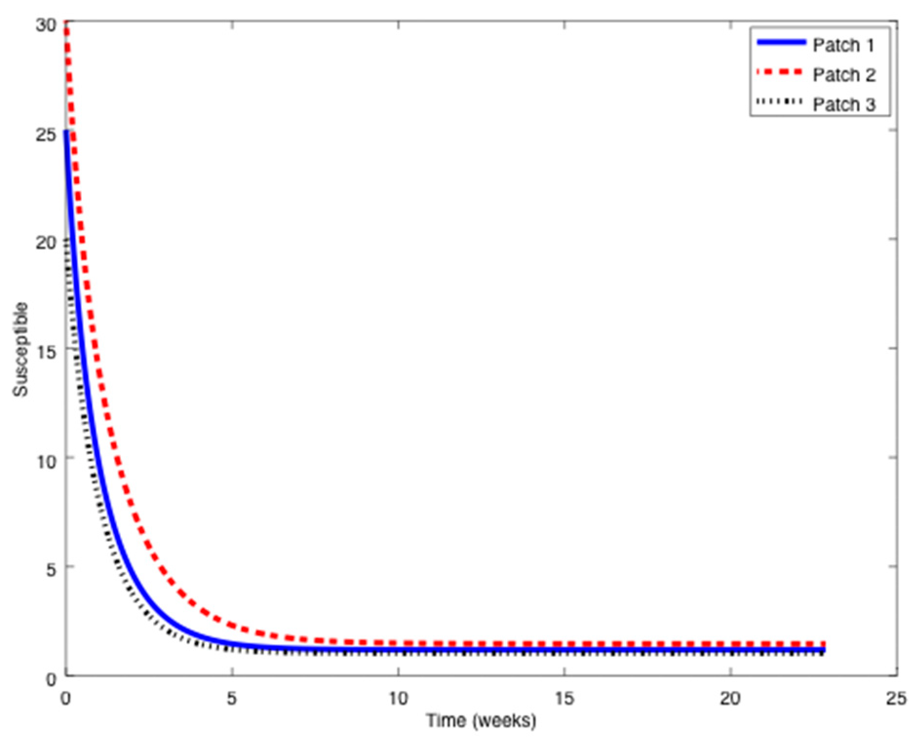
Table 1 shows a good agreement between the theoretical values and the ones obtained by simulation, confirming Theorem 1 results. The total population is given by $N_T=89.897$. Furthermore, we add now a feedback vaccination term of the form (2) with $V_0=0.9\Lambda$, $K=A$. The evolution of the system with this control action is displayed in Figure 4, Figure 5 and Figure 6.

In this case, the infectious again vanish asymptotically while the disease-free equilibrium point location is contained in

Table 2. Simulated and calculated values for disease-free equilibrium point with vaccination.

Disease-free Eqilibrium Point	Theoretical Value	Simulated Value
$S_{df1}$	1.186	1.186
$S_{df2}$	1.461	1.461
$S_{df3}$	1.027	1.027
$R_{df1}$	24.410	24.412
$R_{df2}$	29.526	29.528
$R_{df3}$	32.652	32.655

.

The total population obtained by numerical simulation is $N_T=90.268$. As it happened in the previous case, the Table 2 confirms the results provided in Theorem 1 regarding the disease-free equilibrium point location. Moreover, it is verified that the total population at equilibrium does not depend on the particular value of vaccination.

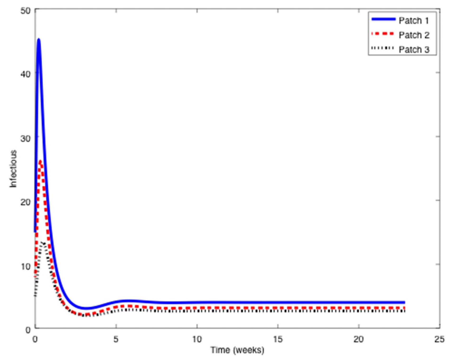
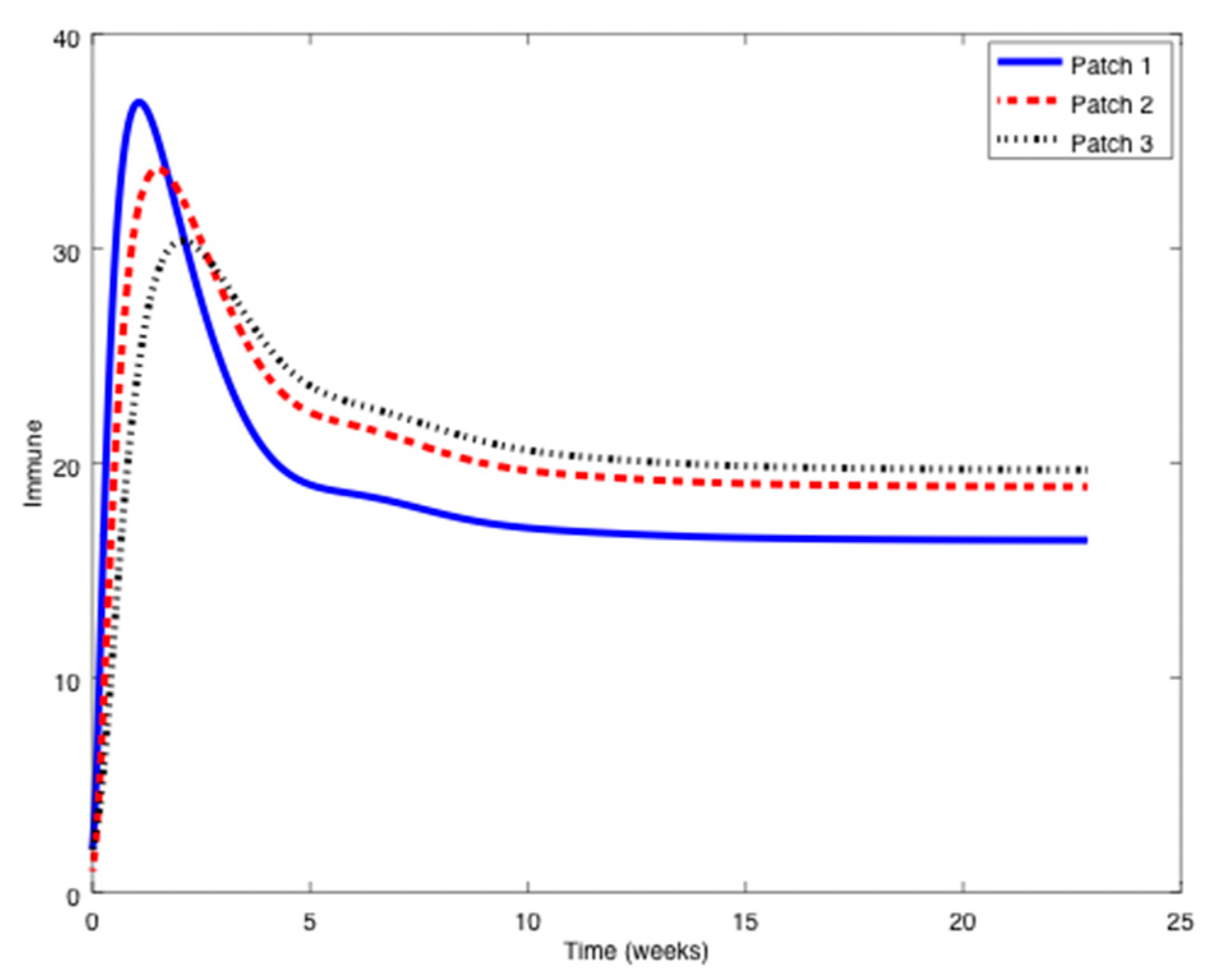
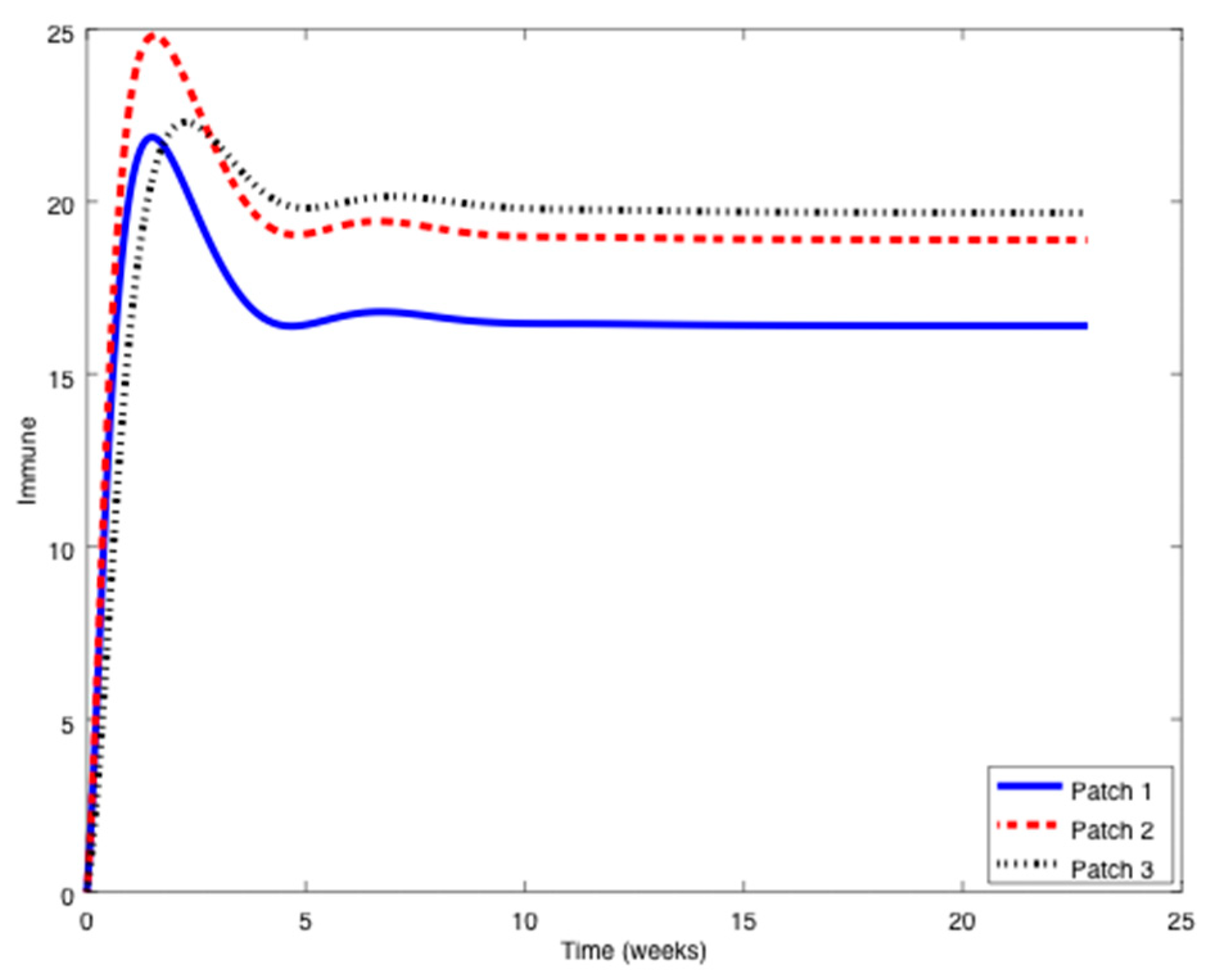
Example 2. 

Now, the value of$\beta$is increased eight times the value of Example 1 to obtain:

$$\beta =\left[{\beta }_i\right]=8\left[\begin{array}{ccc}3.24& 3.08& 3.16\end{array}\right]\times {10}^{-2}$$

so that the reproduction number is now larger than unity,$R_0>1$. In this case, the disease-free equilibrium point is unstable and an asymptotically stable endemic equilibrium point appears. The following Figure 7, Figure 8 and Figure 9 display the evolution of the system in this case when no vaccination is applied.

It can be observed that the infectious do not vanish now. The endemic equilibrium point is given by $(S_{end1},S_{end2},S_{end3})=(7.61,9.26,8.36)$, $(I_{end1},I_{end2},I_{end3})=(4.03,3.19,2.70)$, and $(R_{end1},R_{end2},R_{end3})=(16.40,18.89,19.67)$. A series of numerical experiments are conducted now to analyze the effect of parameters and initial conditions in the location of the endemic point. Thus, the initial values of the populations are now changed to:

$$\begin{gathered} S_1(0)=55;I_1(0)=15;R_1(0)=2 \\ {S}_2(0)=40;I_2(0)=8;R_2(0)=1 \\ {S}_3(0)=22;I_3(0)=5;R_3(0)=2 \end{gathered}$$

The evolution of the system with different initial conditions is shown in Figure 10, Figure 11 and Figure 12.

The endemic equilibrium point is given by the same values indicated before. Thus, the location of the endemic equilibrium point is not altered by a change in the initial values. Afterwards, the value of ${\beta }_3$ is perturbed (while the others ${\beta }_1$ and ${\beta }_2$ remain unchanged) and the location of the endemic equilibrium point for each case is provided in

Table 3. Location of the endemic equilibrium point for different values of ${\beta }_3$.

$${\mathit{\beta }}_3$$	$$({\mathit{S}}_{\mathit{e}\mathit{n}\mathit{d}1},{\mathit{S}}_{\mathit{e}\mathit{n}\mathit{d}2},{\mathit{S}}_{\mathit{e}\mathit{n}\mathit{d}3})$$	$$({\mathit{I}}_{\mathit{e}\mathit{n}\mathit{d}1},{\mathit{I}}_{\mathit{e}\mathit{n}\mathit{d}2},{\mathit{I}}_{\mathit{e}\mathit{n}\mathit{d}3})$$	$$({\mathit{R}}_{\mathit{e}\mathit{n}\mathit{d}1},{\mathit{R}}_{\mathit{e}\mathit{n}\mathit{d}2},{\mathit{R}}_{\mathit{e}\mathit{n}\mathit{d}3})$$
$28.44\times {10}^{-2}$	$(7.51,9.22,7.57)$	$(4.00,3.10,2.96)$	$(16.53,18.85,20.40)$
$37.92\times {10}^{-2}$	$(7.29,9.13,5.86)$	$(3.93,2.91,3.53)$	$(16.79,18.74,21.95)$
$63.20\times {10}^{-2}$	$(7.00,9.00,3.61)$	$(3.84,2.67,4.28)$	$(17.15,18.61,23.99)$
$94.80\times {10}^{-2}$	$(6.84,8.92,2.44)$	$(3.80,2.55,4.67)$	$(17.34,18.55,25.06)$

.

As it can be deduced from Table 3, the location of the endemic equilibrium point changes according to the change in ${\beta }_3$. To conclude this example, consider now the values of $({\beta }_1,{\beta }_2,{\beta }_3)$ included in

Table 4. Location of the endemic equilibrium point for $\beta =29.92\times {10}^{-2}$.

$$({\mathit{\beta }}_1,{\mathit{\beta }}_2,{\mathit{\beta }}_3)$$	$$({\mathit{S}}_{\mathit{e}\mathit{n}\mathit{d}1},{\mathit{S}}_{\mathit{e}\mathit{n}\mathit{d}2},{\mathit{S}}_{\mathit{e}\mathit{n}\mathit{d}3})$$	$$({\mathit{I}}_{\mathit{e}\mathit{n}\mathit{d}1},{\mathit{I}}_{\mathit{e}\mathit{n}\mathit{d}2},{\mathit{I}}_{\mathit{e}\mathit{n}\mathit{d}3})$$	$$({\mathit{R}}_{\mathit{e}\mathit{n}\mathit{d}1},{\mathit{R}}_{\mathit{e}\mathit{n}\mathit{d}2},{\mathit{R}}_{\mathit{e}\mathit{n}\mathit{d}3})$$
$(\beta ,\beta ,\beta )$	$(7.56,8.83,8.16)$	$(4.00,3.27,2.74)$	$(16.46,19.19,19.91)$
$(10\beta ,\beta ,\beta )$	$(0.83,8.37,7.31)$	$(6.09,2.98,2.20)$	$(20.95,23.52,20.87)$
$(\beta ,10\beta ,\beta )$	$(7.01,0.92,7.65)$	$(3.61,5.23,2.51)$	$(17.11,24.86,21.24)$
$(\beta ,\beta ,10\beta )$	$(6.61,8.42,0.90)$	$(3.73,2.48,5.16)$	$(17.62,18.76,26.50)$

and the corresponding endemic points.

It can be observed in Table 4 how the location of the endemic point changes as the value $10\beta$ moves from one position to another one within the vector $\left[{\beta }_1,{\beta }_2,{\beta }_3\right]$. Overall, it is concluded that the endemic point does not change with variations of initial conditions, but it generally does with parameter changes.

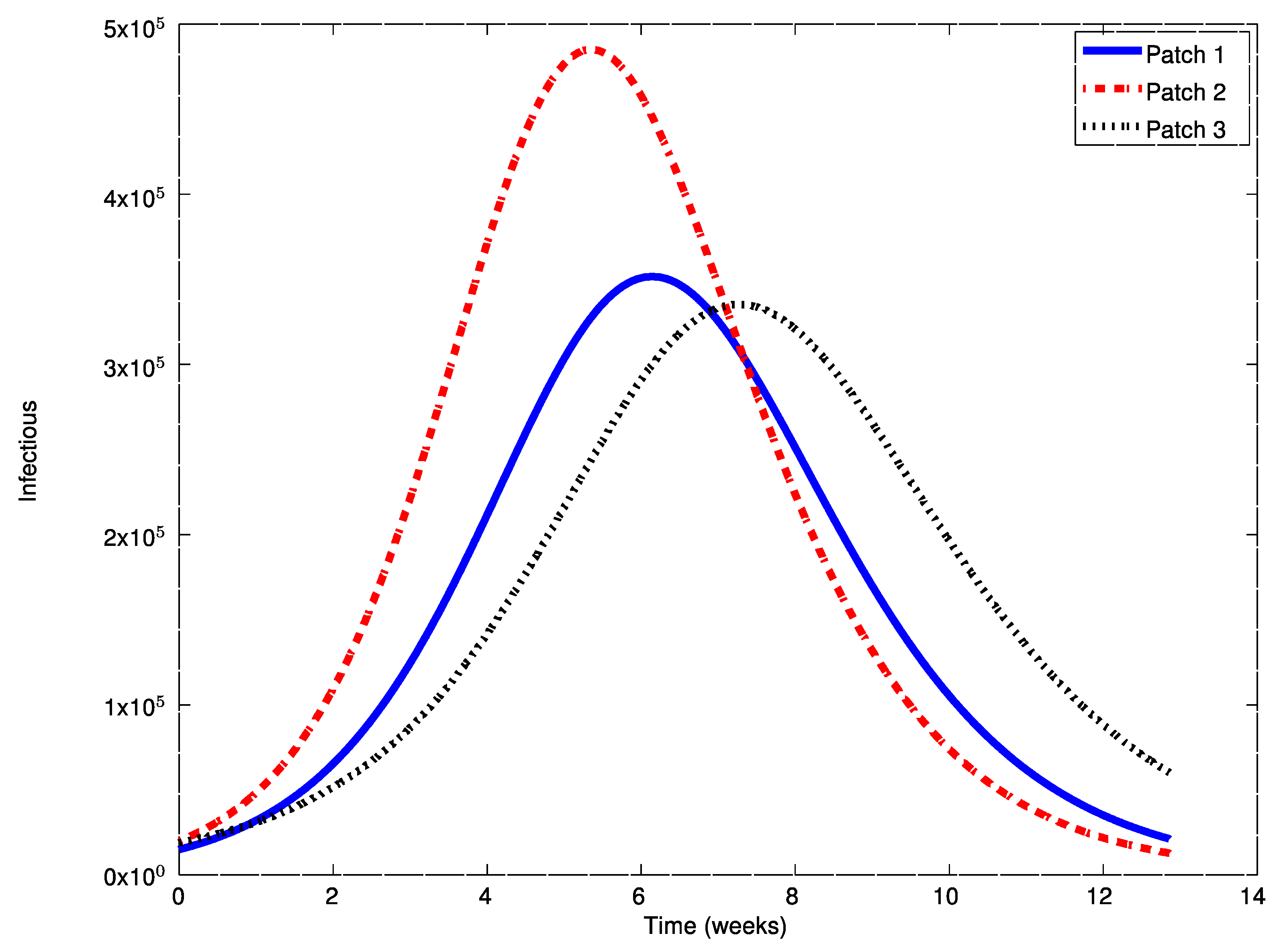
Example 3. 

Finally, consider the Hong Kong influenza epidemic in New York City in 1968–1969. This influenza outbreak is modeled by an SIR epidemic model with the following parameters [36]:

$$\beta =3.24\times {10}^{-7},\gamma =1.78$$

in units of week${}^{-1}$. The patchy environment is inspired on this real case and it is composed of three cities (or patches),$n=3$, with spreading parameters similar to the above ones and given by:

$$\begin{gathered} \Lambda =\left[{\Lambda }_i\right]=\left[\begin{array}{ccc}5& 4.5& 5.5\end{array}\right]\times {10}^3,\beta =\left[{\beta }_i\right]=\left[\begin{array}{ccc}3.24& 3.18& 3.08\end{array}\right]\times {10}^{-7} \\ {d}^X=\left[d_i^X\right]=\left[\begin{array}{ccc}1/70& 1/71& 1/72\end{array}\right]year{s}^{-1},\gamma =\left[{\gamma }_i\right]=\left[\begin{array}{ccc}1.78& 1.82& 1.75\end{array}\right] \end{gathered}$$

in units of week${}^{-1}$except otherwise indicated and thesymbol$d^X$stands for$d^S,d^I,d^R$. The initial conditions for the populations are given by the 1970 New York City census as:

$$S_1(0)=7,960,000;I_1(0)=15,000;R_1(0)=0$$

while the initial conditions for the remaining patches are given, similarly, by:

$$\begin{gathered} S_2(0)=8,600,000;I_2(0)=20,000;R_2(0)=0 \\ {S}_3(0)=7,200,000;I_3(0)=19,000;R_3(0)=0 \end{gathered}$$

The travel matrices are defined by:

$$A={10}^{-2}\times \left(\begin{array}{ccc}0& 1.2& 0.3\\ 1.1& 0& 1\\ 1.2& 1.4& 0\end{array}\right),B={10}^{-2}\times \left(\begin{array}{ccc}0& 1.12& 0.4\\ 1.22& 0& 0.85\\ 1& 1.14& 0\end{array}\right),C={10}^{-2}\times \left(\begin{array}{ccc}0& 0.78& 0.56\\ 1& 0& 0.95\\ 1.2& 0.94& 0\end{array}\right)$$

The aim of this example is to show the effect of the vaccination strategies introduced in Section 4. The evolution of the system without vaccination is displayed in Figure 13, Figure 14 and Figure 15.

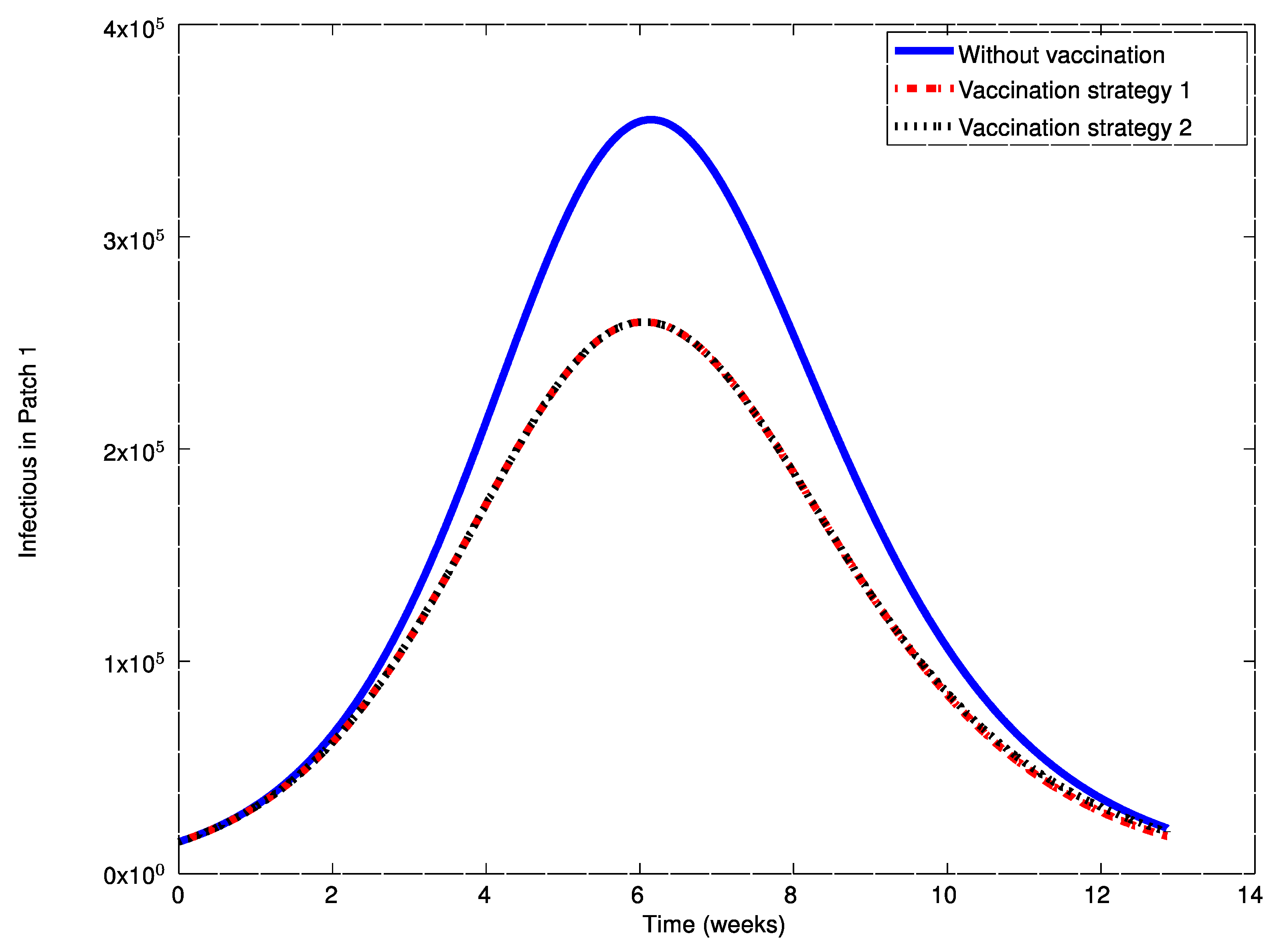
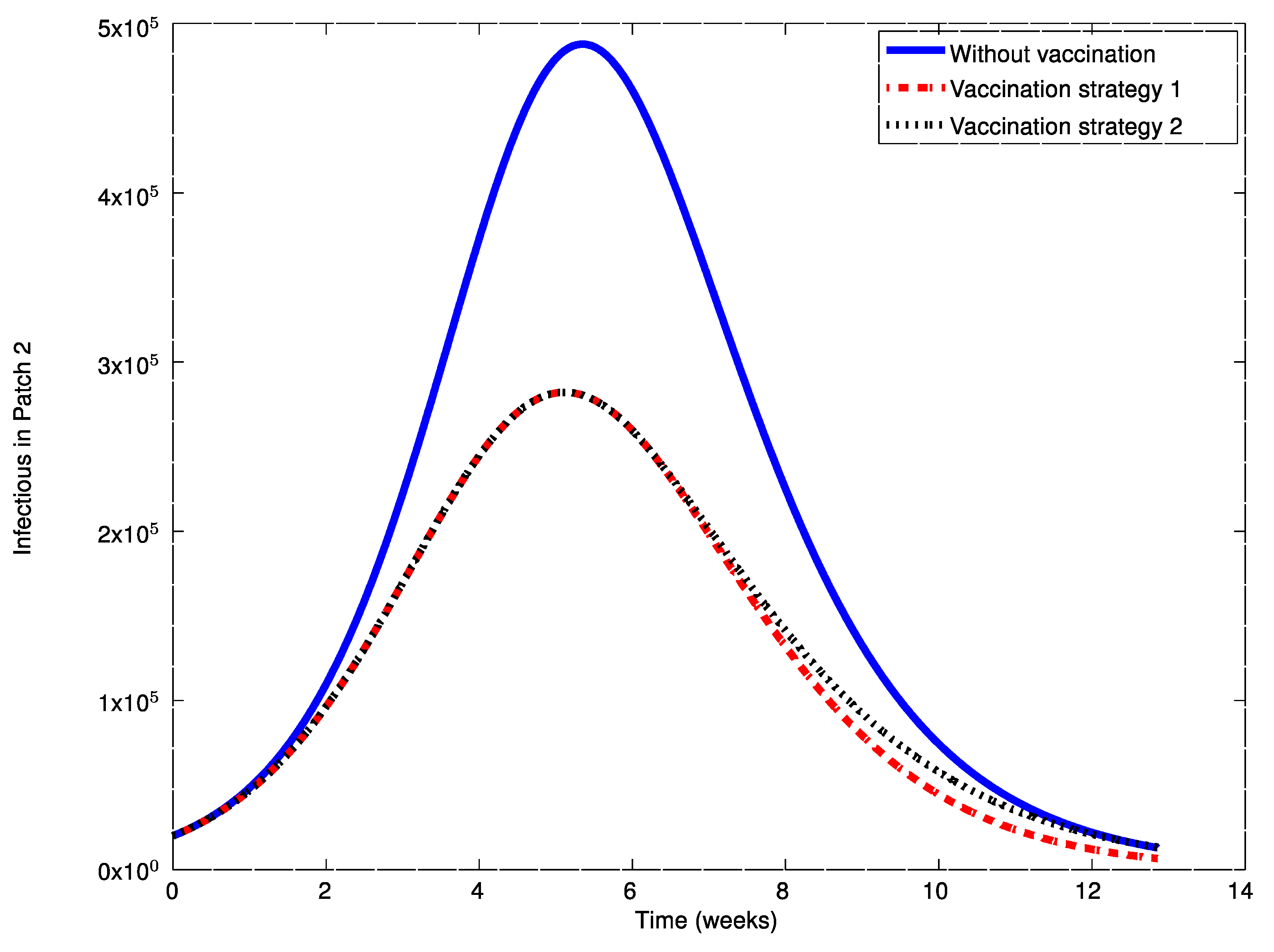
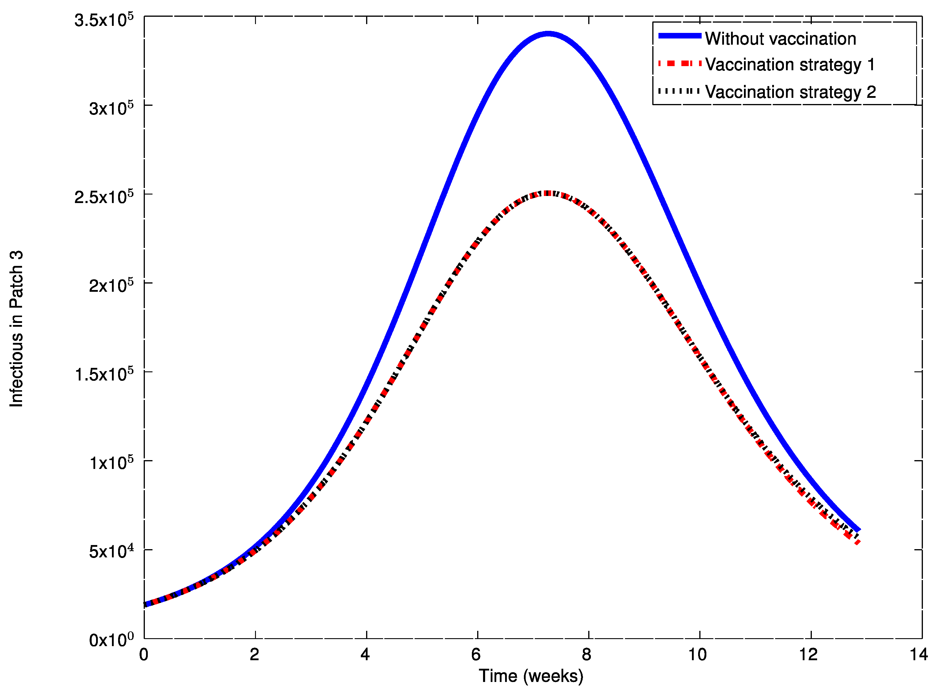
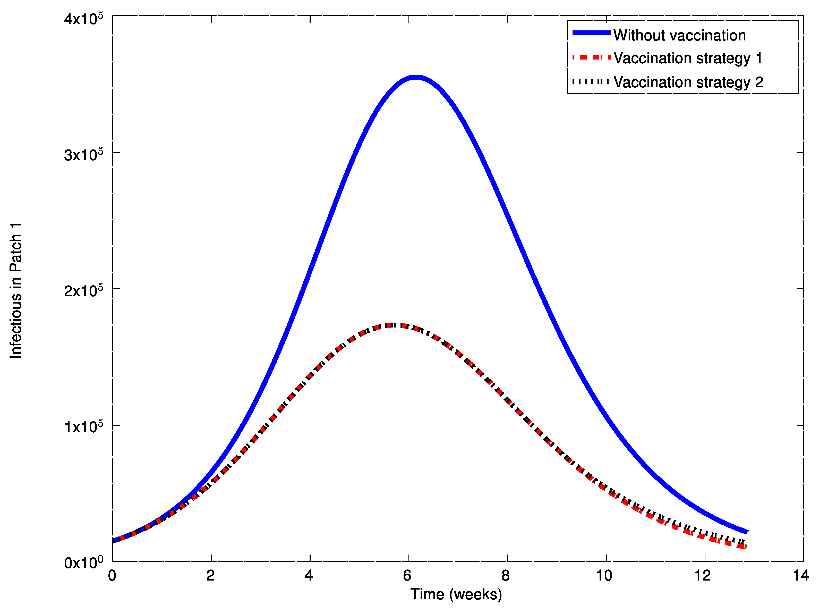
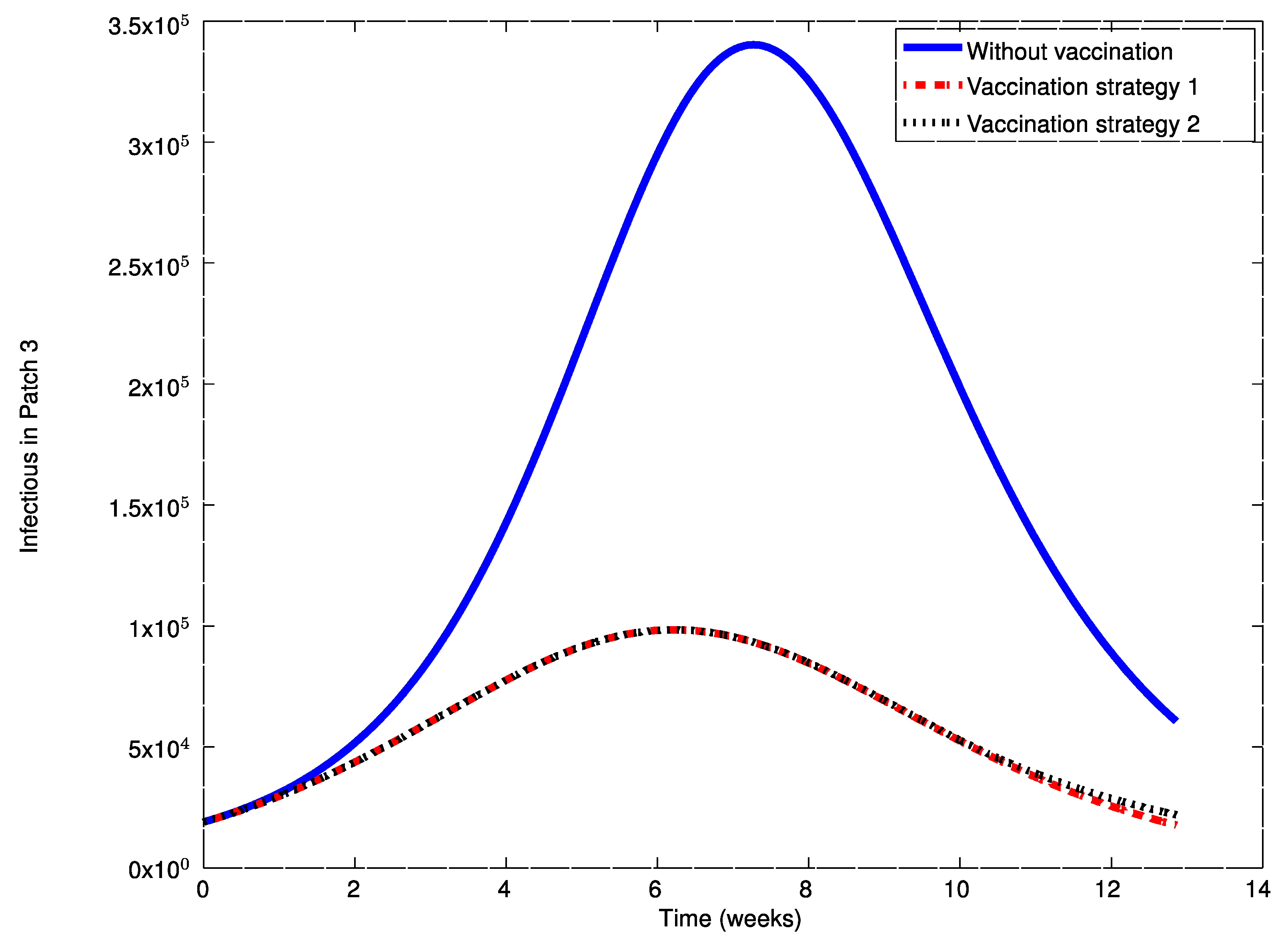
As it can be observed in Figure 14, the influenza outbreak reaches a peak during the spreading of the infection. In order to reduce the severity of the outbreak, the two vaccination strategies proposed in Section 4 are now applied and compared. To this end, consider the control matrices given by:

$$K=A+Diag\left(\left[{10}^{-2},0.6\times {10}^{-2},0.9\times {10}^{-2}\right]\right);M_i=5\times {10}^5;M_0=0.9\Lambda ;V_0=M_0$$

It can be readily seen that the above selection satisfies the constraints imposed by (30). Moreover, the thresholds to be used in Strategy 2 are given by ${\epsilon }_1=4.3\times {10}^6;{\epsilon }_2=5.1\times {10}^6;{\epsilon }_3=4.7\times {10}^6$. The Figure 16, Figure 17, Figure 18, Figure 19, Figure 20 and Figure 21 display the evolution of various infectious subpopulations in agreement with the implemented vaccination controls. The Figure 16, Figure 18, and Figure 20 show the evolution of the infectious subpopulation at each patch without vaccination and when both vaccination strategies introduced in Section 4 are employed. 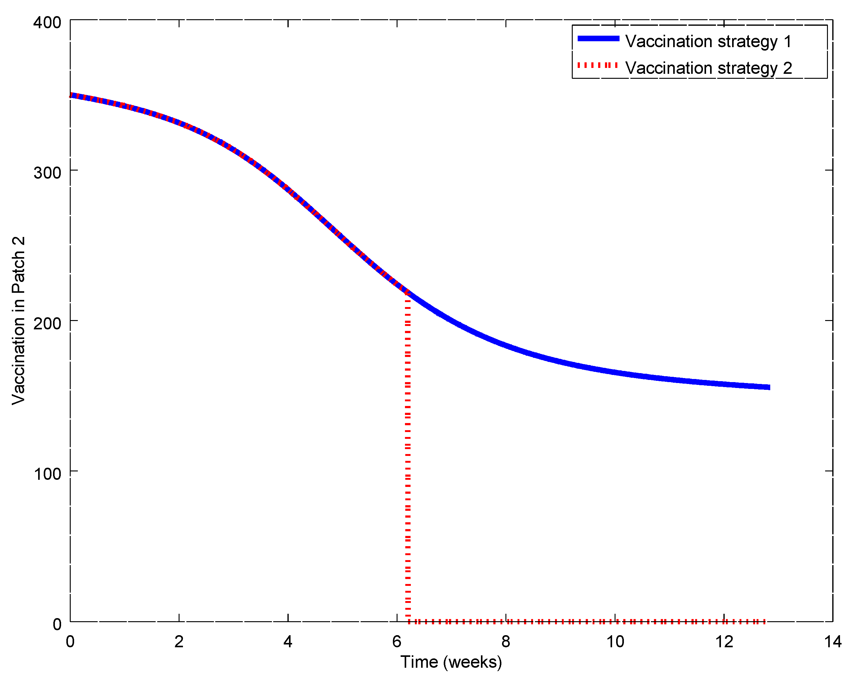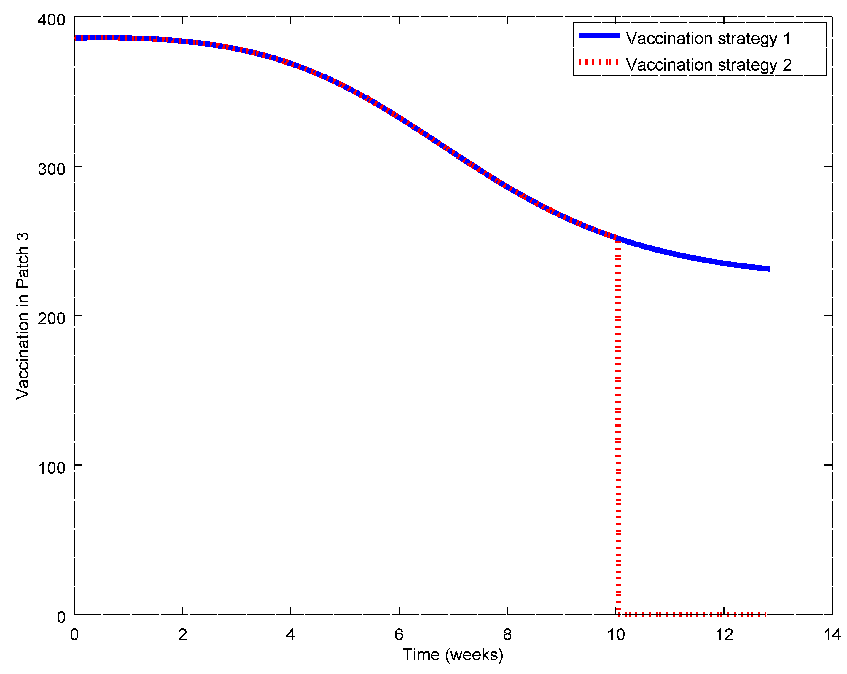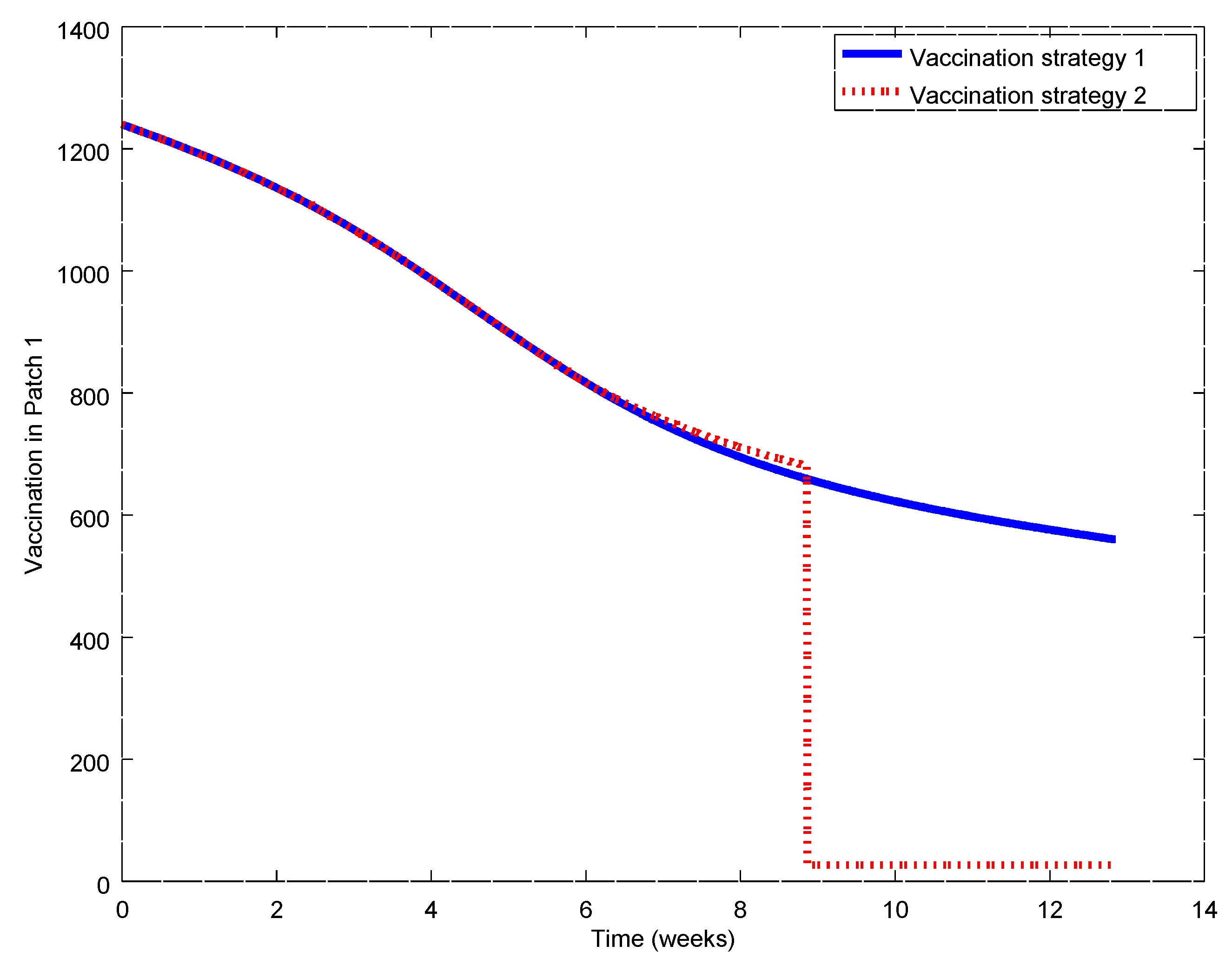Furthermore, the Figure 16, Figure 18, and Figure 20 show the vaccination commands generated by both strategies at each patch. It can be seen that the solution trajectory of the infectious is non-negative and globally bounded as it is proved in Theorem 4. From Figure 16, Figure 18, and Figure 20 it can also be concluded that the application of a judicious vaccination campaign significantly reduces the peak caused by the outbreak. 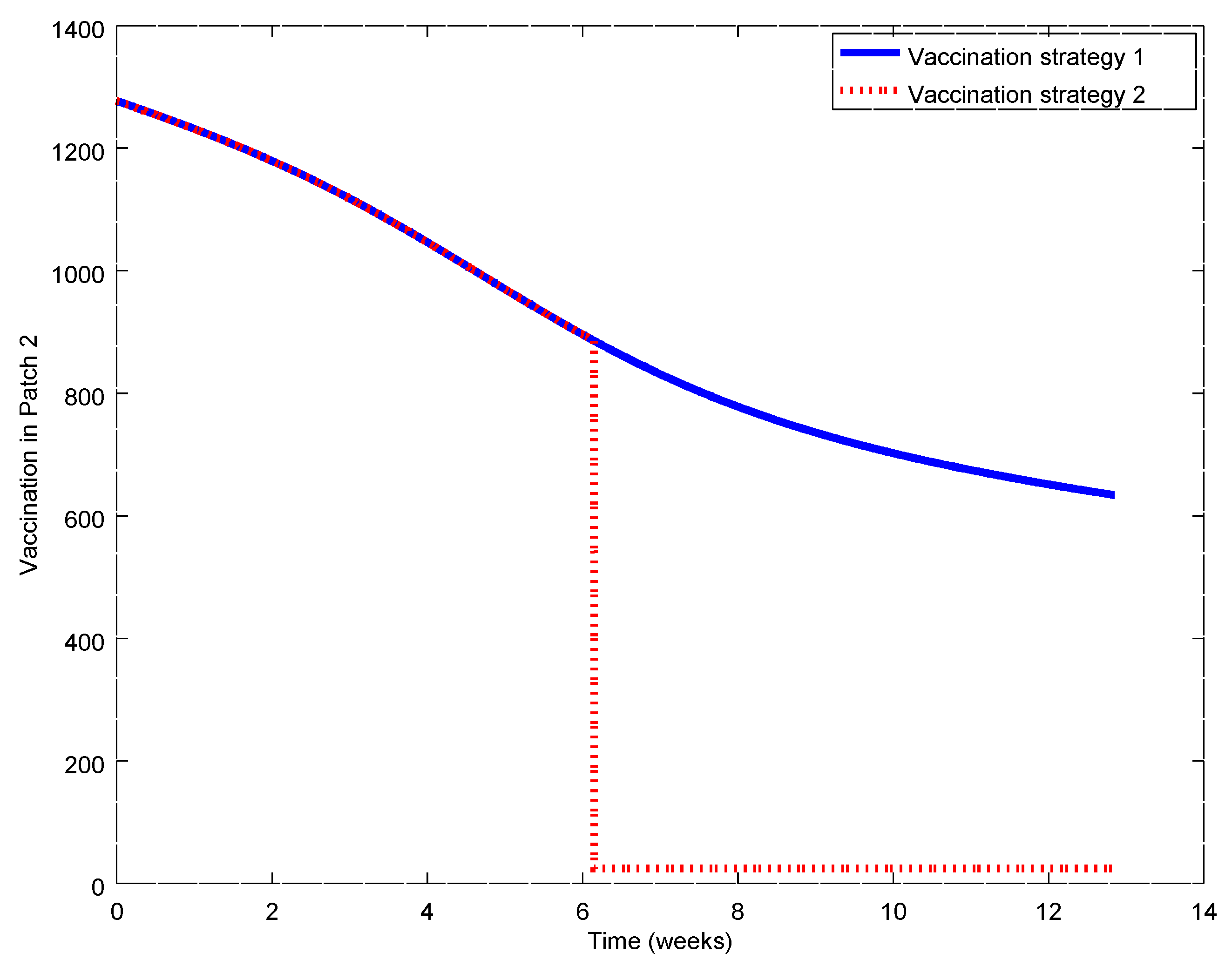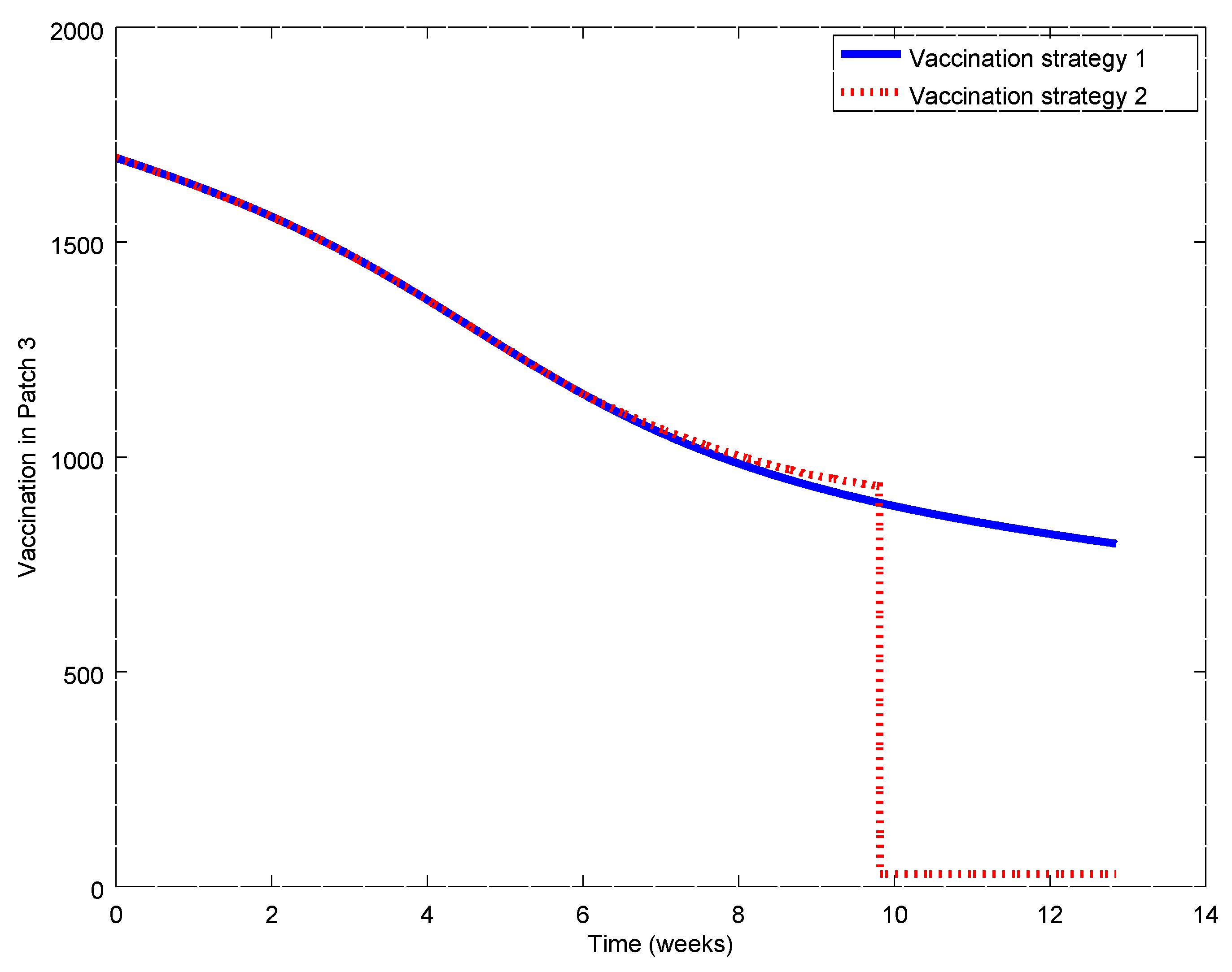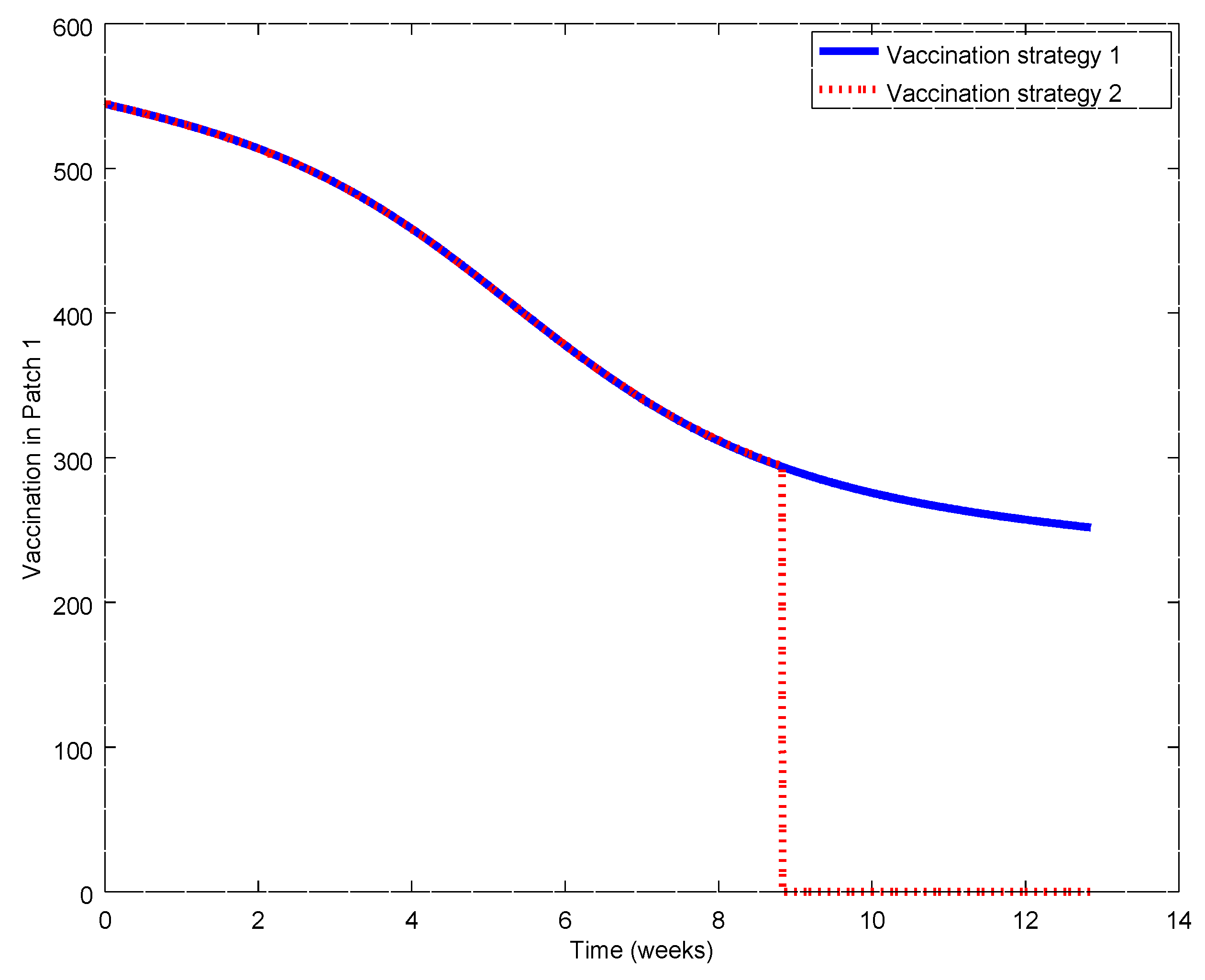In addition, Figure 17, Figure 19, and Figure 21 show that Strategies 1 and 2 generate very similar infectious subpopulation profiles, where the plots for both cases are almost superimposed. However, the vaccination law profile through time is different for Strategies 1 and 2, fact that can be observed in Figure 17, Figure 19, and Figure 21. During the first weeks, both control laws are the same but when the susceptible reach the corresponding prescribed threshold, the susceptible feedback term of Strategy 2’s vaccination law is switched off and only a constant vaccination is applied. The shutting down of the feedback term causes a noticeable decrease of the control command while the evolution of the infectious subpopulations is similar. Consequently, the vaccination Strategy 2 is able to reduce the outbreak peak, saving vaccination effort. Notice that, in this experiment, each patch disposes of full information of the remaining ones since the values of the susceptible subpopulation at the others patches are used to calculate the amount of vaccination according to Equations (31)–(33).

Now, we will change the matrix K so that it takes the following upper-triangular form:

$$K=\left(\begin{array}{ccc}{10}^{-2}& 0.1A_{12}& 0.1A_{13}\\ 0& 0.6\times {10}^{-2}& 0.1A_{23}\\ 0& 0& 0.9\times {10}^{-2}\end{array}\right)$$

In this case, the first patch has available information of the second and third patches, the second patch has only information of the third patch which has only self-information. This structure implies for the first patch, for instance, that the vaccination law considers an amount of 10% of individuals coming into the patch from the second and third ones in order to calculate the total administered vaccination. It is important to notice the difference with respect to the previous example, where all the amount of travelling individuals (coming in and going out of the patch) is considered to calculate the vaccination. The illness evolution is displayed in the various Figure 22, Figure 23, Figure 24, Figure 25, Figure 26 and Figure 27. In particular, the evolution of the infectious under these circumstances is depicted for each patch in Figure 22, Figure 24, and Figure 26. On the other hand, the vaccination generated by each one of the strategies is displayed for each patch in Figure 23, Figure 25, and Figure 27. The main conclusions drawn before regarding the effect of applying an appropriate vaccination to individuals as well as those related to the comparison of Strategies 1 and 2 hold here too. However, in this case the peak in the infectious in reduced less by applying vaccination than in the previous example. The main reason for this issue is that with the new control matrix, K, the number of administered vaccines is much lower now than in the previous case. This fact can be observed by comparing the Figure 17 and Figure 23, Figure 19 and Figure 25, and Figure 21 and Figure 27. This result shows the importance of vaccination campaigns in order to control an epidemic outbreak in a patchy environment.

6. Conclusions

This paper has considered a SIR epidemic model in a patchy environment, each patch being assumed to have its own health or medical centre. It has been assumed that there are potential travellers coming into and leaving each patch which are interchanged with the remaining patches. It has been assumed that the vaccination controls are exerted at each community health centre while either the total information or a partial information of the total subpopulations, including the interchanging ones, is shared by all the set of health centres of the whole environment under study. In this way, vaccination control laws involving constant terms and feedback information on the susceptible subpopulations have been proposed and discussed to be administrated at each health centre. In the cases that not all the information of the subpopulations distributions at other patches is known by the health centre of each particular patch, the feedback vaccination rule is considered to have a decentralized nature. Since there the control laws involved crossed gains to take into account or not (if such gains are zeroed) the couplings between patches, the vaccination action can be of either a centralized or of a (totally or partially) decentralized nature. The paper has also investigated the existence, allocation (depending on the vaccination control gains) and uniqueness of the disease-free equilibrium point as well as the existence of at least an attainable and stable endemic equilibrium point. A formal analytic characterization of the potential whole set of endemic equilibrium points has also being given based on algebraic mathematical tools for the solvability of algebraic systems of equations.