Modelling Construction Site Cost Index Based on Neural Network Ensembles

Abstract

Construction site overhead costs are key components of cost estimation in construction projects. The estimates are expected to be accurate, but there is a growing demand to shorten the time necessary to deliver cost estimates. The balancing (symmetry) between time of calculation and satisfaction of reliable estimation was the reason for developing a new model for cost estimation in construction. This paper reports some results from the authors’ broad research on the modelling processes in engineering related to estimation of construction costs using artificial intelligence tools. The aim of this work was to develop a model capable of predicting a construction site cost index that would benefit from combining several artificial neural networks into an ensemble. Combining selected neural networks and forming the ensemble-based models compromised their strengths and weaknesses. With the use of data including training patterns collected on the basis of studies of completed construction projects, the authors investigated various types of neural networks in order to select the members of the ensemble. Finally, three models that were assessed in terms of performance and prediction quality were proposed. The results revealed that the developed models based on ensemble averaging and stacked generalisation met the expectations of knowledge generalisation and accuracy of prediction of site overhead cost index. The proposed models offer predictions of cost in an accepted error range and prove to deliver better predictions than those based on single neural networks. The developed tools can be used in the decision-making process regarding construction cost estimation.

1. Introduction

The success of a construction project is determined by obtaining three fundamental goals of a project—completion within the budget, completion within planned time, and achieving the expected quality of construction works. For the budget issue, cost estimation is a key process. On one hand, the estimates are expected to be accurate; on the other hand, there is a growing demand to shorten the time necessary to deliver cost estimates. These needs justify attempts to employ various tools in fast cost analyses and modelling. The aim of this paper is to present the results of the research on artificial neural networks (ANNs) ensembles as artificial intelligence tools for fast analysis and prediction of site overhead costs. This research is a continuation and extension of previous studies, including prediction of these costs with the use of multilayer perceptron neural networks [1]. It is worth mentioning that mathematical tools—which are constantly being developed—are present in the investigations of a broad variety of problems in the field of construction management and technology. Some interesting examples are applications of fuzzy sets theory and fuzzy logic in construction project risk [2,3,4], the evaluation of a construction safety management system [5], processes in a construction enterprise [6], the investigation of flow-shop scheduling problems [7], and using multiple criteria decision-making methods for supporting the decision process in construction and building technology [8,9,10]. There have also been a number of attempts to apply artificial neural networks in the management of construction projects—predicting the completion period of building contracts [11], analysing efficiency and productivity in construction projects [12,13], predicting the maintenance cost of construction equipment [14], supporting bidding decisions [15,16], and facilitating decision making [17,18,19]. Comprehensive discussion on innovative solutions in the construction industry can be found in Reference [20].

The solutions and models that support cost estimates in construction are explored in many scientific publications. The authors propose a variety of methods, for instance multivariate regression [21], analysis of the selected cost-effectiveness factors [22], a case-based reasoning method [23], fuzzy logic [24], and genetic algorithms [25]. In terms of ANNs, there have been attempts to apply these tools in the field of construction cost management. Some examples are forecasting costs of motorways in different aspects [26], predicting cost deviations in reconstruction, alteration, and rebuilding projects [27], estimating the costs of construction projects [28,29], cost estimates of residential buildings [30], prediction of overhead costs [31,32], cost estimates of buildings’ floor structural frames as a higher level of aggregation elements of building information model [33], construction cost of sports fields [34], and shovel capital cost estimation [35].

According to the research presented in Reference [36], the influence of an improper calculation of the overhead costs can create a significant negative financial situation for the contracting company. Generally, the building contractor’s overhead costs are divided into two categories—site (project) overhead costs and company’s (general) overhead costs [37]. The site (project) overhead costs include items that can be identified with a particular job, but not materials, labour, or production equipment. The company’s overhead costs are items that represent the cost of doing business and are often considered fixed expenses that must be paid by the contractor. On the other hand, an overhead cost of a construction project can be defined as a cost that cannot be identified with or charged to a construction project or to a unit of construction production [38]. A new classification of construction companies into competitiveness classes according to the relative value of overhead costs was proposed in Reference [39]. As far as accuracy is concerned, it is more advantageous to calculate both components separately—as is done in Great Britain [40], the US, and Canada [41]. The unstable construction market makes it difficult for construction companies to decide on the optimum level of overhead costs [42].

A number of empirical studies relate to the determination of the project overhead costs. In Reference [43], it is indicated that the method of work is a critical factor affecting the amount spent on project overheads. In Reference [44], the authors pointed that the location of the site could affect a number of project overhead items. In References [31,45,46], research carried out in different countries allowed for the identification of different factors that should be taken into account in site (project) overhead costs.

Studies on construction project overheads and factors that influence their estimates report that it is difficult to determine unambiguously which of the cost components are of the highest importance. Most attention is paid to a detailed calculation of site overheads; however, it is a time-consuming task to take into account all of the possible components of site overhead costs [36].

The aim of the authors’ work was to develop a regression model based on the ANNs ensembles, capable of the prediction of site overhead cost index, and, thus, able to support the estimation of site overhead costs in construction projects. An additional research objective was to explore the capabilities of ANNs ensembles in this problem. In the application of ANNs, a very common approach is to select one network to be the core of a developed model. The selection is preceded by a training and performance assessment of numerous networks—compare, e.g., Reference [47]. As an alternative, the employment of a combination of networks i.e., ANNs, offer significant capabilities. Despite their advantages, the ANNs ensembles are rarely reported on for the prediction of widely understood construction costs in research papers.

Site overhead costs can be estimated with the use of preliminaries (compare References [40,41])—such a method is accurate but time-consuming as all of the cost items must be assessed separately. On the other hand, index methods (compare Reference [36]) allow for quick estimation of site overhead costs, however the accuracy depends on the assumption of the index. The novelty of the approach proposed in this paper relies on the use of knowledge and information from the completed construction projects to train several neural networks, combine them into an ensemble, and assess the site overhead costs on the basis of the predictions produced by the ensemble of neural networks.

The paper content includes an introduction and review of the literature in the above section. Section 2 presents the theoretical background of the problem, and a discussion of the site overhead cost index prediction as a regression problem is presented in Section 3. In Section 4, the authors propose a methodology for the implementation of an ensemble of neural networks (with the use of ensemble averaging and stacked generalisation approaches) for prediction of site overhead cost index, present the results of the studies, and discuss the results. Section 5 includes a summary and conclusions.

2. Background of The Problem, Methods, and Main Assumptions

The development of the proposed model comes down to solving a regression problem and approximation of the true regression function, which is the relationship between the site overhead costs index (as the dependent variable of the model) and a set of selected predictors (as independent variables of the model). The theory of ANNs is widely presented in the literature—for instance, References [47,48,49]. ANNs, as mathematical tools applied in regression problems, offer an approximation of the true regression function g(x_j) of multiple variables x_j where j = 1,…,n:

$$g(x_j)=f(x_j)+\epsilon ,$$

(1)

In the equation (1), function f(x_j), as an approximation of g(x_j), is assumed to be implemented implicitly by a trained single ANN, selected from a number of trained candidate networks, where ε denotes an error of approximation. There are two disadvantages of an approach based on the selection of a single ANN and discarding the rest of the candidate networks [47,48]—the effort required for the training and assessment of the number of candidate networks is wasted. Moreover, the generalisation performance of the chosen network is biased with respect to some part of the input space due to the selection of learning, testing, and validating subsets from the overall number of patterns available for the training process, structure of the network, its parameters, and conditions of training process initialisation. An alternative approach is to combine a number of different ANNs that share common input x_j and form an ensemble (the ANNs may differ in their structures, parameters, and way of training, and the ensemble may even include different kinds of networks). In this paper, the authors consider two alternative approaches that are based on ensembles of neural networks—the first approach is termed as ensemble averaging, and the second one stacked generalisation—compare, e.g., References [47,48]. In the next three subsections, the authors systematically present the background of the research and the main assumptions of the model development process.

2.1. Ensemble Averaging

The main assumption for the ensemble averaging approach is that approximation of g(x_j) is done with the use of a linear combination of K-trained ANNs. The formal notation is given by Equation (2):

$$g\left(x_j\right)=\frac{1}{K}{\sum }_{i=1}^K{f}_i\left(xj\right)+{\epsilon }_i,$$

(2)

where f_i(x_j) stands for the approximation and ε_i denotes an error of approximation by i-th neural network for i = 1,…,K. Such a mechanism (compare Reference [48]), which does not involve input signals, where individual outputs of ANNs are combined to produce an overall output, belongs to a class of static structures. The following assumptions can be made [47]—the sum-of-squares error for f_i(x_j) can be given as:

$$E_i^{sos}=\sum \left({\left\{g\left(x_j\right)-f\left(x_j\right)\right\}}^2\right),$$

(3)

where E_i^sos corresponds to an integration over x_j, weighted by unconditional density p(x_j):

$$E_i^{sos}\equiv \int \dots \int \dots \int {\epsilon }_i{}^2\left(x_j\right)p\left(x_j\right)d{x}_1\dots d{x}_j\dots d{x}_n,$$

(4)

The average error by the networks acting individually can be written as

$$E_{av}^{sos}=\frac{1}{K}{\sum }_{i=1}^K{E}_i^{sos}.$$

(5)

Supposing that the output of the ensemble of networks is the average of outputs of K networks that belong to the ensemble, we have the prediction of the ensemble f_ens(x_j):

$$f_{ens}\left(x_j\right)=\frac{1}{K}{\sum }_{i=1}^K{f}_i\left(x_j\right).$$

(6)

Under the assumption that ε_i(x_j) are uncorrelated and have zero mean, the relation of the ensemble error to the average error of the networks working separately is:

$$E_{ens}^{sos}=\frac{1}{K^2}{\sum }_{i=1}^K{E}_i^{sos}=\frac{1}{K}{E}_{av}^{SOS}.$$

(7)

In practice, ε_i(x_j) are highly correlated and the reduction of the error is much smaller. Typically, some useful reduction of the error is obtained, as the ensemble averaging cannot produce an increase in the expected error:

$$E_{ens}^{sos}\le E_{av}^{SOS}.$$

(8)

The expectation is that differently trained networks converge to different local minima on the error surface, and the overall performance is improved by combining the outputs in some way [47]. The employment of neural networks ensembles may lead to satisfactory results, especially when the number of training patterns is relatively low or the training data is noisy [47,50].

2.2. Stacked Generalisation

The stacked generalisation approach, (compare Reference [47]), is based on combining several trained networks together into a two-level model. The general expectation of such an approach is to improve the generalisation capabilities of the networks acting in isolation. The two-step procedure includes a training set of K level-0 networks, whose outputs are then used to train a level-1 network. One can say that the level-0 networks form an ensemble, and the level-1 network acts as a combiner of the outputs of the networks belonging to the ensemble. The general idea of the approach is presented in Figure 1.

A stacked generalisation-based model combines the outputs of level-0 networks trained with the x_j inputs; the outputs of level-0 networks can be written down as ${\widehat{y}}_i$ = f_i(x_j), with the use of the level-1 network to give the final output. Formally the model can be given as

$$\mathit{g}\mathbf{\left(}{\mathit{x}}_{\mathit{j}}\mathbf{\right)}\mathbf{=}\mathit{h}\mathbf{\left(}{\mathit{f}}_{\mathit{i}}\mathbf{\left(}{\mathit{x}}_{\mathit{j}}\mathbf{\right)}\mathbf{\right)}\mathbf{+}{\mathit{\epsilon }}_{\mathit{s}\mathit{g}}.$$

(9)

Consequently, predictions on new data is also a two-step procedure. They are made by presenting new input data to the level-0 networks and computing their outputs, which are then presented to the level-1 network which computes the final output. The general suggestion for the stacked generalisation approach is that the ensemble of level-0 networks should consist of various networks that differ from each other, whilst the level-1 network should have a relatively simple structure [47].

3. Construction Site Overhead Cost Index Prediction as a Regression Analysis Problem—Assumptions for Ensemble Averaging and Stacked Generalisation

The prediction of site overhead cost index by the neural networks ensemble and ensemble averaging approach can be formally given with the following Equations (10) and (11):

$$y=\frac{1}{K}{\sum }_{i=1}^K{f}_i\left(xj\right)+{\epsilon }_i,$$

(10)

$${\widehat{y}}_{ens}=\frac{1}{K}{\sum }_{i=1}^K{f}_i\left(xj\right),$$

(11)

where y—real life values of site overhead cost index (dependent variable), ${\widehat{y}}_{ens}$—values of y predicted by the ensemble of neural networks, f_i—the i-th mapping function implemented implicitly by the i-th neural network belonging to an ensemble, x_j—dependent variables, input shared by all of the members of the ensemble for j = 1,…,m, ε_i—error of approximation by the i-th member of the ensemble for i = 1,…, K.

On the other hand, the prediction by neural networks ensemble and stacked generalisation approach is denoted with Equations (12) and (13):

$$y=h\left(f_i\left(x_j\right)\right)+{\epsilon }_{sg},$$

(12)

$${\widehat{y}}_{sg}=h\left(f_i\left(x_j\right)\right),$$

(13)

where y—as in (11), ${\widehat{y}}_{sg}$—values of y predicted by the stacked generalisation-based two-level model, h—the mapping function implemented implicitly by level-1 neural network, f_i—the i-th mapping function implemented implicitly by i-th level-0 neural network, x_j—as in (11), and ε_sg—the error of approximation by the model.

The relationship between the set of selected predictors and the site overhead cost index was investigated by the authors. Eleven independent variables of the model were selected on the basis of studies of literature [28,31,46] and investigations of the number of projects completed in Poland. The training data included samples of real-life values of dependent variables, y, and corresponding vectors of dependent variables, x_j. The value of the dependent variable in the p-th sample (p = 1,…,143) was calculated as follows:

$$y^p=SO{C}_{ind}{}^p=\frac{SO{C}^p}{L{C}^p+M{C}^p+E{C}^p+S{C}^p}\cdot 100\%,$$

(14)

where SOC_ind^p—site overhead costs index, SOC^p—site overhead costs observed in reality, LC^p—labour costs observed in reality, MC^p—material costs observed in reality, EC^p—equipment costs observed in reality, and SC^p—subcontractors’ costs observed in reality for the p-th observation (sample). Some exemplary data, including cost components present in the Equation (13), in thousands of Euros, and corresponding site overhead cost indexes, are presented in

Table 1. Exemplary values of site overhead costs index.

p	SOCp	LCp	MCp	ECp	SCp	SOCindp
11	450.00	3828.60	4183.50	336.00	1818.40	4.4%
37	289.00	1693.00	1564.00	85.00	0.00	8.6%
72	812.54	3393.91	2893.45	564.30	5146.69	6.8%
99	217.60	382.36	514.23	48.52	547.43	14.6%

.

Independent variables of the model were selected on the basis of studies of the literature and investigations of the number of projects completed in Poland. As a result, a set of selected independent variables was proposed; these variables were denoted as x_j, where j = 1,…,11. Three variables brought to the model information about the types of work that were executed in the project were:

• x₁—types of work—general construction works,
• x₂—types of work—installation works,
• x₃—types of work—engineering works.

Another four variables brought to the model information about the construction site location were:

• x₄—construction site location—in the city centre,
• x₅—construction site location—outside the city centre,
• x₆—construction site location—non-urban spaces,
• x₇—distance between the construction site and the company’s office.

One of the variables brought to the model information about the duration of construction works was:

• x₈—overall duration of construction works.

Another two variables brought to the model information about the execution of works in winter and about the subcontracted works were:

• x₉—relationship between the amount of works performed in winter to the total amount of works,
• x₁₀—relationship of the amount of works performed by subcontractors to the total amount of works.

The last variable brought to the model information about the main contractor was:

• x₁₁—size and necessary potential of the main contractor.

(When compared to the earlier authors’ studies on the problem [1,32], the set of ten independent variables has been expanded. Thorough review of available data, which was collected in the earlier phases of the research, allowed to select an additional variable which brings to the model information about the capabilities of the contractor - namely its size and potential.)

Variables x₁–x₆ were of the nominal type. A binary method of coding was applied in the case of x₁, x₂ and x₃—their values range was 0 or 1. In the case of x₄, x₅ and x₆—a “1 of n” method of coding was applied—the range of values, considered for the three variables altogether, was 1, 0, 0 or 0, 1, 0 or 0, 0, 1.

Variables x₇–x₁₀ were of the quantitative type, whereas x₁₁ was of the nominal type. A pseudo-fuzzy scaling method of coding was applied for transformation of the original values or information into numerical values into the range 0.1–0.9 in the case of the variables presented in

Table 2. Transformation of the descriptive values into the numerical values for variables x₇–x₁₁.

Variable	Description	Descriptive Values	Numerical Values
x7	distance	up to 20 km	0.1
		more than 20 km	0.9
x8	duration of construction works	up to 6 months	0.1
		between 6 and 12 months	0.5
		more than 12 months	0.9
x9	share of the amount of works executed in winter	up to 10%	0
		between 10% and 20%	0.1
		between 20% and 40%	0.3
		between 40% and 60%	0.5
		between 60% and 80%	0.7
		between 80% and 90%	0.9
		more than 90%	1
x10	share of subcontractors in the total amount of works	up to 20%	0.1
		between 20% and 50%	0.5
		between 50% and 100%	0.9
x11	size and potential of the main contractor	low	0.1
		average	0.5
		high	0.9

, but for the variable x₉ the values were scaled into the range 0.0–1.0. The transformation for these variables is presented in Table 2. The rationale for the transformation was to provide a common scale for all of the variables.

The database that included 143 samples was built on the basis of a survey which was completed by Polish contractors. The survey investigated the factors that influence site overhead costs and the scope and complexity of construction works for completed building projects. The studies of the returned surveys resulted in gathering and ordering data used in the process of ANNs training.

Table 3. Exemplary samples of the training data.

p	x1	x2	x3	x4	x5	x6	x7	x8	x9	x10	x11	y
7	1.00	0.00	0.00	0.00	1.00	0.00	0.90	0.50	0.00	0.10	0.50	8.2%
29	1.00	1.00	1.00	0.00	0.00	1.00	0.90	0.10	0.90	0.10	0.90	12.8%
53	1.00	1.00	1.00	0.00	1.00	0.00	0.10	0.50	0.30	0.90	0.50	4.9%
73	1.00	0.00	0.00	1.00	0.00	0.00	0.90	0.50	0.10	0.10	0.10	4.4%
82	1.00	1.00	1.00	0.00	1.00	0.00	0.10	0.10	0.10	0.10	0.10	6.1%
105	1.00	0.00	0.00	0.00	1.00	0.00	0.10	0.10	0.10	0.50	0.10	4.2%
117	0.00	0.00	1.00	0.00	1.00	0.00	0.10	0.10	0.50	0.50	0.50	9.7%

presents some samples of the training data; exemplary records from the database are given.

The strategy of the models’ development, as well as the assumptions about the training, testing, and performance analysis, are explained in the next section.

4. Models’ Development, Results, and Discussion

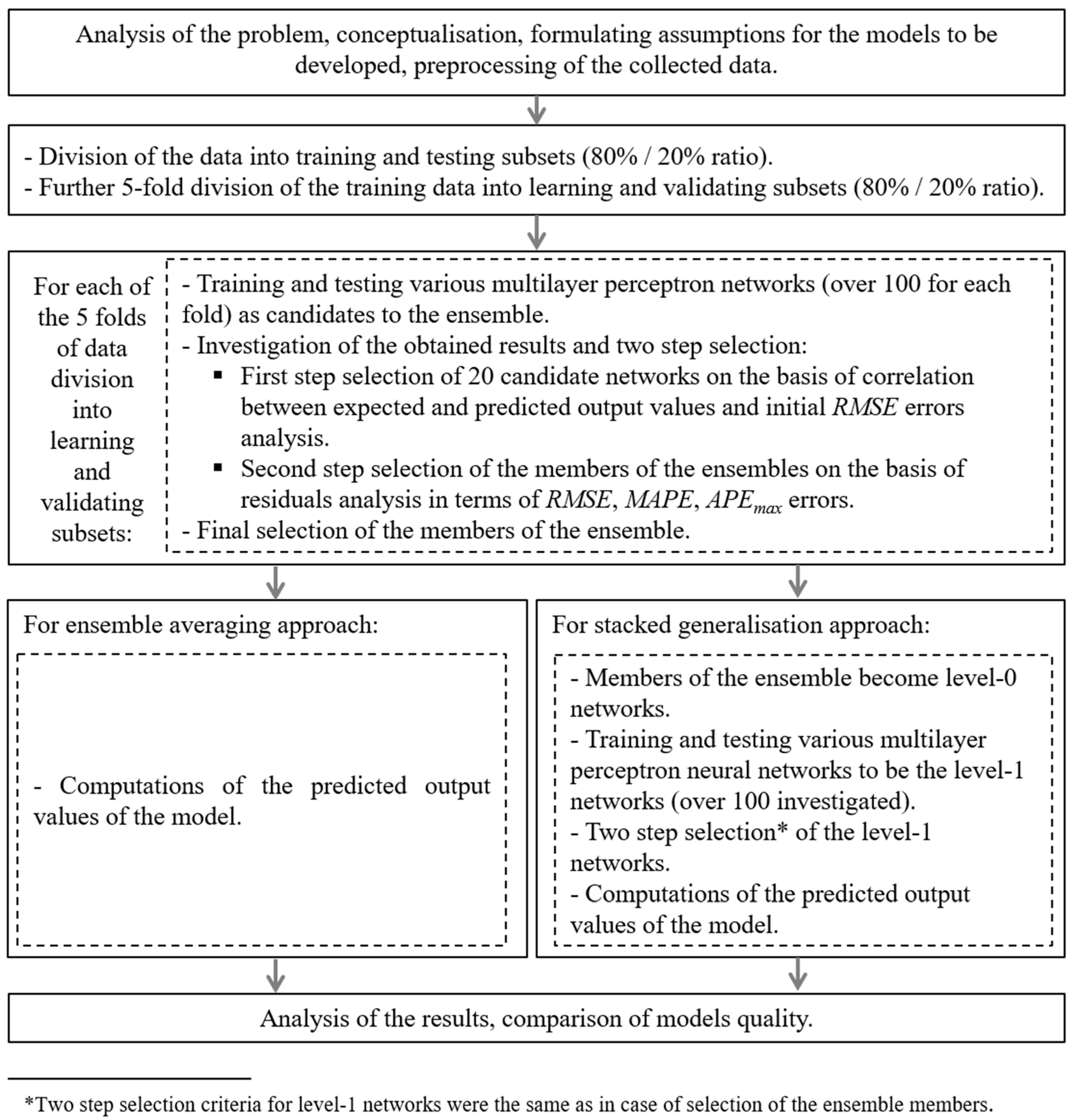
4.1. Models’ Development Strategy

The strategy of the model development included conducting multiple training and testing of a number of different types of single ANNs as candidates to become members of the ensemble, forming the ensemble, and then investigating the two approaches discussed earlier. The strategy is presented schematically in the chart in Figure 2 and then discussed in detail.

The whole set of collected data was divided into two main subsets used for training and testing purposes. The testing subset, later referred to as T, was selected carefully to be statistically representative for the whole data collection and included 20% of the samples from the whole set of collected data. The data belonging to this subset did not take part in the training of ANNs and was used for the purposes of examination of single ANNs, as well as the ensemble models built upon the ensemble averaging and stacked generalisation approaches. Samples belonging to the subset T play the role of new cases in prediction performance analysis as well.

The remaining data was used for training i.e., for supervised learning and validating of single ANNs candidates to become members of the ensemble. Later, these subsets are referred to as L and V, respectively, whilst the whole training subset is referred to as L&V. The strategy involved division of the remaining data in the relation L/V = 80%/20%, repeated five times, so the five folds of data were available for training purposes. Moreover, each of the samples belonging to the L&V subset took part in supervised learning in four folds and in validating in one fold, so the networks for each fold are trained with data which varies in terms of falling different samples either to the L or V subsets.

Another key assumption was to select one ANN for each of the folds of L and V subsets to become the member of the ensemble. The selection was made on the basis of two-step ANNs’ performance analysis and assessment within the sets of networks trained with the use of each fold of L and V subsets. The rationale for such assumption was not only to choose the best networks but also to minimise the risk that the prediction of the model is biased due to the sampling of the L and V subsets. The employed error function and criteria of the trained networks assessment are presented in

Table 4. Error function and models’ performance assessment criteria.

Description	Equation		Used As
sum-of-squares error function	$E_{sos}=\frac{1}{2}{\displaystyle \sum _{p\in L}}{\left(y^p-{\widehat{y}}^p\right)}^2$	(15)	error function
Pearson’s correlation coefficient	$R=\frac{cov\left(y,\widehat{y}\right)}{{\sigma }_y{\sigma }_{\widehat{y}}}$	(16)	criteria for general assessment of trained ANN’s quality (calculated for L, V, L&V, T subsets separately, cov(y,ŷ)—covariance between y and ŷ, σy—standard deviation for y, σŷ—standard deviation for ŷ)
root mean squared error	$RMSE=\sqrt{\frac{1}{c}{\displaystyle \sum _p}{\left(y^p-{\widehat{y}}^p\right)}^2}$	(17)	criteria for assessment of quality and performance of both trained ANNs and developed models based on ensembles (calculated for L, V, L&V, T subsets separately, c stands for L, V, L&V, T subsets cardinality, p stands for index of a training pattern)
mean absolute percentage error	$MAPE=\frac{100\%}{c}{\displaystyle \sum _p}\left|\frac{y^p-{\widehat{y}}^p}{y^p}\right|$	(18)
absolute percentage error	$AP{E}^p=\left|\frac{y^p-{\widehat{y}}^p}{y^p}\right|·100\%$	(19)
maximum of absolute percentage error	$AP{E}_{max}=max\left(\left|\frac{y^p-{\widehat{y}}^p}{y^p}\right|·100\%\right)$	(20)

. For the purposes of performance assessment and analysis of single ANNs, Pearson’s correlation coefficient (15) and error measures (16)–(20) were calculated for the L, V, L&V, and T subsets.

Selection of the ensemble members was preceded by an investigation of a number of various multilayer perceptron (MLP) ANNs with one hidden layer, whose structures included 11 neurons in the input layer, h neurons in the hidden layer, and 1 neuron in the output layer. The choice of the MLP networks relied on their applicability to regression problems (compare References [29,49]).

The networks varied in the number of neurons in the hidden layer (h ranged from 4 to 11), the types of employed activation functions—both in the neurons of the hidden and output layer (sigmoid, hyperbolic tangent, exponential, and linear function) and the initial weights of the neurons—at the beginning of the training process. The Broyden–Fletcher–Goldfarb–Shanno algorithm (BFGS) was used for training individual networks—the details about the algorithm can be found in the literature, e.g., Reference [47]. The choice of the training algorithm was dictated by its availability in the software that were used for neural simulations. As one of the three available algorithms, BFGS offered the fastest performance and best convergence of training and testing processes for the investigated problem. A variety of different combinations of employed activation functions and numbers of neurons in hidden layers that made, altogether, over 100 networks were trained for each of the five folds of L and V subsets.

The first step of selection included an assessment of correlation coefficient between the expected and predicted output and root mean squared error (RMSE) values. From the set networks, which fulfilled the conditions of R_L > 0.90, R_V > 0.90, R_L&V > 0.90, and R_T > 0.90, the authors initially selected 20 networks for which the differences between RMSE_L, RMSE_V, RMSE_L&V, and RMSE_T were the smallest.

The second step of the selection relied on a thorough review of the initially selected networks for each of the five folds of L and V subsets. The authors carried out a residual analysis, in terms of both measures presented in Table 4, and distributions, dispersions, and values of errors for the samples belonging to the training and testing subsets.

4.2. Results and Discussion

A review and comparison of the network’s performance, based on the methodical analysis, allowed for finally choosing five networks—one for each fold of L and V subsets. The five selected networks—later referred to as ANN1, ANN2, ANN3, ANN4, and ANN5—are presented in

Table 5. Details of the five networks selected to be the members of the ensemble.

ANN	Structure	Number of Neurons in the Hidden Layer	Hidden Layer Activation Function	Output Layer Activation Function	Number of Training Epochs
ANN1	MLP 11-10-1	10	hyperbolic tangent	hyperbolic tangent	146
ANN2	MLP 11-10-1	10	hyperbolic tangent	hyperbolic tangent	61
ANN3	MLP 11-6-1	6	exponential	linear	109
ANN4	MLP 11-8-1	8	hyperbolic tangent	exponential	67
ANN5	MLP 11-8-1	8	logistic	hyperbolic tangent	73

.

Table 6. Training results and performance of the selected networks.

ANN	R				RMSE				MAPE
	Training		Testing		Training		Testing		Training		Testing
	L	V	L&V	T	L	V	L&V	T	L	V	L&V	T
ANN1	0.9898	0.9662	0.9850	0.9731	0.0112	0.0206	0.01308	0.0181	6.0%	18.3%	8.4%	10.18%
ANN2	0.9861	0.9319	0.9761	0.9729	0.0131	0.0277	0.01643	0.0187	8.7%	14.5%	9.9%	10.19%
ANN3	0.9808	0.9645	0.9778	0.9804	0.0154	0.0198	0.01584	0.0159	10.4%	9.6%	11.3%	12.70%
ANN4	0.9868	0.9555	0.9737	0.9751	0.0128	0.0227	0.01482	0.0175	10.2%	13.1%	10.8%	13.69%
ANN5	0.9855	0.9278	0.9807	0.9881	0.0132	0.0296	0.01724	0.0123	11.1%	17.8%	12.5%	9.15%

presents the results of training and testing of the five selected networks acting separately. The results in the Table are given according to the criteria presented in Table 4. The results in Table 6 are satisfying, however one can easily see that there are some differences between the performances of the five networks.

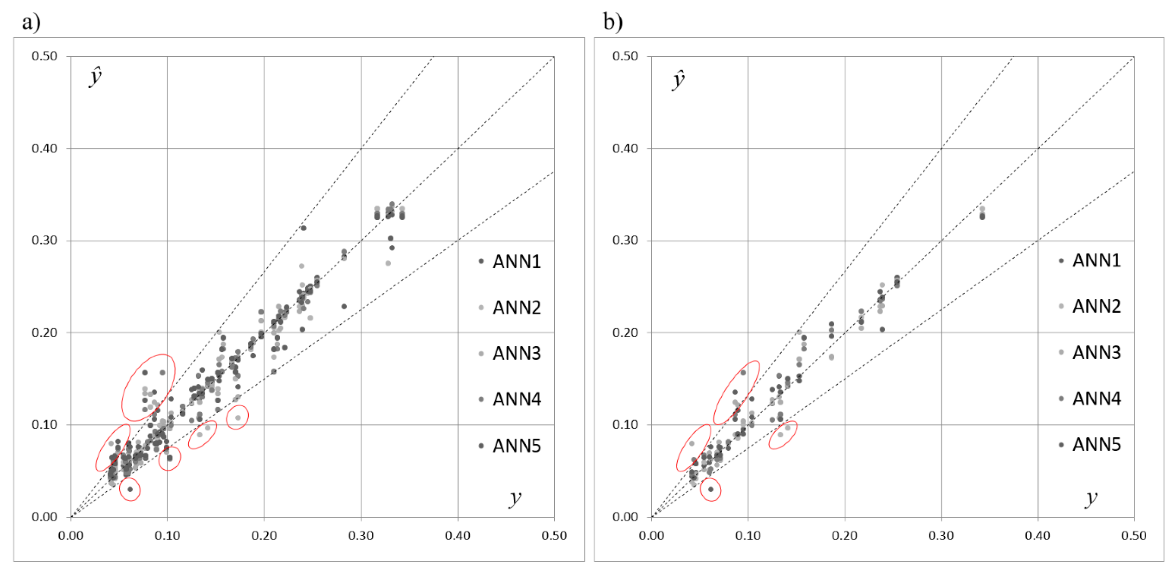
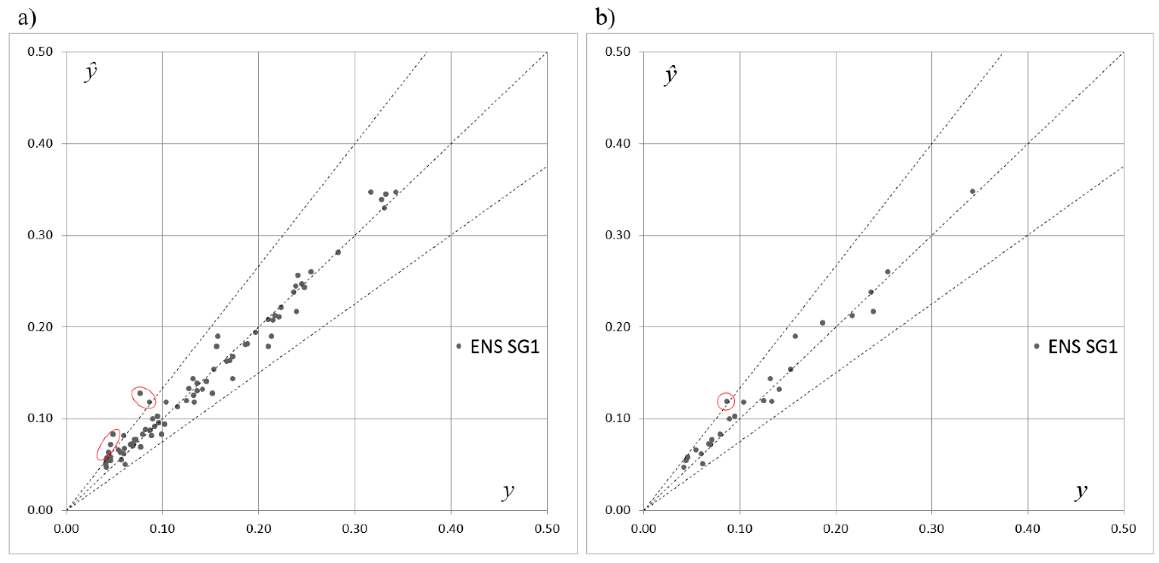
Figure 3 presents the scatterplot of the expected and predicted values of SOC_ind, points of coordinates (y^p, ŷ^p), for the training and testing subsets drawn for the five selected networks acting individually. One can see that, in terms of the criteria shown in Table 4 and according to the results presented in Table 5, the performance of the three networks acting individually was similar and the errors were comparable. However, Figure 3a,b and the analysis of the location and the distribution of the points in the graphs reveal that the predictions for will depended strongly on the choice of a single network acting separately. Although most of the points were distributed along the line of a perfect fit, some points (marked with the ellipses) were placed outside of the cone delimited by percentage errors equal to +25% and −25%.

Table 7. APE_max errors obtained for the five selected networks.

ANN	APEmax
	Training			Testing
	L	V	L&V	T
ANN1	65.9%	64.7%	65.9%	76.1%
ANN2	80.7%	45.2%	80.7%	33.4%
ANN3	73.2%	91.8%	91.8%	43.2%
ANN4	50.6%	64.4%	64.4%	70.1%
ANN5	53.3%	79.1%	79.1%	26.6%

presents the maximal values of absolute percentage errors (20) calculated for the five selected ANNs. The values in Table 7 reveal significant errors of predictions, which also justify employment of ensembles of neural networks in the problem.

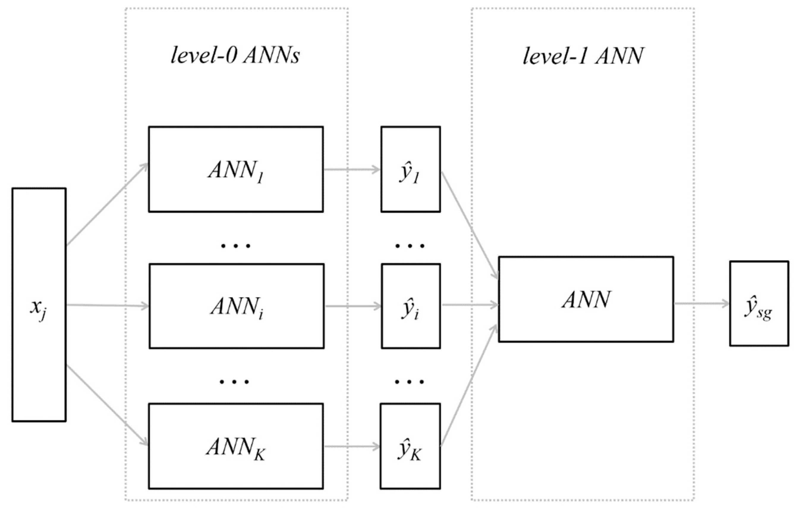
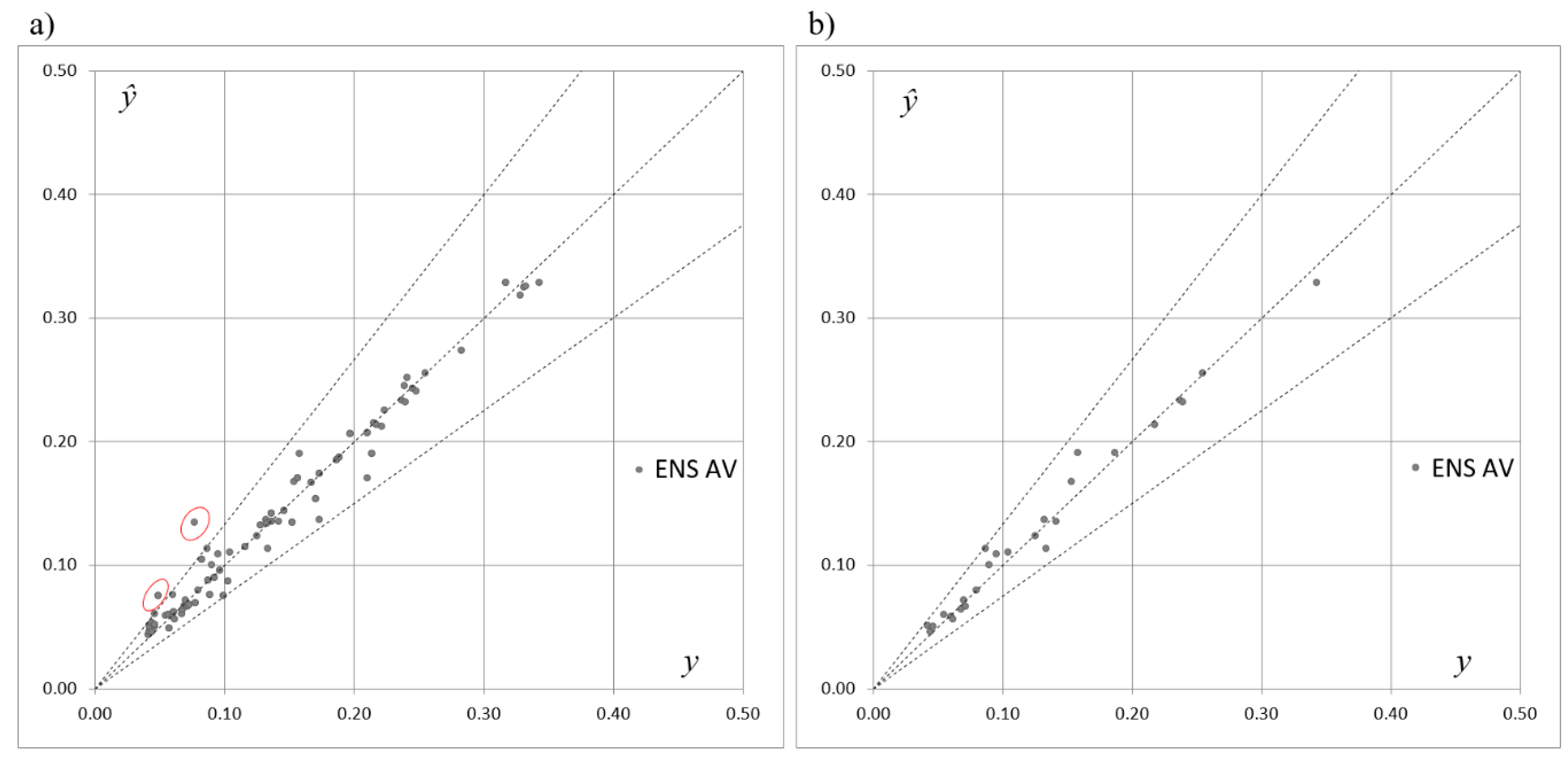
The five chosen networks were combined to form the ensemble. The rules presented earlier—Equations (10) and (11)—were employed for implementation of the ensemble averaging approach and the outputs of the model were computed as well as the errors and error measures. This model is later called ENS AV.

To complete the process of model development based on the stacked generalisation approach, the authors investigated a number of artificial neural-network candidates to become the level-1 networks. The investigated networks’ structures included five neurons in the input layer (as a consequence of the selection of five ensemble member networks), h neurons in the hidden layer, and one neuron in the output layer. The number of neurons in hidden layer h ranged from one to three, as the structure of the level-1 network was supposed to be simple (compare Section 2.2). The types of employed activation functions and training algorithm were the same as in the case of the training ensemble candidate networks (as presented previously in Section 3). Training patterns that included outputs of the five ensemble member networks as the inputs of level-1 networks, and the accompanying real-life values of SOC_ind as the expected outputs, were divided randomly for each investigated network into the learning and validating subset in the proportion L/V = 60%/40%. The investigated networks varied also in the initial weights of the neurons at the beginning of the training process. Altogether, around 100 networks were trained and examined. For the purposes of testing, the authors used the T subset, which was selected in the initial stage of the research (as presented previously in Section 3). The criteria of two-step selection of the level-1 networks were similar as in the case of ensemble candidate networks (as presented previously in Section 3). The final choice of two level-1 networks, namely MLP 5-2-1 and MLP 5-3-1, allowed for the introduction of two alternatively stacked generalisation-based models. The final choice of the two above-mentioned level-1 networks, and further discussion of two alternative models based on stacked generalisation, was due to the comparable quality of these models. These models are later called ENS SG1 and ENS SG2, respectively. The details of the selected level-1 networks are presented in

Table 8. Details of the two level-1 networks selected for the stacked generalisation-based models.

Model	Structure	Number of Neurons in the Hidden Layer	Hidden Layer Activation Function	Output Layer Activation Function	Number of Training Epochs
ENS SG1	MLP 5-2-1	2	exponential	linear	40
ENS SG2	MLP 5-3-1	3	exponential	exponential	51

.

All three proposed models based on the ensemble of networks, namely ENS AV, ENS SG1, and ENS SG2, were assessed in terms of performance and prediction quality. The overall results appear together in

Table 9. Performance measures for the three developed models based on the ensembles of networks.

Model	R		RMSE		MAPE		APEmax
	Training	Testing	Training	Testing	Training	Testing	Training	Testing
	L&V	T	L&V	T	L&V	T	L&V	T
ENS AV	0.9869	0.9899	0.0126	0.0112	8.3%	7.1%	42.6%	23.4%
ENS SG1	0.9853	0.9878	0.0135	0.0127	9.6%	9.2%	40.7%	26.7%
ENS SG2	0.9914	0.9922	0.0103	0.0098	7.3%	6.3%	23.2%	18.5%

. For the purposes of performance assessment and analysis of ensemble averaging and stacked generalisation-based models, Pearson’s correlation coefficient (16) and error measures (17), (18), (19), and (20) were calculated for L&V and T subsets.

When the values in Table 9 are collated with values in Table 5 and Table 6, the improvements in error measures can be seen easily. The performance of all three models based on the ensembles of networks is better when compared with the performance of the networks acting in isolation. The most evident improvement is achieved for APE_max.

Figure 4, Figure 5 and Figure 6 depict scatterplots of the expected and predicted values of SOC_ind for the ENS AV, ENS SG1, and ENS SG2 models. Figure 4, Figure 5 and Figure 6 present the points of coordinates (y^p, ${{\widehat{y}}^p}_{ens}$) for the training and testing subsets separately. When compared to Figure 3, these graphs show that combining the five selected ANNs allowed for the compensation of errors made by the ANNs acting in isolation in the case of the ENS AV as well as the ENS SG1 and ENS SG2 models. Although an improvement has been achieved in the case of all three introduced models, one can see that the best performance is provided by ENS SG2, where all of the points are distributed within the cone of acceptable errors. In the case of ENS AV and ENS SG1, there are single points located outside of the cone.

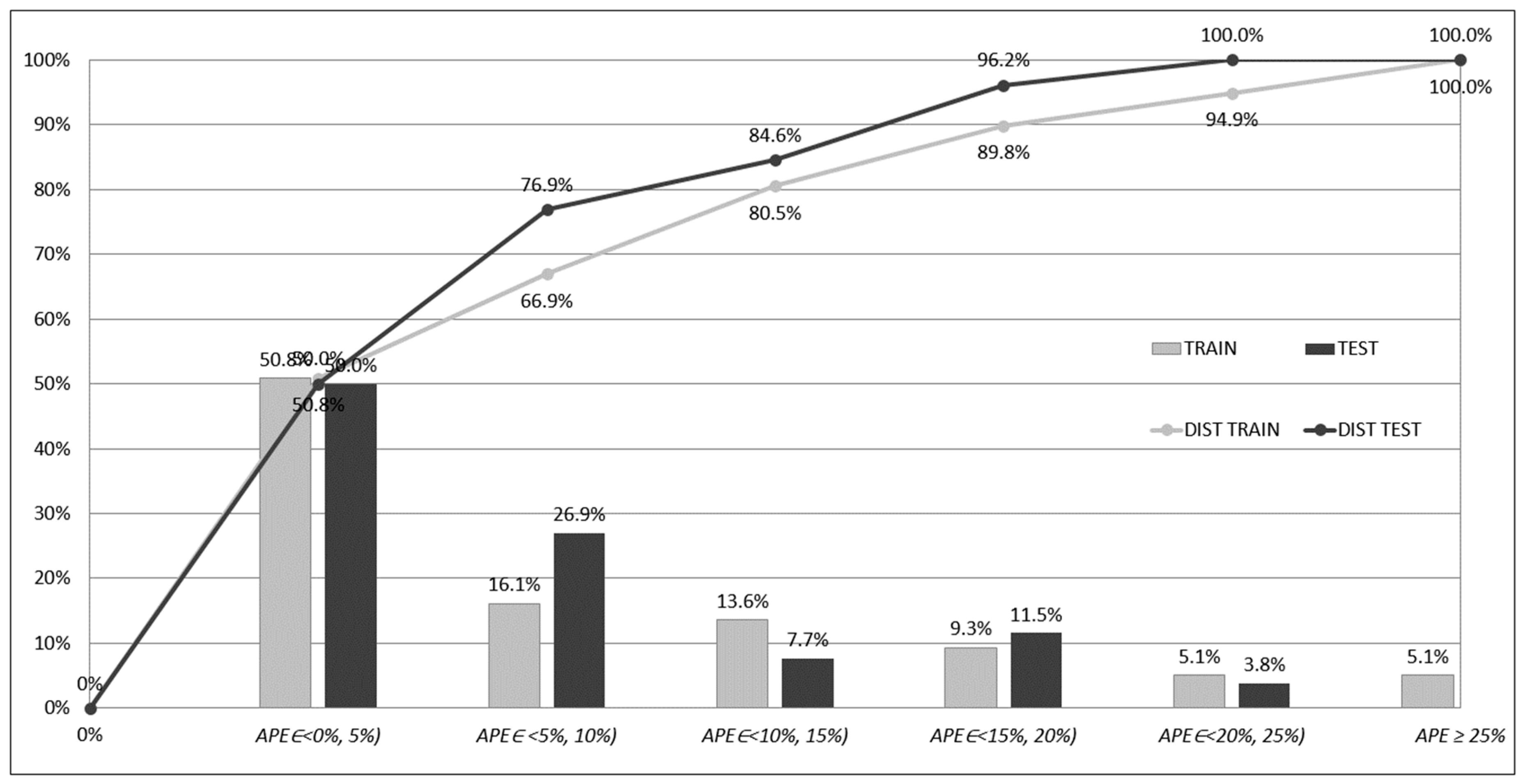
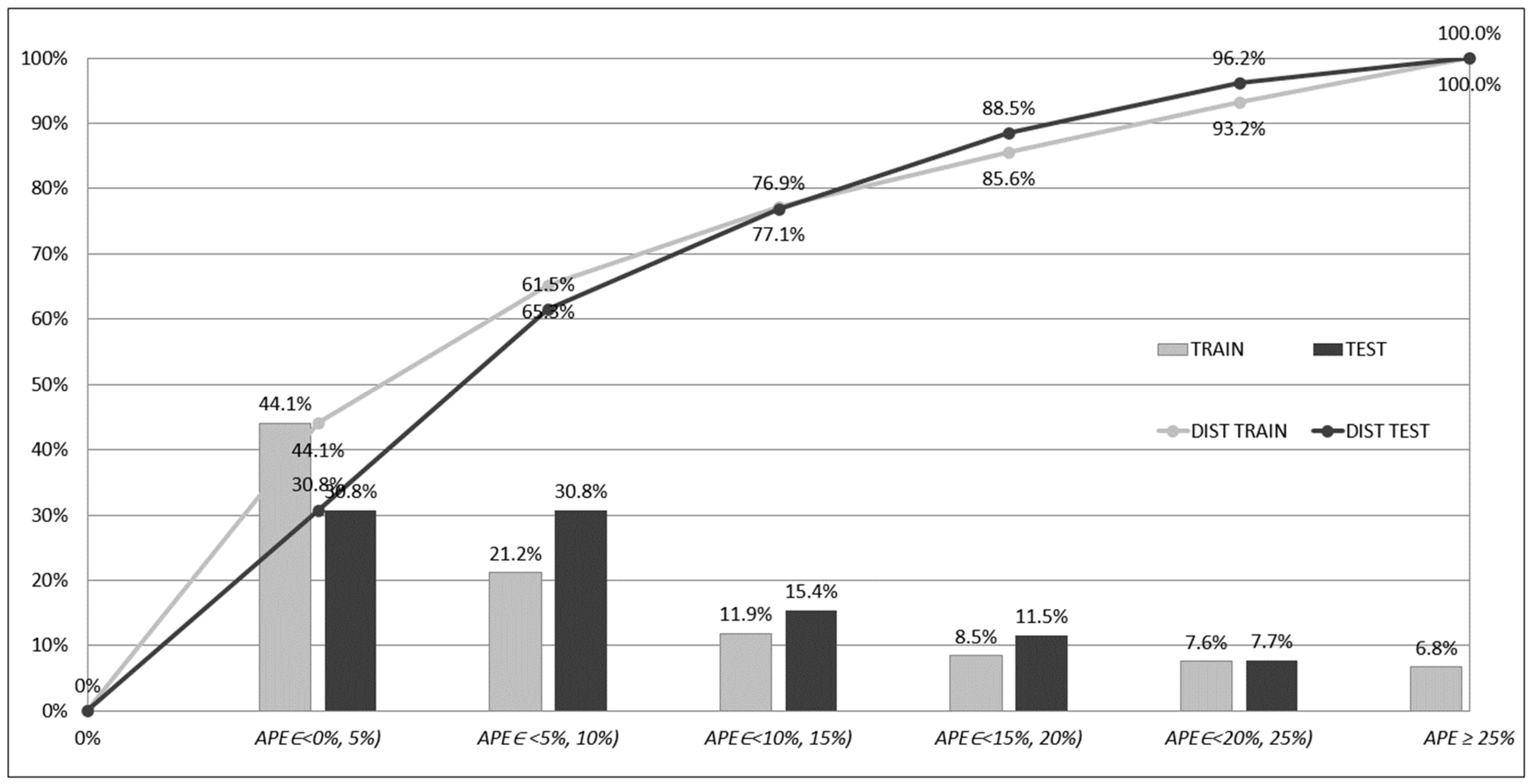
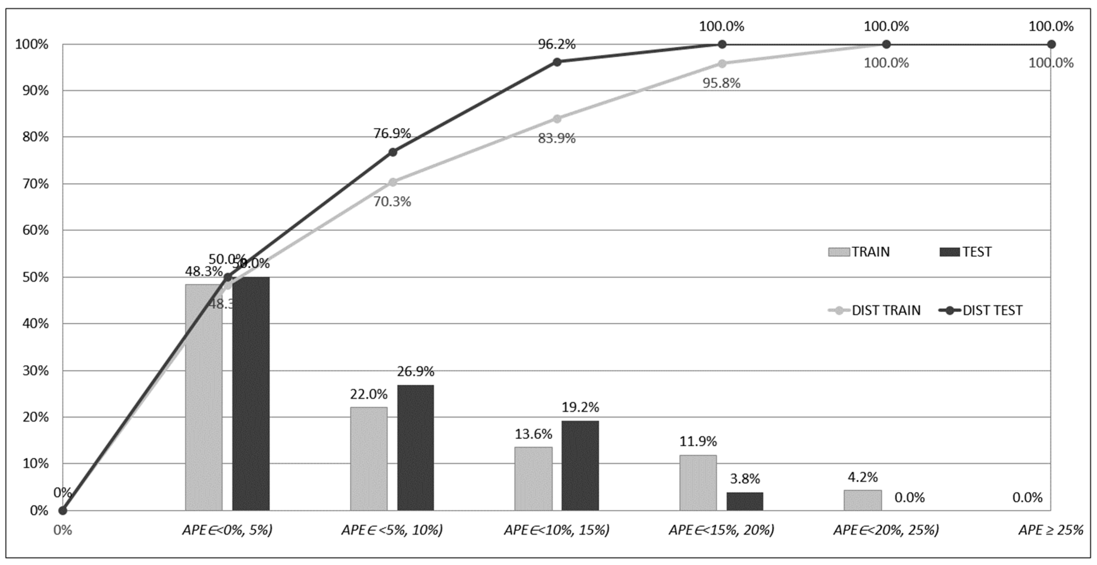
Figure 7, Figure 8 and Figure 9 depict frequencies and distributions of APE^p errors computed for the training and testing subsets for models based on ensembles of networks. The errors have been accumulated and counted in five intervals, whose ranges equalled 5%; one interval accumulated errors greater than 25%:

• interval 1: 0% ≤ APE^p < 5%,
• interval 2: 5% ≤ APE^p < 10%,
• interval 3: 10% ≤ APE^p < 15%,
• interval 4: 15% ≤ APE^p < 20%,
• interval 5: 20% ≤ APE^p < 25%,
• interval 6: APE^p ≥ 25%.

The columns in the Figure 7, Figure 8 and Figure 9 show the percentage frequencies of the errors that have fallen into one of the intervals. The polylines show the distribution of the errors (cumulative frequencies according to the accepted order of intervals). In Figure 7, Figure 8 and Figure 9, one can see that, in the case of the ENS AV and ENS SG1, only a few APE^p errors (19) are greater than 25%, and in the case of ENS SG2, none of them fall into this range. On the contrary, for networks acting separately, the significant number of errors is greater than 25%. These results can be explained through the analysis of the APE^p errors for the networks acting separately. For the networks acting separately (ANN1, ANN2, ANN3, ANN4, ANN5), many of the errors APE^p belonging to the interval 1 were relatively small and close to 0%. On the other hand, these small errors were accompanied by a significant number of errors APE^p ≥ 25%, and high values of APE_max (compare Table 7). In the case of the ensemble-based models, these errors have been compensated due to the ensemble averaging (ENS AV) or stacked generalisation (ENS SG1, ENS SG2).

The compensation resulted in the collection of most of the prediction errors in the first five intervals. One cost of this compensation is the decrease of the number of small errors, close to 0, in the first interval. The benefit of the compensation, however, is the improvement of the overall prediction performance and better knowledge generalisation. As mentioned previously, one can easily see that the best performance is offered by the ENS SG2 model as there were no errors APE^p ≥ 25%.

The analysis of the research results leads to the conclusion that the employment of only one of the five selected networks (as presented in Table 5) to support the prediction of SOC_ind would burden the predictions with the choice of a network—this is confirmed by the distribution of points that represent expected and predicted values (y^p, ${\widehat{y}}^p$) in Figure 3.

On the other hand, combining these five networks to form an ensemble compromises the strengths and weaknesses of the five ANNs—for some data, certain single-acting networks offered good predictions, whilst for others, there were weak predictions. Combining these networks into an ensemble allows for synergy. The decrease in APE_max, as well as more stable predictions, are the most beneficial from employment of the ensembles in the models. Furthermore, a risk of errors exceeding the critical level of 25%, in terms of percentage errors is reduced. These benefits have been achieved at some cost, mainly due to compensation of very small and very high errors offered by certain networks acting separately for certain training and testing patterns. However, the compensation of the errors from the ensemble-based models reduces the unwanted oversensitivity of the networks acting separately to certain training patterns.

5. Summary and Conclusions

The authors developed three original models based on ensembles of neural networks aimed at the prediction of site overhead cost index for construction projects. One of the models employed ensemble averaging and two of the models employed stacked generalisation. The developed models are capable of predicting the site overhead cost index with a satisfactory accuracy and, thus, supporting estimates of site overhead costs. In the light of the presented research, the general conclusion is that the employment of the ensemble of neural networks to the models proved to be superior over the approach based on the employment of a single neural network. Moreover, the effort—which is unavoidable in the training, verifying, and selecting number of networks of similar quality—is not wasted. In practical terms, the prediction using the ensemble averaging is simple—it needs an averaging of the outputs of networks belonging to the ensemble. On the other hand, stacked generalisation needs some additional computational effort that includes the training and selection of level-1 networks.

In the proposed approach, the authors employed an ensemble of neural networks to be the core of all three models. All of the proposed models consist of five different MLP networks, chosen from over 500 trained networks (over 100 networks were trained and investigated for each of five folds of training data). The five networks vary in their structure, employed activation functions, and initial conditions of training processes. The performance of the five chosen networks is comparable. However, the predictions made by the networks acting separately are burdened with the conditions of the training processes, sampling of learning and validating, and the specificity of each of the networks. Combining the five networks together leads to improvements in predictions due to compromising the strengths and weaknesses of the five networks. The prediction of the site overhead cost index using the ensemble-based models allowed for compensation of the errors made by the single networks. The predictions based on the three models for which the proposed ensemble is a core are more stable, and the risk of exceeding a critical range of errors is minimised.

The ensembles of neural networks proved their superiority over single neural networks acting in isolation. MAPE testing errors for the five networks acting in isolation ranged between 9.15% and 13.69%, whereas APE_max ranged between 26.6% and 76.1%. In the case of the proposed ensembles of networks, both MAPE and APE_max errors for testing were lower; values of MAPE ranged between 6.3% and 9.2%, whereas values of APE_max ranged between 18.5% and 23.4%. The quality of the ensemble-based model is also visible in the distribution of errors for each of them—more than 90% of the APE testing errors were smaller than 25%.

The three developed models, namely ENS AV (based on the ensemble averaging approach) and ENS SG1 and ENS SG2 (based on stacked generalisation approach), offer comparable prediction quality and performance, however the best results were achieved for ENS SG2. ENS SG2 is a two-level model that employs the five selected ANNs as the level-0 networks and simple ANN as a level-1 network.

The authors’ findings, justified by the analysis of the models’ performance, is that the developed models are capable of supporting estimation of site overhead costs in building construction projects. In the case of other types of constructions, e.g., bridges, roads, infrastructure, etc., the specificity of the projects must be taken into account and separate models must be developed.

Further research will include studies on the development of models, supporting the cost estimation process on different levels (for certain facilities, construction works, and cost components), that are based on the concept of ensembles of neural networks.

References

1. Leśniak, A.; Juszczyk, M. Prediction of site overhead costs with the use of artificial neural network based model. Arch. Civ. Mech. Eng. 2018, 18, 973–982. [Google Scholar] [CrossRef]
2. Gajzler, M.; Zima, K. Evaluation of Planned Construction Projects Using Fuzzy Logic. Int. J. Civ. Eng. 2017, 15, 641–652. [Google Scholar] [CrossRef]
3. Leśniak, A.; Plebankiewicz, E. Modeling the decision-making process concerning participation in construction bidding. J. Manag. Eng. 2013, 31, 04014032. [Google Scholar] [CrossRef]
4. Skorupka, D. Identification and initial risk assessment of construction projects in Poland. J. Manag. Eng. 2008, 24, 120–127. [Google Scholar] [CrossRef]
5. Tam, C.M.; Tong, T.K.; Chiu, G.C.; Fung, I.W. Non-structural fuzzy decision support system for evaluation of construction safety management system. Int. J. Proj. Manag. 2002, 20, 303–313. [Google Scholar] [CrossRef]
6. Hoła, B. Identification and evaluation of processes in a construction enterprise. Arch. Civ. Mech. Eng. 2015, 15, 419–426. [Google Scholar] [CrossRef]
7. Krzemiński, M. KASS v.2.2. Scheduling Software for Construction with Optimization Criteria Description. Acta Phys. Polon. A 2016, 309, 1439–1442. [Google Scholar] [CrossRef]
8. Chatterjee, K.; Zavadskas, E.K.; Tamošaitienė, J.; Adhikary, K.; Kar, S. A hybrid MCDM technique for risk management in construction projects. Symmetry 2018, 10, 46. [Google Scholar] [CrossRef]
9. Tamošaitienė, J.; Zavadskas, E.K.; Šileikaitė, I.; Turskis, Z. A novel hybrid MCDM approach for complicated supply chain management problems in construction. Procedia Eng. 2017, 172, 1137–1145. [Google Scholar] [CrossRef]
10. Zavadskas, E.K.; Antucheviciene, J.; Vilutiene, T.; Adeli, H. Sustainable decision-making in civil engineering, construction and building technology. Sustainability 2018, 10, 14. [Google Scholar] [CrossRef]
11. Anysz, H.; Zbiciak, A.; Ibadov, N. The Influence of Input Data Standardization Method on Prediction Accuracy of Artificial Neural Networks. Procedia Eng. 2016, 153, 66–70. [Google Scholar] [CrossRef] [Green Version]
12. Dikmen, S.U.; Sonmez, M. An Artificial Neural Networks Model for the Estimation of Formwork Labour. J. Civ. Eng. Manag. 2011, 17, 340–347. [Google Scholar] [CrossRef]
13. Schabowicz, K.; Hoła, B. Application of artificial neural networks in predicting earthmoving machinery effectiveness ratios. Arch. Civ. Mech. Eng. 2008, 8, 73–84. [Google Scholar] [CrossRef]
14. Yip, H.L.; Fan, H.; Chiang, Y.H. Predicting the maintenance cost of construction equipment: Comparison between general regression neural network and Box–Jenkins time series models. Autom. Constr. 2014, 38, 30–38. [Google Scholar] [CrossRef]
15. Leśniak, A. Supporting contractors’ bidding decision: RBF neural network application. AIP Conf. Proc. 2016, 1738, 200002. [Google Scholar] [CrossRef]
16. Wanous, M.; Boussabaine, H.A.; Lewis, J. A neural network bid/no bid model: The case for contractors in Syria. Constr. Manag. Econ. 2003, 21, 737–744. [Google Scholar] [CrossRef]
17. Ashraf, M.E. Classifying construction contractors using unsupervised-learning neural networks. J. Constr. Eng. Manag. 2006, 132, 1242–1253. [Google Scholar]
18. Mrówczyńska, M. Neural networks and neuro-fuzzy systems applied to the analysis of selected problems of geodesy. Comput. Assisted Mech. Eng. Sci. 2011, 18, 161–173. [Google Scholar]
19. Zavadskas, E.K.; Vilutienė, T.; Tamošaitienė, J. Harmonization of cyclical construction processes: A systematic review. Procedia Eng. 2017, 208, 190–202. [Google Scholar] [CrossRef]
20. Kapliński, O. Innovative solutions in construction industry. Review of 2016–2018 events and trends. Eng. Struct. Technol. 2018, 10, 27–33. [Google Scholar] [CrossRef]
21. Trost, S.M.; Oberlender, G.D. Predicting accuracy of early cost estimates using factor analysis and multivariate regression. J. Constr. Eng. Manag. 2003, 129, 198–204. [Google Scholar] [CrossRef]
22. Belniak, S.; Leśniak, A.; Plebankiewicz, E.; Zima, K. The influence of the building shape on the costs of its construction. J. Financ. Manag. Prop. Constr. 2013, 18, 90–102. [Google Scholar] [CrossRef]
23. Leśniak, A.; Zima, K. Cost calculation of construction projects including sustainability factors using the Case Based Reasoning (CBR) method. Sustainability 2018, 10, 1608. [Google Scholar] [CrossRef]
24. El Sawalhi, N.I. Modelling the parametric construction project cost estimate using fuzzy logic. Int. J. Emerg. Technol. Adv. Eng. 2012, 2, 2250–2459. [Google Scholar]
25. Kim, K.J.; Kim, K. Preliminary cost estimation model using case-based reasoning and genetic algorithms. J. Comput. Civ. Eng. 2010, 24, 499–505. [Google Scholar] [CrossRef]
26. Wilmot, C.G.; Mei, B. Neural network modeling of highway construction costs. J. Constr. Eng. Manag. 2005, 31, 765–771. [Google Scholar] [CrossRef]
27. Attala, M.; Hegazy, T. Predicting cost deviation in reconstruction projects: Artificial neural networks versus regression. J. Constr. Eng. Manag. 2003, 129, 405–411. [Google Scholar] [CrossRef]
28. El-Sawalhi, N.I.; Shehatto, O. Neural Network Model for Building Construction Projects Cost Estimating. J. Constr. Eng. Proj. Manag. 2014, 4, 9–16. [Google Scholar] [CrossRef]
29. Juszczyk, M. The challenges of nonparametric cost estimation of construction works with the use of artificial intelligence tools. Procedia Eng. 2018, 196, 415–422. [Google Scholar] [CrossRef]
30. Juszczyk, M. Application of committees of neural networks for conceptual cost estimation of residential buildings. AIP Conf. Proc. 2015, 1648, 600008. [Google Scholar] [CrossRef]
31. El-Sawy, I.Y.; Hosny, H.E.; Razek, M.A. A Neural Network Model for Construction Projects Site Overhead Cost Estimating in Egypt. Int. J. Comput. Sci. Issues 2011, 8, 273–283. [Google Scholar]
32. Juszczyk, M.; Leśniak, A. Site Overhead Cost Index Prediction Using RBF Neural Networks. In Proceedings of the 3rd International Conference on Economics and Management (ICEM 2016), Suzhou, China, 2–3 July 2016; DEStech Publications Inc.: Lancaster, CA, USA, 2016; pp. 381–386. [Google Scholar] [CrossRef]
33. Juszczyk, M. Implementation of the ANNs ensembles in macro-BIM cost estimates of buildings’ floor structural frames. AIP Conf. Proc. 2018, 1946, 020014. [Google Scholar]
34. Juszczyk, M.; Leśniak, A.; Zima, K. ANN Based Approach for Estimation of Construction Costs of Sports Fields. Complexity 2018, 2018, 7952434. [Google Scholar] [CrossRef]
35. Yazdani-Chamzini, A.; Zavadskas, E.K.; Antucheviciene, J.; Bausys, R. A Model for Shovel Capital Cost Estimation, Using a Hybrid Model of Multivariate Regression and Neural Networks. Symmetry 2017, 9, 298. [Google Scholar] [CrossRef]
36. Plebankiewicz, E.; Leśniak, A. Overhead costs and profit calculation by Polish contractors. Technol. Econ. Dev. Econ. 2013, 19, 141–161. [Google Scholar] [CrossRef]
37. Peurifoy, R.L.; Oberlender, G.D. Estimating Construction Costs, 4th ed.; McGraw Hill: New York, NY, USA, 1989. [Google Scholar]
38. Coombs, W.E.; Palmer, W.J. Construction Accounting and Financial Management, 4th ed.; McGraw Hill: New York, NY, USA, 1989. [Google Scholar]
39. Apanavičienė, R.; Daugėlienė, A. New Classification of Construction Companies: Overhead Costs Aspect. J. Civ. Eng. Manag. 2011, 17, 457–466. [Google Scholar] [CrossRef]
40. Chartered Institute of Building. Project Overheads, in Code of Estimating Practice, 7th ed.; Wiley-Blackwell: Oxford, UK, 2009. [Google Scholar]
41. Hegazy, T.; Moselhi, O. Elements of cost estimation: A survey in Canada and United States. Cost Eng. 1995, 37, 27–30. [Google Scholar]
42. Assaf, S.A.; Bubshait, A.A.; Atiyah, S.; Al-Shahri, M. The management of construction company overhead costs. Int. J. Proj. Manag. 2001, 19, 295–303. [Google Scholar] [CrossRef]
43. Brook, M. Preliminaries in Estimating and Tendering for Construction Work; Butterworth-Heinemann: Oxford, UK, 1998. [Google Scholar]
44. Cooke, B. Contract Planning and Contractual Procedures; Macmillan: Basingstoke, UK, 1981. [Google Scholar]
45. Assaf, S.A.; Bubshait, A.A.; Atiyah, S.; Al-Shahri, M. Project overhead costs in Saudi Arabia. Cost Eng. 1999, 41, 33–37. [Google Scholar]
46. Chan, C.T.W. The principal factors affecting construction project overhead expenses: An exploratory factor analysis approach. Constr. Manag. Econ. 2012, 30, 903–914. [Google Scholar] [CrossRef]
47. Bishop, P.C. Neural Networks for Pattern Recognition; Oxford University Press: Oxford, UK, 1995. [Google Scholar]
48. Haykin, S. Neural Networks: A Comprehensive Foundation; Macmillan Publishing: New York, NY, USA, 1994. [Google Scholar]
49. Rojas, R. Neural Networks: A Systematic Introduction; Springer Science & Business Media: New York, NY, USA, 2013. [Google Scholar]
50. Krogh, A.; Vedelsby, J. Neural network ensembles, cross validation, and active learning. In Advances in Neural Information Processing Systems, 7th ed.; Tesauro, G., Touretzky, D.S., Leen, T.K., Eds.; MIT Press: Cambridge, MA, USA, 1995; pp. 231–238. [Google Scholar]
Figure 1. General idea of stacked generalisation approach.
Symmetry 11 00411 g001
Figure 2. Scheme of the strategy of the models’ development.
Symmetry 11 00411 g002
Figure 3. Scatterplots of y and y ^ for the five selected neural networks acting separately: (a) scatterplot for samples belonging to the training subset, (b) scatterplot for samples belonging to the testing subset.
Symmetry 11 00411 g003
Figure 4. Scatterplot of y and y ^ e n s for the ensemble, ENS AV, performing ensemble averaging; (a) scatterplot for samples belonging to the training subset, (b) scatterplot for samples belonging to the testing subset.
Symmetry 11 00411 g004
Figure 5. Scatterplot of y and y ^ s g for the ensemble, ENS SG1; (a) scatterplot for samples belonging to the training subset, (b) scatterplot for samples belonging to the testing subset.
Symmetry 11 00411 g005
Figure 6. Scatterplot of y and y ^ s g for the ensemble, ENS SG2: (a) scatterplot for samples belonging to the training subset, (b) scatterplot for samples belonging to the testing subset.
Symmetry 11 00411 g006
Figure 7. Frequencies and distributions of absolute percentage errors for the ENS AV model computed for the training and testing subsets.
Symmetry 11 00411 g007
Figure 8. Frequencies and distributions of absolute percentage errors for the ENS SG1 model computed for the training and testing subsets.
Symmetry 11 00411 g008
Figure 9. Frequencies and distributions of absolute percentage errors for the ENS SG2 model computed for the training and testing subsets.
Symmetry 11 00411 g009