Abstract
As there are more and more available Web services with the same or similar functionalities but different Quality of Service (QoS), the challenge of QoS-aware service composition is to efficiently select appropriate component services to achieve maximum utility and meet the global QoS constraints with low time cost. In this paper, we propose a dynamic service selection approach based on adaptive global QoS constraints decomposition. Fuzzy logic technology and Cultural Genetic Algorithm are used to adaptively decompose global QoS constraints into near-optimal local constraints. According to the near-optimal local constraints, the optimal service is selected for each service class during the running time efficiently. Experimental results show that the proposed approach not only achieves the near-optimal solution, but also significantly reduces the computation time, and has good adaptability and scalability.
1. Introduction
Service-oriented architecture (SOA) is a modern paradigm to develop software systems that are often described as composite Web services [1]. Currently, composite Web services have been widely used in various areas, such as virtual enterprise, supply chain, accounting, finances, and e-Science. With the emergence of massive Web services, there are more and more candidate services that can provide the same or similar functionality. As a result, it is essential to consider Quality of Service (QoS) such as response time, price, availability, and so on [2,3]. In recent years, QoS-aware service composition has been widely studied [4,5].
Since Web services are invoked in a dynamic environment, the QoS attributes and user’s preferences are changing at runtime. In order to deal with the above runtime changes more efficiently and flexibly, dynamic service composition is proposed. It is described as a process containing a set of abstract services, and a concrete service is selected, bound, and invoked for each abstract service at runtime [6]. Moreover, users always put forward global QoS requirements, and as a result, it is demanded to select a concrete service for each abstract service that can satisfy global QoS constraints [7]. Service selection based on global QoS constraints is a combination optimization problem. The time complexity for the global optimization increases exponentially with the increasing of services or QoS attributes. Thus, it is a challenge to develop an efficient QoS-aware dynamic service selection approach that can maximize the utility and satisfy the global QoS constraints and user’s preferences as well.
Recently, researchers have carried out intensive studies on service selection based on global QoS constraints. The existing studies can be classified as optimization-based approaches and heuristic-based approaches. Optimization-based approaches aim at finding the optimization solution based on user’s QoS constraints [8,9]. These methods usually suffer from poor scalability due to the exponential time complexity. Heuristic-based approaches search for near-optimal solutions with a polynomial time complexity [10,11]. However, as these heuristic-based methods usually require a large number of global data and high cost of communication, they are not appropriate in distributed environments [12].
Currently, there are several heuristic-based methods based on global constraints decomposition [1,6,13,14]. In these methods, the value range of each QoS attribute of each service class is divided into a set of discrete values, which are called quality levels. The global QoS constraints are decomposed into local constraints for each service class by solving the optimal quality level scheme. Finally, local constraints are used to select local component service. These methods can achieve an approximate utility in dramatically reduced time and meet the global constraints as well. However, the above approaches do not discuss the number of quality levels, which is very important for service composition. Due to the constant number of quality levels, the above approaches are short of adaptability. As a result, the user’s preferences cannot be satisfied well. For example, some users need to find the composite service quickly instead of high quality; however, some users hope to get a trade-off between searching time and high quality.
To overcome the problems above, this paper proposes a dynamic service selection approach based on adaptive QoS constraints decomposition (AQCD). The main idea is to decompose global QoS constraints into local constraints, and according to the local constraints, select a component service for each service class independently. According to user’s preferences, utility function values, and time cost, we use fuzzy logic technology to automatically adjust the number of quality levels in order to generate the optimal quality level scheme. Finally, we use Cultural Genetic Algorithm (CGA) to solve the near-optimal global QoS constraints decomposition. In order to verify the effectiveness of our AQCD approach, extensive experiments were conducted on the real Web services data set QWS and the randomly generated data set RQWS. We compare the performances of AQCD, QCD, and the integer programming-based approach (WS-IP) by the running time and approximation ratio. Experimental results show that AQCD can efficiently solve the QoS-aware service composition problem with near-optimal solutions and low time cost. Further, it can fit well to user’s preferences and the increase in candidate services; that is to say, our approach has a good adaptability and scalability.
The remainder of this paper is organized as follows. Section 2 reviews related works. Section 3 briefly describes some basic concepts and formulates the service selection problem. Section 4 describes the process of dynamic service selection based on global QoS constraints decomposition. Section 5 proposes the adaptive adjustment approach based on fuzzy logic technology. Section 6 proposes the global QoS constraints decomposition approach based on CGA. Section 7 proposes the local service selection method. Section 8 presents experimental results. Finally, Section 9 concludes this paper.
2. Related Work
Web-service selection based on global QoS constraints considers the overall constraints provided by users, to find the optimal set of services. It is at the expense of high computation complexity to evaluate all the possible service compositions. To address this problem, a variety of approaches have been proposed. In References [8,9,15], QoS-aware service selection problem was modeled as a multidimensional multi-choice knapsack problem (MMKP). Integer programming methods [8,9,16] have been used to search for the optimal solution. The above approaches are very effective for small-scale problems. However, as the increasing of services, these approaches suffer from poor scalability because of the exponential time complexity.
To address the above problem, several bio-inspired algorithms [17] have been used to deal with QoS-aware service selection problem. There are three common bio-inspired algorithms used for service composition—genetic algorithm (GA) [18,19], ant colony optimization (ACO) algorithm [20,21], and particle swarm optimization (PSO) algorithm [22]. Furthermore, several researchers proposed improved bio-inspired algorithms to get better solutions with less time. References [11,23] provided a hybrid GA to solve the optimal service composition problem. Reference [24] proposed a variable length chromosome GA to deal with QoS-aware service selection. In Reference [25], QoS-aware service selection problem was modeled as a multi-objective optimization problem, and a multi-objective chaos ACO algorithm was proposed to solve it. Reference [26] proposed an immune optimization algorithm based on PSO and verified the better performances in aspects of the convergence rate, the searching ability, and the stability. Reference [10] proposed a cross-modified artificial bee colony algorithm to solve QoS-aware service selection. However, because of the requirement of global data visibility, it is difficult to apply these approaches in a distributed environment.
Recently, several QoS-aware service selection approaches based on global constraints decomposition have been proposed. From the viewpoint of computation time, the approach based on decomposition can be more appropriate and it can be applied in a distributed environment. The global constraints can be transformed to the local constraints through different approaches. Reference [27] discussed the constraints decomposition in the sequential, parallel, and condition structures, and then presented an approach for determining the local constraints in a general structure. Most works [1,6,13,14] divided the value range of each QoS attribute of each service class into discrete values, which were called quality levels. These approaches mapped global constraint into a set of quality levels. Finally, these quality levels were used as local constraints to select component service. However, all of the above approaches neglected the effect of the user’s preferences on the global constraints’ decomposition.
To overcome the above problem, this paper proposes a novel dynamic service selection approach based on adaptive global QoS constraints decomposition, in which the number of quality level is automatically adjusted.
3. Problem Formulation
In order to introduce the process of dynamic service selection based on global QoS constraints decomposition, this paper lists some basic concepts as below.
Definition 1.
Component service (): It is the basic unit in service composition, providing services to users.
Definition 2.
Service class
): A service class
denotes the
th abstract service of a composite Web service. It has m candidate services, which have the same functionality but differ in QoS attributes.
Definition 3.
QoS vector (): A QoS vector
contains
QoS attributes of service s.
Definition 4.
QoS aggregation for a composite service ():
contains
QoS attributes of a composite service. It can be calculated in terms of QoS values of component services and the composition structures.
Definition 5.
User preferences
:
represents user preferences, where
() is user’s preference for the
th QoS attributes.
, and
.
Definition 6.
Global QoS Constraints ():
is the set of user’s global QoS constraints, which contains
constraints and
() is a global constraint over
.
can be shown according to upper and/or lower bounds for the QoS aggregation value
.
3.1. QoS Aggregation for a Composite Service
There has been much research about service composition structures and QoS aggregation formulas. In Reference [27], the QoS attributes were divided into three different categories—additive attributes, multiplicative attributes, and max-operator attributes. There are four basic composition structures—sequential, parallel, conditional, and loop structures [27]. This paper only considers the sequential composition structure. Other composition structures can be converted to the sequential composition structure through the methods mentioned in Reference [27]. In this paper, we study five QoS attributes, including price, response time, availability, and throughput. We assume that a composite service is sequentially constructed by component services. The QoS aggregation formulas of five QoS attributes are as shown in Table 1.

Table 1.
Quality of Service (QoS) aggregation formulas for the sequential composition structure.
3.2. Utility Function
There are many candidate services with multiple QoS attributes in service composition. In order to calculate the QoS attributes of candidate services, we use the Simple Additive Weighting (SAW) approach [28] to map the QoS vector into a single real value.
Firstly, we should transform each QoS attribute into a real value between 0 and 1, which is called normalization. QoS attributes can be divided into two categories—negative attributes and positive attributes. For negative attributes (e.g., price), the lower the value, the higher the quality. On the contrary, for positive attributes (e.g., throughput), the higher the value, the higher the quality. Negative attributes can be easily converted into positive attributes by multiplying their values by −1. Therefore, this paper only considers the positive attributes. We define as the normalized value of the th QoS attribute of service and it can be calculated by Equation (1).
and are the maximum and minimum values of the th attribute of service class . is the value of the th attribute of candidate service .
Secondly, the utility function of component service () is shown as Equation (2), where represents the user’s preference assigned to the th QoS attribute.
The utility function of a composite service can be defined as Equation (3)
and are the maximum and the minimum values of the th attribute for . According to the formulas in Table 1, they can be calculated by aggregating the maximum and the minimum values of the th attribute of each service class.
4. Dynamic Service Selection Based on Global QoS Constraints Decomposition
The process of dynamic service composition in sequential composition structure is illustrated in Figure 1. There are service classes. Each service class has candidate services associated with QoS attributes. The concrete component service is selected and bounded from each corresponding abstract service class. The composite service needs to satisfy two conditions, as follows.
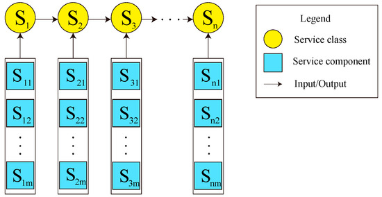
Figure 1.
Dynamic service composition in sequential composition structure.
(1) The utility function value of the composite service is maximum.
(2) The QoS aggregation for the composite service must satisfy the global QoS constraints, i.e., meets .
Recently, a number of service selection approaches based on global QoS constraints decomposition have been proposed, which can optimize the utility function value of the composite service while meeting the global constraints. As shown in Figure 2, these approaches basically have two components—global constraints decomposition and local service selection. Firstly, each global QoS constraint is decomposed into local constraints , where is the number of service classes. Secondly, the local constraints are used to select the optimal component service. The local constraints need to ensure that, as long as they are achieved, the global constraints are achieved. Furthermore, the local constraints should be general enough, in order to avoid ignoring any possible candidate service.
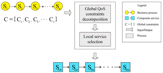
Figure 2.
Service selection based on global QoS decomposition.
5. Adaptive Adjustment Approach Based on Fuzzy Logic
In this section, we propose an adaptive adjustment approach, which uses fuzzy logic technology to adjust the number of quality levels automatically.
5.1. The Initialization of Quality Level
Quality levels are initialized for each QoS attribute of each service class by dividing the value range of each QoS attribute into discrete quality values as shown in Figure 3. represents the th QoS attribute value of the th candidate service of service class ; indicates the th quality level of the th QoS attribute of service class . It can be calculated as
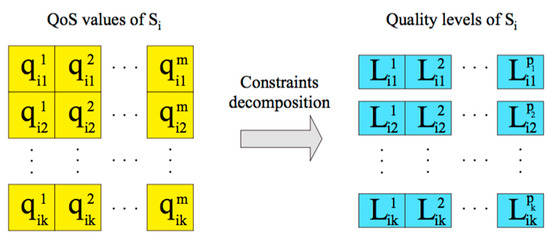
Figure 3.
The initialization of quality level.
, and is the number of quality levels of the th QoS attribute of service class . can computed as shown in Equation (5).
and are, respectively, the maximum and minimum quality value of service class for QoS attribute , and .
In this section, we exemplify the QoS constraints decomposition process by a composite service containing three sequential service classes with three QoS attributes. As shown in Table 2, each QoS attribute is associated to a weight and a constraint.
Table 2.
Global QoS constraints and weights.
We assume that the number of quality levels of each QoS attribute of each service class is 3. Figure 4 describes the procedure of the constraints’ decomposition. For service class , the global price constraint is divided into three local constraints , and .
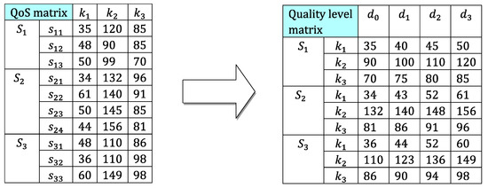
Figure 4.
The procedure of the constraints’ decomposition.
5.2. General Fuzzy Logic System
Fuzzy logic is an approximate reasoning technology based on multi-valued logic, which is suitable to deal with uncertainty [29]. It is able to support decision-making and evaluate uncertain parameters. In the existing researches [30,31,32,33], fuzzy logic technology has been used for service ranking in the process of service selection. In this paper, we propose an adaptive adjustment method for the number of quality level based on fuzzy logic (AAQL).
The general fuzzy logic system (FLS) includes four basic parts—fuzzification, fuzzy rule base, fuzzy inference, and defuzzification, as shown in Figure 5. The first step is fuzzification, in which crisp inputs are mapped into the fuzzy set. The fuzzy set can be defined by the membership function. Assuming that is a normal set, any function () that can map to [0,1], can determine a fuzzy set A. () is called the membership function. For any , () is the membership of , which describes the degree of belonging to . The next step is fuzzy inference, which determines what extent each rule in the fuzzy rule base applies to the current fuzzified inputs. IF–THEN rule is the common fuzzy rule to represent human knowledge in the general FLS. The IF part includes memberships of attributes of an individual, and the THEN part is a special concept called Rank. A fuzzy rule shows which composition of attributes a user is willing to accept to which degree, where attributes and degree of acceptance are vague [34]. A simple IF–THEN fuzzy rule can be:
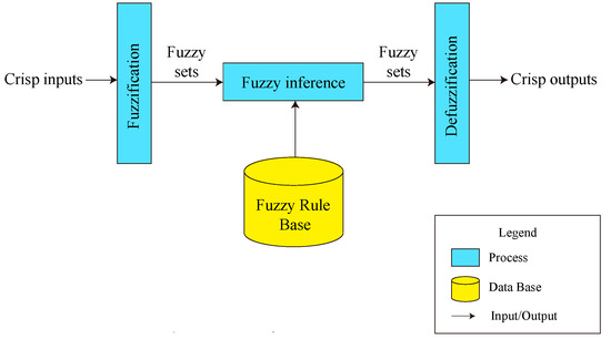
Figure 5.
General fuzzy logic system.
IF Price = Expensive and Time = Slow THEN Rank = Bad.
Finally, the fuzzified output is converted into a crisp output. This step is called “defuzzification”.
5.3. Adaptive Quality Level Based on Fuzzy Logic
AAQL can automatically adjust the number of quality levels according to user’s preferences [35], utility function values, and time cost. We assume that there are two input variables and one output variable. The input variables are the normalized number of quality levels of the th QoS attribute and the normalized function value of the quality levels . The output variable is , the change ratio of . and can be defined as below:
where or is the maximum or the minimum number of quality levels and is the current number of quality levels. or is the maximum or the minimum function value of the current quality levels. is the current function value of the quality levels, and it can be calculated as Equation (7).
is the user’s preference for the th attribute, and . can be dynamically obtained and normalized through the method in Reference [29]. Both and are the normalization value and and they can be calculated by Equation (8).
and are, respectively, the maximum and the minimum utility function values of the composite service under the current quality levels. is the current utility function value. and are, respectively, the maximum and the minimum time cost of the process of quality level initialization and quality level combination. is the current time cost.
Firstly, AAQL maps the input variables and into the fuzzy set. We assume that there are three fuzzy labels—L, M, and B, where L denotes “Little”, M denotes “Middle”, and B denotes “Big”. This paper uses the triangular and trapezoidal shapes to define membership functions of , , and , as shown in Figure 6.
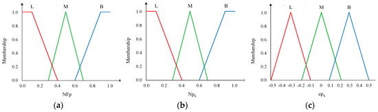
Figure 6.
The membership function of (a), (b), and (c).
Secondly, according to the fuzzy rules, AAQL uses the fuzzy inference to get the fuzzy output variable . The nine fuzzy rules of AAQL are as listed in Table 3, and the surface projection is shown as Figure 7. The basic fuzzy inference algorithm is Min–Max algorithm. However, the IF part consists of multiple attributes, which have different effects on the conclusion. For the Min algorithm, the conclusion is only determined by the attribute with the least membership. No matter how the membership of the other attributes change, as long as the minimum membership remains unchanged, the conclusion does not change. That is to say, Min–Max algorithm is insensitive to the changes of input facts. As a result, the common Min–Max algorithm is not suitable for AAQL. In this paper, we assign weights to and , respectively. Based on the weighted sum of and , we can infer the membership of the corresponding conclusion. Obviously, the weights are very important. At present, there is no definite method to get the exact weights. We designed a number of experiments by setting different user preferences and other parameters, and we conducted experiments to search for the optimal number of quality levels for each experiment. By summarizing the experimental results, we assign the weight of 0.7 and the weight of 0.3. Obviously, as the weights are set empirically, they are still not accurate. In our future work, we will improve the method for assigning the weights.
Table 3.
The fuzzy rules.
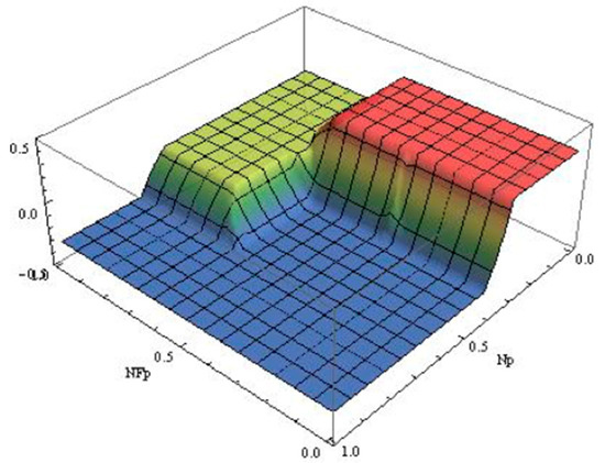
Figure 7.
The surface projection of fuzzy rules.
This paper adopts the center of gravity (COG) defuzzification method [36] to get the accurate and concrete value of . According to , the new number of quality levels can be adaptively adjusted as Equation (9), where is the new and is the original one.
For example, we assume that and . The calculation process of is as follows:
(1) Fuzzification of the input variables.
According to the membership functions in Figure 6, we can get the membership values of and , as shown in Table 4 and Table 5.
Table 4.
The membership values of .
Table 5.
The membership values of .
(2) Invoking the corresponding fuzzy rules.
When the fuzzy label of is L, the membership value is 0, and when the fuzzy label of is B, the membership value is 0. So, the fuzzy rules in Table 4, of which IF parts contain the fuzzy label of is L or the fuzzy label is B, are not be invoked. Finally, there are four rules invoked, which are listed in Table 6.
Table 6.
The activated rules.
Rule 1: The membership value of belonging to “M” is 0.35, and the membership value of belonging to “L” is 0.1, so the degree of Rule 1 can be calculated as: .
Rule 2: The membership value of belonging to “M” is 0.35, and the membership value of belonging to “M” is 0.35, so the degree of Rule 2 can be calculated as: .
Rule 3: The membership value of belonging to “B” is 0.1, and the membership value of belonging to “L” is 0.1, so the degree of Rule 3 can be calculated as: .
Rule 4: The membership value of belonging to “B” is 0.1, and the membership value of belonging to “M” is 0.35, so the degree of Rule 4 can be calculated as:
The conclusion of Rule 1 is the fuzzy label of is B, so the membership value of belonging to “B” is 0.275. For Rule 2, the fuzzy label of is L, so the membership value of belonging to “L” is 0.35. For Rule 3 and Rule 4, the fuzzy label is M, so the membership value of belonging to “M” is .
(3) Defuzzification of the output variable.
6. Global QoS Constraints Decomposition Based on CGA
6.1. Near-Optimal Quality Level Scheme
The nature of the optimal global QoS constraints decomposition is to search for an optimal quality level combination for each service class. Each service class has a number of QoS attributes and each QoS attribute has a set of quality levels, so there are many quality level schemes. It is a challenging problem to search for the optimal quality level scheme. It is a constrained multi-objected combinatorial optimization problem [37,38]. For large-scale searching space, in order to deal with this problem quickly, we use a novel evolution CGA by integrating Genetic Algorithm into the framework of Cultural Algorithm [1].
6.2. Cultural Genetic Algorithm
On account of parallelism and effective utilization of global information, GA is very suitable to solve combinatorial optimization problems. However, the prematurity phenomenon of GA is the biggest shortcoming. In order to assure the whole astringency, some approaches should be proposed to obtain the global optimal solution.
Cultural Algorithm (CA) is a new evolutionary algorithm to simulate the evolution of human society, proposed by Reynolds in 1994. As shown in Figure 8, CA is mainly composed of three parts—belief space, population space, and operation function. Belief space and population space can evolve at different speeds, which are relatively independent and interrelated. At the micro level, the population space simulates biological evolution and uses the evolutionary function PEvolve () to produce experiential knowledge. The evaluation function Evaluate () evaluates the information of the individuals in the population space, and then the useful information is passed to the belief space by function Accept (). Finally, the selection function Select () gives the optimal or approximate optimal solution. At the macro level, belief space uses Update () to receive, integrate, and preserve the empirical knowledge transmitted by the population space. Finally, the useful empirical knowledge is transferred to the population space by Influence (), so as to guide the evolution of individuals in the population space.
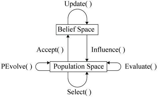
Figure 8.
The framework for Cultural Algorithm (CA).
To solve the constrained combinatorial optimization problem, it is the key problem how to transfer the constraints of the problem to the empirical knowledge and store it in the belief space. CA divides the searching space into several regions with different characteristics by using the constraint conditions.
We divide the searching space into smaller areas called cells. Some units are completely in the feasible domain, some units are completely in the infeasible domain, and the others are in both the feasible domain and infeasible domain. These units are the basic units that constitute the belief space of CA, called Belief Cells (BC). The belief space uses BC to represent and store the constraint conditions of the problem, in order to guide the evolution in the population space.
We take a constrained combinatorial optimization problem with two independent variables as an example. As shown in Figure 9, the solution space is a region in a two-dimensional plane. By several searching operations, a region that most likely produces excellent individuals is generated. We use a curve to represent the constraint boundary. The outer part of the curve is the feasible region and the inner part is the infeasible region. As shown in Figure 9b, the whole region is divided into smaller regions, which are BC. The BC belonging to the feasible region and infeasible region are represented by white and black squares, respectively, and the BC belonging to semi-feasible region are represented by gray squares. Constraint boundary and its internal constraint knowledge are saved as empirical knowledge to guide the population evolution in the population space, so that more individuals are generated in the feasible domain and semi-feasible domain, and the generation of individuals in the infeasible domain is restrained.
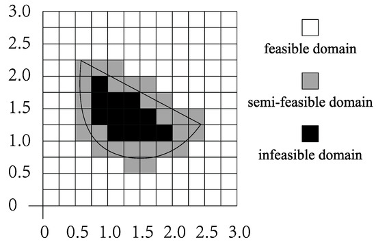
Figure 9.
Expression of constraints in area.
For an n-dimensional belief space containing m BC, its structure is defined as below:
N[] is the regional information set, and N[] represents the regional information of dimension j; C[] is the set of BC, and C[] is the th belief unit.
can be represented as follows:
is a closed interval that represents the value range of independent variables in the region of dimension j. , where is the upper limit value, and is the lower limit value. and are presented the evaluation function value of and , respectively.
can be represented as follows:
represents characteristics of the th belief cell, and the value set of is . 0 is feasible, 1 is not feasible, 2 is semi-feasible, and 3 is unknown. and are two counters that record the number of feasible and infeasible individuals in , respectively. is the weight of belief cell. The higher the credibility, the higher the weight of the belief cell. is the left-most angular position coordinate of the th belief unit and represents the size of the belief unit.
GA realizes population evolution by iterative operation through genetic operations such as selection, crossover, and mutation. This process is unguided and completely randomly. It ignores the important influence of feature information generated in the process of population evolution on solving problems. As a result, we take GA as the evolutionary algorithm of population space in CA and proposes knowledge guidance-based GA, namely Cultural Genetic Algorithm. CGA retains the selection and crossover operations of GA, and guides mutation operations with the empirical knowledge of the belief space, so as to effectively improve the convergence speed and the quality of results and reduce the computation time as well.
6.3. Global QoS Constraints Decomposition Algorithm Based on CGA
Suppose a composite service contains service classes and QoS attributes, and each QoS attribute is divided into constraint partitions. The flow chart of CGA is as shown in Figure 10. The optimal global QoS constraint decomposition algorithm based on CGA mainly includes two parts—the renewal of belief space and the evolution of population space.
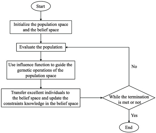
Figure 10.
The flow chart of Cultural Genetic Algorithm (CGA).
6.3.1. Belief Space Renewal
Belief space can be regarded as a hypercube composed of belief units in n-dimensional space. Through the functions Accept () and Update (), the belief space receives and integrates the empirical knowledge generated by the evolution of individuals in the population space, so as to constantly update the size of the hypercube.
The function Accept () sorts the individuals in the current population according to the size of their objective function values, and transfers the excellent individuals with large objective function values to the belief space. The number of individuals transferred to Accept () changes with the generations of population evolution. If the value of the overall objective function of the current population is greater than that of the previous generation, the number of individuals to be transferred will decrease. If it remains unchanged, the number of individuals to be transferred will remain unchanged. If it is less than that of the previous generation, the number of individuals to be transferred will increase. The number of excellent individuals transferred by the function Accept () in the paper is expressed by . The specific calculation formula is as follows:
represents the number of individuals in the population; is a parameter set up according to experience, generally 0.2. is the algebra of evolution; is a multiple of expansion. If the value of the overall objective function of the current population is larger than that of the population of the previous generation, or if the value of the overall objective function is constant, then h = 1. Otherwise, h = 2; that is, the number of selected individuals is increased. With the increase of population evolution algebra, when the population gradually converges to the optimal solution or approximate optimal solution, the computation amount and search time are gradually reduced, and the number of individuals is increased when the value of the objective function is not ideal.
According to the individual experience knowledge transferred by Accept (), Update () updates the belief space = ⟨, ⟩. Suppose that the th outstanding individual transferred in generation determines the lower limit of the independent variable value of , and the th outstanding individual determines the upper limit of the independent variable value of . Update by the following calculation formula:
Among them, the and represent the th independent variable of and in the th generation; and and , respectively, represent lower limit and upper limit of independent variables in the th generation of and , respectively, represent the utility function value of and .
6.3.2. Population Space Evolution
CGA takes GA as the evolutionary algorithm for population evolution in population space, which mainly includes the following key steps:
1. Encoding
The purpose of global QoS constraint decomposition is to find an appropriate constraint partition for each QoS attribute of each service class. A service composition scheme contains a number of service classes. There is a corresponding constraint partition set for each service class. Therefore, this paper designs a two-dimensional coding method to decompose a real, global QoS constraint. As shown in Figure 11, represents the th constraints division of the th QoS attribute of service class . Each column represents constraints division set of a service class.
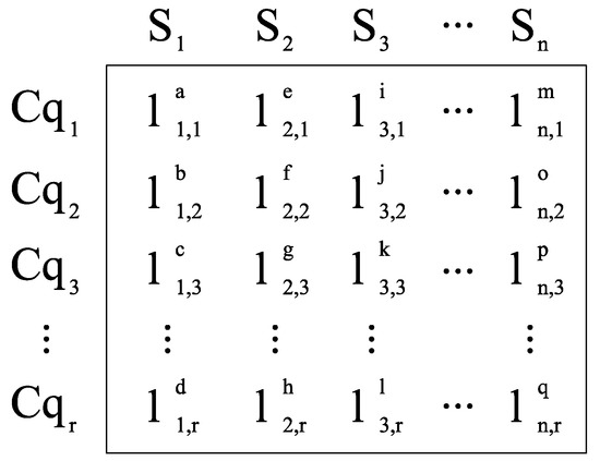
Figure 11.
The encoding method.
2. Evaluation Function
The evaluation function of CGA is to calculate the individual objective function value in the population. The specific calculation formula is as follows:
Among them, represents the th constraint division of the th QoS attributes of service class. represents if is selected or not, if selected or ; represents the user preference for the th QoS attribute. represents the constraint condition for attribute of composite service, and the evaluation function needs to meet the following conditions:
3. Selection Operation
According to the law of biological evolution, the larger the value of the objective function is, the greater the chance that individuals will be retained. That is to say, the probability of individuals being selected is directly proportional to the value of the objective function. The roulette selection method is adopted for individual selection operation. Let the population size be , and the probability of the th individual being selected is:
4. Crossover and Mutation Operation
After the selection operation, we select two individuals from the current population and perform the following operations:
Among them, and are two individuals of the th generation, and are new individuals, and is a random number. Choose one individual in the current population as parent individual. Its mutation operation is shown as follows, where is a new individual, is mutation step length, and is the variation direction.
5. Mutation Operation Based on Influence ()
New individuals generated by the basic mutation operation based on Equation (21) often violate the constraint conditions. In this paper, a mutation operation guided by the function Influence () in CA is used to generate new individuals. The specific calculation formula is divided into two situations:
- If the parent individual belongs to the feasible region or semi-feasible region, it continues mutating near the feasible region. Its computation formula is as follows:Among them, the is the th independent variable of the th generation individual ; is a artificial positive value; and , respectively, respect the upper limit and lower limit of the independent variable of th generation for ; represents a random value between 0 and 1.
- If the parent individual belongs to the infeasible region, we adopt the concept of the sliding window based on interval, move to four BC according to different probability. The computation formula is as follows:() is a migration function that moves the parent generation of an unfeasible domain to the selected target belief unit. represents that according to the probability of each BC , selecting the target BC by the roulette selection method for () invoking.When the th BC is selected, the formula of () is as follows:is a array, representing the most left position of the BC ; is a array, representing the size of BC in each dimension. is a array generated according to uniform distribution.
The pseudo code of the optimal global QoS constraints decomposition based on CGA is listed in Algorithm 1. For the scenario in Figure 4, we apply Algorithm 1 to obtain the near-optimal constraints decomposition scheme. The quality level matrix is the input set and the final result is shown in Table 7.
Table 7.
Optimal quality level combination.
| Algorithm 1 The optimal global QoS constraints decomposition based on CGA |
| Input: The initial quality partition set of each service class |
| Output: The optimal global QoS constraints decomposition scheme |
| 1. Initialize the population space |
| 2. Initialize the belief space |
| 3. Do |
| 4. Evaluate the individuals in the population space by Equation (15) |
| 7. Do selection operation by Equation (18) |
| 8. Do crossover operation by Equations (19) and (20) |
| 9. Do mutation operation by Equations (22) and (23) |
| 10. Calculate the number of excellent individuals transferred to the belief space Equation (10) |
| 11. Update the constraints knowledge in the belief space by Equation (11)–(14) |
| 10. While the termination condition is not met |
| 11. Return the optimal constraints decomposition scheme |
Therefore, the global QoS constraints in Table 2 are decomposed into local ones for each service class as shown in Table 8.
Table 8.
Local QoS constraints.
7. Local Service Selection
The local constraints are used to select component services from each service class in parallel. By the local constraints, we can reduce the number of the candidate services in each service class. In the reduced set of candidate services, the service with the biggest utility is selected as the final local component service. The utility function of component service can be defined as follows:
where is the th QoS attribute value of service , is the maximum value of the th QoS attribute values of service class , and is the weight of the th QoS attribute. Note that in Equation (25), we use the global utility function as the denominator, instead of the local utility function in Equation (1), so as to make the utility functions of the candidate services focus on global attributes.
According to the local constraints in Table 8, for service class , only the candidate service can meet the local constraints. Therefore, the candidate service is optimal to be bound to service class . Finally, the service combination (, , ) is generated as the optimal service composition scheme.
8. Experimental Evaluation
So as to evaluate the performance of the proposed approach (ACQD), we compare it with the integer programming-based approach (WS-IP) [16] and the QoS constraints decomposition approach based on CGA (QCD), in which the number of quality level is constant. Integer programming is widely applied for service selection [8,9,16].
Assuming that a service composition process in sequential structure contains six service classes, each service class has candidate services and varies from 100 to 1000. The data set consists of two parts: (1) QWS, a data set containing 2508 real Web services with 10 QoS attributes [39], and (2) RQWS, a data set artificially simulated and expanded according to QWS by Eclipse programming tool. In RQWS, the attributes and their ranges of services are the same as those of QWS. There are three global QoS attributes including price, response time, and availability. For RQWS, the QoS attribute values for each Web service are randomly generated, following Reference [40]. Table 9 shows the global QoS constraints and user’s QoS preferences in detail.
Table 9.
Global QoS constraints and user’s QoS preferences.
In our experiments, WS-IP was implemented by the open source system LpSolve (lp_solve version 5.5). For QCD and AQCD, we implemented them by Microsoft’s Visual C. Net and the rates of crossover and mutation operators were set as 0.80 and 0.10, respectively. All of the experiments were conducted on a PC with an Inter Core i5 (1.6 GHz) CPU and 4 GB RAM.
We evaluate the above approaches according to two metrics—running time and approximation ratio.
- Running time: the CPU time consumed by an algorithm.
- Approximation ratio: the ratio of the global utility achieved by an algorithm to the optimal utility. It can be computed as follows:
represents the utility function value and denotes the optimal utility function value. The optimal utility function value is generated by WS-IP. As a result, the approximation ratio of WS-IP is 1.
There are two experiments to evaluate the performance of AQCD. The first experiment evaluates the adaptability of AQCD compared with QCD and WS-IP, which consists of two parts. The first part evaluates how the number of quality levels affects QCD, in order to verify the importance of adjusting the number of quality levels. By analyzing the experimental results, the optimal number of quality number of quality levels is determined. The second part evaluates the performance of AQCD compared with QCD and WS-IP with different user’s preferences. Different user’s preferences or different numbers of candidate services per service class are set for every experiment. The average value of each experiment running 50 times is used to evaluate the method’s performance.
8.1. Evaluation of Adaptability
In this section, we firstly verify the importance of the number of quality levels to the performance of QCD. Then, we compare the performance of AQCD, QCD, and WS-IP with different user preferences to evaluate the adaptability of our approach AQCD.
8.1.1. The Number of Quality Level for QCD
The number of candidate services in each service class is set as 100 and the number of quality levels varies from 10 to 40. The running time and approximation ratio of QCD are recorded as shown in Figure 12 and Figure 13.
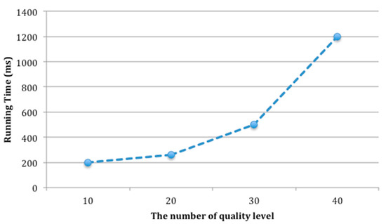
Figure 12.
Running time of QCD with different number of quality level.
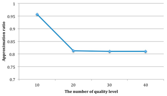
Figure 13.
Approximation ratio of QCD with different number of quality level.
As shown in Figure 12 and Figure 13, the number of quality levels has a prominent effect on the performance of service selection. In Figure 12, the running time increases rapidly with the increasing of the number of quality levels. Figure 13 indicates that when the number of quality level is 10, QCD can not only run fast, but also can obtain better solution. In other words, the optimal number of quality levels is 10, which is set for QCD.
8.1.2. Adaptability
So as to evaluate the adaptability of AQCD, we compare the performance of AQCD and other methods by changing the user’s preferences. We assume that there are 10 sets of user’s preferences. Among them, the user’s preferences in set 1 are set as shown in Table 9, and other sets are randomly generated. There are 100 candidate services in each service class and the number of quality levels for QCD is set as 10. The running time and approximation ratio of AQCD, QCD, and WS-IP with different user’s preferences are shown in Figure 14 and Figure 15.
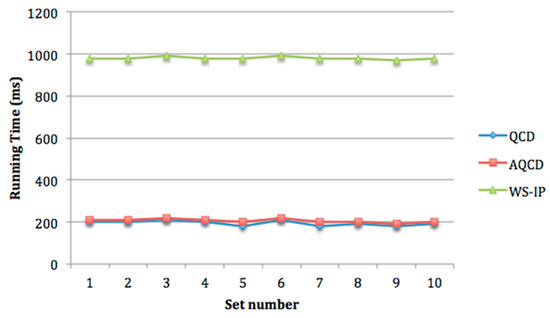
Figure 14.
Running time of QCD, AQCD, and WS-IP with different user’s preferences.
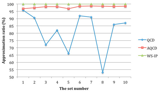
Figure 15.
Approximation ratio of AQCD, QCD, and WS-IP with different user’s preferences.
As shown in Figure 14, the running time of AQCD, QCD and WS-IP is almost stable with different user’s preference. The running time of AQCD is close to that of QCD all the time, and they are significantly shorter than WS-IP. Figure 15 shows that the approximation ratio of AQCD is better than QCD and close to the optimal method WS-IP. Furthermore, the approximation ratio of AQCD is stable with different user’s preferences. However, QCD suffers from user’s preferences. The approximation ratio of QCD changes with different user’s preferences.
8.2. Evaluation of Scalability
In order to evaluate the scalability of the proposed approach AQCD, we set the number of candidate services per service class from 100 to 1000. The experimental results of running time and approximate ration are shown in Figure 16 and Figure 17.
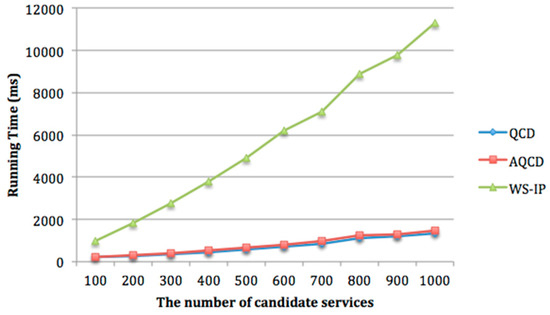
Figure 16.
Running time of QCD, AQCD, and WS-IP with different numbers of candidate services.
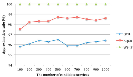
Figure 17.
Approximation ratio of QCD, AQCD, and WS-IP with different number of candidate services.
Figure 16 shows that with the increasing of candidate services, the running time of WS-IP is far more than that of AQCD and QCD. The running time of AQCD and QCD increases slowly. For a composite service composition with service classes, each service class contains candidate services and each service consists of QoS attribute. Each attribute can be divided into quality levels. In the worst case, the time complexity of WS-IP is . The running time of AQCD and QCD consists of two parts, the time of global constraints decomposition and local service selection. Among them, the local service selection is to select the component service for each service class in parallel. Its time complexity is . Therefore, the time complexity of AQCD and QCD mainly comes from the decomposition process of global constraints. The system needs to select one scheme from possible schemes. The time complexity is , which is independent of the number of candidate services . Therefore, when the number of quality levels is less than , the search space of AQCD and QCD is small. The running time of AQCD is slightly higher than QCD because it needs to adjust the number of quality level adaptively. However, this time is negligible. Figure 17 indicates that the approximation ratio of AQCD is higher than QCD and close to WS-IP. The approximation ratios of all the test cases are higher than 97%.
9. Conclusions
In this paper, a dynamic service selection approach based on adaptive global QoS constraints decomposition is proposed. We divided the global QoS constraints into local ones, by which the optimal component service for each service class is selected. We use fuzzy logic to automatically adjust the number of quality level considering the user’s preferences. In order to improve the efficiency of service selection, we use the Culture Genetic Algorithm to solve the near-optimal global constraints decomposition schema. Based on the real dataset QWS and the artificial generated dataset RQWS, we have evaluated the performance of the proposed approach AQCD in comparison with QCD and WS-IP. The experimental results show that the number of quality levels has a prominent effect on the performance of service selection. By adjusting the number of quality levels adaptively, the approximation ratio of AQCD can be stable with uncertain user’s preferences. With the increase in candidate services, AQCD can achieve near-optimal solutions with slowly increasing time, which is far less than that of WS-IP. In conclusion, our AQCD approach can achieve the near-optimal solution and significantly reduce the computation time. In addition, AQCD has good adaptability and scalability.
In our future work, we will increase the number of fuzzy sets and formulate more appropriate fuzzy rules in order to enhance the inference ability and manage complex situations; we will also apply the constraints decomposition approach to the problem of QoS-aware service composition in distributed environment where QoS values are maintained by a group of distributed QoS registries.
Author Contributions
Y.Y. conceived the research subject and wrote the paper. W.Z., X.Z., and H.Z. contributed to the revisions.
Funding
This research was funded by the National Natural Science Foundation of China (Grant No. 51479021, 51679025), Liaoning Provincial Natural Science Foundation of China (Grant No. 20170520196), the Fundamental Research Funds for the Central Universities (Grant No. 3132016308, 3132018197).
Conflicts of Interest
The authors declare no conflict of interest.
References
- Liu, Z.Z.; Xue, X.; Shen, J.Q.; Li, W.R. Web service dynamic composition based on decomposition of global QoS constraints. Int. J. Adv. Manuf. Technol. 2013, 69, 2247–2260. [Google Scholar] [CrossRef]
- Liu, C.Y.; Cao, J.; Wang, J. A Reliable and Efficient Distributed Service Composition Approach in Pervasive Environments. IEEE Trans. Mob. Comput. 2017, 16, 1231–1245. [Google Scholar] [CrossRef]
- Wang, P.W.; Liu, T.; Zhan, Y.; Du, X.Y. A Bayesian Nash Equilibrium of QoS-aware Web Service Composition. In Proceedings of the 24th IEEE International Conference on Web Services, Honolulu, HI, USA, 25–30 June 2017; pp. 676–683. [Google Scholar]
- Min, X.Y.; Xu, X.F.; Liu, Z.Z.; Chu, D.H.; Wang, J.Z. An approach to resource and QoS-aware service optimal composition in the big service and internet of things. IEEE Access 2018, 6, 39895–39906. [Google Scholar] [CrossRef]
- Bellavista, P.; Corradai, A.; Foschini, L.; Monti, S. Improved Adaptive and Survivability via Dynamic Service Composition of Ubiquitous Composition Middleware. IEEE Access 2018, 6, 33604–33620. [Google Scholar] [CrossRef]
- Ardagna, D.; Pernici, B. Adaptive service composition in flexible processes. IEEE Trans. Softw. Eng. 2007, 33, 369–384. [Google Scholar] [CrossRef]
- Siriweera, T.H.A.S.; Paik, I. QoS-Aware Rule-Based Traffic-Efficient Multiobjective Service Selection in Big Data Space. IEEE Access 2018, 6, 48797–448814. [Google Scholar] [CrossRef]
- Zeng, L.; Benatallah, B.; Kalagnanam, J.; Chang, H. QoS-aware middleware for web services composition. IEEE Trans. Softw. Eng. 2004, 19, 311–327. [Google Scholar] [CrossRef]
- Ding, Z.J.; Liu, J.J.; Sun, Y.Q.; Jiang, C.J.; Zhou, M.C. A Transaction and QoS-Aware Service Selection Approach Based on Genetic Algorithm. IEEE Trans. Syst. Man Cybern. Syst. 2017, 45, 1035–1046. [Google Scholar] [CrossRef]
- Huo, L.; Wang, Z.L. Service Composition Instantiation Based on Cross-Modified Artificial Bee Colony Algorithm. China Commun. 2016, 13, 233–244. [Google Scholar] [CrossRef]
- Yi, Q.; Wei, Z.; Chen, H.L. Improved adaptive immune genetic algorithm for optimal QoS-aware service composition selection in cloud manufacturing. Int. J. Adv. Manuf. Technol. 2018, 96, 4455–4465. [Google Scholar]
- Moustafa, A.; Zhang, M.J.; Bai, Q. Trustworthy Stigmergic Service Composition and Adaptation in Decentralized Environments. IEEE Trans. Serv. Comput. 2016, 9, 317–329. [Google Scholar] [CrossRef]
- Yong, Z.; Wei, L.; Luo, J.Z.; Zheng, X. A Novel Two-Phase Approach for QoS-Aware Service Composition Based on History Records. In Proceedings of the Fifth IEEE International Conference on Service-Oriented Computing and Applications (SOCA), Taipei, Taiwan, 17–19 December 2012; pp. 1–8. [Google Scholar]
- Yu, T.; Zhang, Y.; Lin, K.J. Efficient algorithms for Web services selection with end-to-end QoS constraints. ACM Trans. Web 2007, 1, 6–12. [Google Scholar] [CrossRef]
- Lu, W.; Wang, W.D.; Bao, E. FAQS: Fast Web Service Composition Algorithm Based on QoS-Aware Sampling. IEICE Trans. Fundam. Electron. Commun. Comput. Sci. 2016, E99A, 826–834. [Google Scholar] [CrossRef]
- Wang, L.J.; Shen, J. A Systematic Review of Bio-Inspired Service Concretization. IEEE Trans. Serv. Comput. 2017, 10, 493–505. [Google Scholar] [CrossRef]
- Tang, M.L.; Ai, L.F. A hybrid genetic algorithm for the optimal constrained web service selection problem in web service composition. In Proceedings of the World Congress on Computational Intelligence, Barcelona, Spain, 18–23 July 2010; pp. 1–8. [Google Scholar]
- Lecue, F.; Mehandjiev, N. Seeking Quality of Web Service Composition in a Semantic Dimension. IEEE Trans. Knowl. Data Eng. 2011, 23, 921–959. [Google Scholar] [CrossRef]
- Zheng, X.; Luo, J.; Song, A. Ant Colony System Based Algorithm for QoS-Aware Web Service Selection. In Proceedings of the 4th International Conference on Grid Service Engineering and Management (GSEM), Leipzig, Germany, 25–26 September 2007; pp. 39–50. [Google Scholar]
- Xia, Y.; Chen, J.; Meng, X. On the Dynamic Ant Colony Algorithm Optimization Based on Multi-Pheromones. In Proceedings of the Seventh IEEE ACIS International Conference on Computer and Information Science (ICIS ’08), Portland, OR, USA, 14–16 May 2008; pp. 619–635. [Google Scholar]
- Wang, W.; Sun, Q.; Zhao, X.; Yang, F. An Improved Particle Swarm Optimization Algorithm for QoS-Aware Web Service Selection in Service Oriented Communication. Int. J. Comput. Intell. Syst. 2012, 3, 18–19. [Google Scholar] [CrossRef]
- Cho, J.H.; Choi, J.H.; Ko, H.G.; Ko, I.Y. An Adaptive Quality Level Selection Method for Efficient QoS-aware Service Composition. In Proceedings of the IEEE 36th International Conference on Computer Software and Applications Workshops, Izmir, Turkey, 16–20 July 2012; pp. 20–25. [Google Scholar]
- Jiang, H.H.; Yang, X.H.; Yin, K.T.; Jerry, A. Multi-path QoS Aware Service Composition using Variable Length Chromosome Genetic Algorithm. Comput. Integr. Manuf. Syst. 2011, 10, 113–119. [Google Scholar] [CrossRef]
- Wang, L.; He, Y. A Web Service Composition Algorithm Based on Global QoS Optimizing with MOCACO. In Proceedings of the 2011 International Conference on Informatics, Cybernetics, and Computer Engineering (ICCE 2011), Melbourne, Australia, 19–20 November 2011; Volume 111, pp. 79–86. [Google Scholar]
- Zhao, X.; Song, B.; Huang, P.; Wen, Z.; Weng, J.; Fan, Y. An Improved Discrete Immune Optimization Algorithm Based on PSO for QoS-Driven Web Service Composition. Appl. Soft Comput. 2012, 12, 2208–2216. [Google Scholar] [CrossRef]
- Sun, S.A.; Zhao, J. A decomposition-based approach for service composition with global QoS guarantees. Inf. Sci. 2012, 199, 138–153. [Google Scholar] [CrossRef]
- Wang, S.G.; Sun, Q.B.; Yang, F.C. Web service dynamic selection by the decomposition of global QoS constraints. J. Softw. 2011, 22, 1426–1439. [Google Scholar] [CrossRef]
- Zhang, W.X.; Lang, Y.S. The Mathematical Basis of Genetic Algorithm (Version 2); Jiaotong University Press: Xi’an, China, 2004; pp. 66–72. [Google Scholar]
- Bakhshi, M.; Mardukhi, F. A Fuzzy-Based Approach for Selecting the Optimal Composition of Services According to User Preferences. In Proceedings of the 2nd International Conference on Computer and Automation Engineering (ICCAE), Singapore, 26–28 February 2010; pp. 129–135. [Google Scholar]
- Sharifara, P.; Yari, A.; Mansour, R.K. An Evolutionary Algorithmic based Web Service Composition with Quality of Service. In Proceedings of the 7th International Symposium on Telecommunications, Tehran, Iran, 9–11 September 2014; pp. 56–65. [Google Scholar]
- Kashyap, N.; Tyagi, K. Dynamic Composition of Web Services Based on Qos Parameters Using Fuzzy Logic. In Proceedings of the International Conference on Advances in Computer Engineering and Applications (ICACEA), Ghaziabad, India, 19–20 March 2015; pp. 308–782. [Google Scholar]
- Wu, Z.P.; Yuan, M. User-Preference-Based Service Selection Using Fuzzy Logic. In Proceedings of the 2010 International Conference on Network and Service Management, Niagara Falls, ON, Canada, 25–29 October 2010; pp. 321–345. [Google Scholar]
- Silvana, D.G.A.; Karim, D. Fuzzy Logic Based QoS Optimization Mechanism for Service Composition. In Proceedings of the 2013 IEEE Seventh International Symposium on Service-Oeiented System Engineering, Redwood City, CA, USA, 25–28 March 2013; pp. 182–191. [Google Scholar]
- Chuang, S.N.; Chan, A.T.S. Dynamic QoS adaptation for mobile middleware. IEEE Trans. Softw. Eng. 2008, 34, 738–752. [Google Scholar]
- Wang, H.B.; Zou, B.; Guo, G.B.; Yang, D.R.; Zhang, J. Integrating Trust with User Preference for Effective Web Service Composition. IEEE Trans. Serv. Comput. 2017, 10, 574–588. [Google Scholar] [CrossRef]
- Branson, J.S.; Lilly, J.H. Incorporation, Characterization, and Conversion of Negative Rules into Fuzzy Inference Systems. IEEE Trans. Fuzzy Syst. 2001, 9, 253–268. [Google Scholar] [CrossRef]
- Niu, S.; Zou, G.B.; Gan, Y.L.; Xiang, Y.; Zhang, B.F. Towards Uncertain QoS-aware Service Composition via Multi-objective Optimization. In Proceedings of the IEEE 24th International Conference on Web Services, Honolulu, HI, USA, 25–30 June 2017; pp. 894–897. [Google Scholar]
- Roy, R.; Dehuri, S.; Cho, S. A Novel Paricle Swarm Optimization Algorithm for Multi-Objective Combinational Optimization Problem. Int. J. Appl. Metaheurisitic Comput. 2011, 2, 41–57. [Google Scholar] [CrossRef]
- Al-Masri, E.; Mahmoud, Q.H. The QWS Dataset. Available online: http://www.uoguelph.ca/~qmahmoud/qws/index.html (accessed on 18 March 2019).
- Ren, L.F.; Wang, W.J.; Xu, H. A Reinforcement Learning Method for Constraint-Satisfied Services Composition. IEEE Trans. Serv. Comput. 2018, 7, 32–39. [Google Scholar] [CrossRef]
© 2019 by the authors. Licensee MDPI, Basel, Switzerland. This article is an open access article distributed under the terms and conditions of the Creative Commons Attribution (CC BY) license (http://creativecommons.org/licenses/by/4.0/).