Fuzzy Volterra Integro-Differential Equations Using General Linear Method

Abstract

In this paper, a fuzzy general linear method of order three for solving fuzzy Volterra integro-differential equations of second kind is proposed. The general linear method is operated using the both internal stages of Runge-Kutta method and multivalues of a multisteps method. The derivation of general linear method is based on the theory of B-series and rooted trees. Here, the fuzzy general linear method using the approach of generalized Hukuhara differentiability and combination of composite Simpson’s rules together with Lagrange interpolation polynomial is constructed for numerical solution of fuzzy volterra integro-differential equations. To illustrate the performance of the method, the numerical results are compared with some existing numerical methods.

1. Introduction

Fuzzy differential equations (FDEs) and fuzzy integral equations (FIEs) have been extensively studied in the past few years. They have appeared in many applications such as fuzzy matric spaces, population models, medicine, engineering problems, and others (see [1,2]). In the treatment of FDEs, one of the approaches was by using the definition of Hukuhara differentiability (see [3,4]). However, the Hukuhara differentiability experienced a disadvantage in its solutions. To overcome this, generalized Hukuhara differentiability was introduced by Bede and Gal in [5]. In the area of FIEs, the Rieman integral concept was proposed by Goetschel and Voxman in [6]. Another concept of integration is the Lebesgue concept by Kaleva in [7]. An early work in the numerical solutions of FDEs and FIEs is by Friedman et al. in [8]. Later, the area of interest in FIEs has been expanded into the fuzzy integro-differential equations (FIDEs). FIDEs take the form of both FDEs and FIEs. A particular class of FIDEs is known as fuzzy Volterra integro-differential equations (FVIDEs). The existence and uniqueness of FIDEs and FVIDEs solutions were investigated by Park and Jeong in [9], Hajighasemi et al. in [10], and Zeinali et al. in [11]. Mikaeilvand et al. in [12] presented the numerical examples of FVIDEs using the differential transform method. In [13], Allahviranloo et al. proposed a new technique to solve the FVIDEs using definition of generalized differentiability. Later, Allahviranloo et al. in [14] discussed the existence and uniqueness of second-order FVIDEs using the fuzzy kernel. Then Matinfar et al. in [15] solved the FVIDEs using the variational iteration method while Sahu and Saha Ray used Legendre wavelet method in [16].

In this work, we propose the numerical solutions of FVIDEs using the general linear method (GLM) introduced by Butcher in [17]. The GLM is a generalization of Runge-Kutta method (RK) and linear multistep method derived based on theory of B-series and definition of rooted trees. Recently, the GLM was studied for finding the numerical solutions of FDEs by Rabiei et al. in [18] and based on that, in this paper we develop the fuzzy third-order GLM together with suitable integration method to solve FVIDEs.

In Section 2, preliminaries on fuzzy numbers and theories are proposed. The concept of FVIDEs is discussed in Section 3. In Section 4, the general form of GLM is given followed by demonstration of the integration rules in Section 5. Then in Section 6, fuzzy version of the GLM combined with integration rules for FVIDE is developed while in Section 7, we derived the fuzzy RK method for FVIDEs using the same approaches used for GLM in Section 6. Section 8, some test problems are carried out to illustrate the efficiency of obtained method compared with a derived fuzzy RK method of order three in Section 7. Lastly, discussion and conclusion are presented in Section 9.

2. Preliminaries

In this section, some basic definitions on fuzzy numbers are given.

Definition 1

(see [19]). Consider a fuzzy subset of the real line $u:\mathbb{R}\to [0,1]$. Then u is a fuzzy number if it satisfies the following properties:

(i) 

u is normal, that is $\exists x_0\in \mathbb{R}$ with $u\left(x_0\right)=1$;

(ii) 

u is fuzzy convex, that is $u(tx+(1-t\left)y\right)\ge$ min $u\left(x\right),u\left(y\right)$, $\forall t\in [0,1],x,y\in \mathbb{R}$;

(iii) 

u is upper semicontinuous on $\mathbb{R}$, that is $\forall \epsilon >0\exists \delta >0$ such that $u\left(x\right)-u\left(x_0\right)<\epsilon ,|x-x_0|<\delta$;

(iv) 

u is compactly supported, that is $cl\{x\in \mathbb{R};u(x)>0\}$ is compact, where $cl\left(A\right)$ denotes the closure of the set A.

Then ${\mathbb{R}}_F$ is called the space of fuzzy numbers.

Definition 2

(see [19]). For $0<r\le 1$, we have

$${\left[u\right]}^r=\{x\in \mathbb{R};u\left(x\right)\ge r\},$$

and

$${\left[u\right]}^0=cl\{x\in \mathbb{R};u\left(x\right)>r\}\}.$$

Then the ${\left[u\right]}^r$ denotes the r-level set of the fuzzy number u. The 1-level will refer to the core while the 0-level refers to the support of the fuzzy number.

Proposition 1

(see [19]). A fuzzy number u is a pair $u=(u^{-},u^{+})$ of functions $u^{-},u^{+}:[0,1]\to \mathbb{R}$, implying the end points of r-level set, following the conditions:

(i) 

$u_r^{-}\in \mathbb{R}$ is a bounded nondecreasing left-continuous function $\forall r\in [0,1]$ and right-continuous for $r=0$;

(ii) 

$u_r^{+}\in \mathbb{R}$ is a bounded nonincreasing left-continuous function $\forall r\in [0,1]$ and right-continuous for $r=0$;

(iii) 

$u_r^{-}\le u_r^{+}$ for $r=1$, which implies $u_r^{-}\le u_r^{+},\forall r\in [0,1].$

Definition 3

(see [19]). Let $u,v\in {\mathbb{R}}_F$, the distance $D(u,v)$ between two fuzzy intervals is defined by

$$D_{\infty }(u,v)=\underset{r\in [0,1]}{sup}max\left\{\right|u_r^{-}-v_r^{-}|,|u_r^{+}-v_r^{+}\left|\right\}.$$

Then $D_{\infty }(u,v)$ is the Hausdorff distance between fuzzy numbers.

Proposition 2

(see [19]). It is said that $D_{\infty }(u,v)$ is a metric space in ${\mathbb{R}}_F$ and the following properties hold:

(i) 

$D_{\infty }(u+w,v+w))=D_{\infty }(u,v),\forall u,v,w\in {\mathbb{R}}_F;$

(ii) 

$D_{\infty }(k·u,k·v)=\left|k\right|D_{\infty }(u,v),\forall u,v\in {\mathbb{R}}_F,\forall k\in \mathbb{R};$

(iii) 

$D_{\infty }(u+v,w+e)\le D_{\infty }(u,w)+D_{\infty }(v,e),\forall u,v,w,e\in {\mathbb{R}}_F.$

Definition 4.

A function $f:\mathbb{R}\to {\mathbb{R}}_{\mathcal{F}}$ is said to be fuzzy continuous function if f exists for any fixed arbitrary $g_0\in \mathbb{R}$ and $\epsilon >0,\delta >0$ such that $|g-g_0|<\delta ⟹D[f\left(g\right),f\left(g_0\right)]<\epsilon$.

Definition 5.

Let $x,y\in {\mathbb{R}}_{\mathcal{F}}$. If there exists $z\in {\mathbb{R}}_{\mathcal{F}}$ such that $x=y\oplus z$, then z is called the Hukuhara difference (H-difference) of x and y and it is denoted by $x\ominus y$. (Please note that, $x\ominus y\ne x+(-y)$).

Definition 6

(see [5]). Let $f:(a,b)\to {\mathbb{R}}_F$ and $x_0\in (a,b)$. f is known as strongly generalized differentiable at $x_0$, if there exists an element $f^{\prime }\left(x_0\right)\in {\mathbb{R}}_F$ such that

(i) 

for all $h>0$ sufficiently small, $\exists f(x_0+h)\ominus f\left(x_0\right),f\left(x_0\right)\ominus f(x_0-h)$ and the limits in metric D

$$\underset{h\searrow 0}{lim}\frac{f(x_0+h)\ominus f\left(x_0\right)}{h}=\underset{h\searrow 0}{lim}\frac{f\left(x_0\right)\ominus f(x_0-h)}{h}=f^{\prime }\left(x_0\right),$$

(1)

is type-$\left(i\right)$-differentiability on $(a,b)$,

(ii) 

for all $h>0$ sufficiently small, $\exists f\left(x_0\right)\ominus f(x_0+h),f(x_0-h)\ominus f\left(x_0\right)$ and the limits in metric D

$$\underset{h\searrow 0}{lim}\frac{f\left(x_0\right)\ominus f(x_0+h)}{(-h)}=\underset{h\searrow 0}{lim}\frac{f(x_0-h)\ominus f\left(x_0\right)}{(-h)}=f^{\prime }\left(x_0\right).$$

(2)

is type-$\left(ii\right)$-differentiability on $(a,b)$,

Theorem 1

(see [20]). Let $F:T\to {\mathbb{R}}_F$ be a function and denote ${\left[F\left(t\right)\right]}_r=[f_r\left(t\right),g_r\left(t\right)]$, for each $r\in [0,1]$. Then

(i) 

If F is differentiable in the first form (1), then $f_r$ and $g_r$ are differentiable functions and ${\left[F^{\prime }\left(t\right)\right]}_r=[f_r^{\prime }\left(t\right),g_r^{\prime }\left(t\right)]$,

(ii) 

If F is differentiable in the second form (2), then $f_r$ and $g_r$ are differentiable functions and ${\left[F^{\prime }\left(t\right)\right]}_r=[g_r^{\prime }\left(t\right),f_r^{\prime }\left(t\right)]$.

Definition 7

(see [15]). Let $f:[a,b]\to {\mathbb{R}}_F$, for each partition $P=\{t_0,t_1,\cdots ,t_n\}$ of $[a,b]$ and for arbitrary ${\xi }_i\in [t_i-1,t_i],1\le i\le n$, and suppose

$$\begin{array}{cc}\hfill {\mathit{R}}_p& =\sum _{i=1}^n\left({\xi }_i\right)(t_i-t_{i-1}),\hfill \\ \hfill \Delta :& =max\left\{\right|t_i-t_{i-1}|,1\le i\le n\}.\hfill \end{array}$$

The integration of $f\left(t\right)$ over $[a,b]$ is

$${\int }_a^{b}f\left(t\right)dt=\underset{\Delta \to 0}{lim}{\mathit{R}}_p,$$

given that in metric D, the limit exists. The definite integral of fuzzy function $f\left(t\right)$ exists, if $f\left(t\right)$ is continuous function in metric D, and

$$\begin{array}{cc}\hfill {\left({\int }_a^{b}f\left(t\right)dt\right)}_r^{-}& ={\int }_a^b{f}_r^{-}\left(t\right)dt,\hfill \\ \hfill {\left({\int }_a^{b}f\left(t\right)dt\right)}_r^{+}& ={\int }_a^b{f}_r^{+}\left(t\right)dt.\hfill \end{array}$$

3. Fuzzy Volterra Integro-Differential Equations

Consider the first order fuzzy initial value problems of second kind FVIDEs given by

$$y^{\prime }\left(t\right)=f(t,y)+{\int }_0^{x}K(t,s)y\left(s\right)ds,y\left(t_0\right)=y_0\in {\mathbb{R}}_F,$$

(3)

and in short notation is given as

$$y^{\prime }\left(t\right)=f\left(t,y,{\int }_0^{x}K(t,s)y\left(s\right)ds\right),y\left(t_0\right)=y_0\in {\mathbb{R}}_F,$$

(4)

where function $f:\mathbb{R}\times {\mathbb{R}}_F\to {\mathbb{R}}_F$, crisp function $K(t,s)$ are continuous and $y_0$ is a fuzzy number.

Using Theorem 1, and extending the characterization theorem in [19], FVIDE given in (4) for type (i)-differentiability is equivalent to the following system of ODEs:

$$\left\{\begin{array}{c}{\left(y_r^{-}\right)}^{\prime }\left(t\right)=f_r^{-}(t,y_r^{-},y_r^{+})+{\int }_0^t{K}^{-}(t,s)y\left(s\right)ds=F(t,y_r^{-},y_r^{+},{\int }_0^t{K}^{-}(t,s)y\left(s\right)ds),\hfill \\ {\left(y_r^{+}\right)}^{\prime }\left(t\right)=f_r^{+}(t,y_r^{-},y_r^{+})+{\int }_0^t{K}^{+}(t,s)y\left(s\right)ds=G(t,y_r^{-},y_r^{+},{\int }_0^t{K}^{+}(t,s)y\left(s\right)ds),\hfill \\ y_r^{-}\left(0\right)={\left(y_0\right)}_r^{-},\hfill \\ y_r^{+}\left(0\right)={\left(y_0\right)}_r^{+},\hfill \end{array}\right.$$

(5)

and for type (ii)-differentiability FVIDE (4) is equivalent to the system of ODEs as follows:

$$\left\{\begin{array}{c}{\left(y_r^{-}\right)}^{\prime }\left(t\right)=f_r^{+}(t,y_r^{-},y_r^{+})+{\int }_0^t{K}^{+}(t,s)y\left(s\right)ds=G(t,y_r^{-},y_r^{+},{\int }_0^t{K}^{+}(t,s)y\left(s\right)ds),\hfill \\ {\left(y_r^{+}\right)}^{\prime }\left(t\right)=f_r^{-}(t,y_r^{-},y_r^{+})+{\int }_0^t{K}^{-}(t,s)y\left(s\right)ds=F(t,y_r^{-},y_r^{+},{\int }_0^t{K}^{-}(t,s)y\left(s\right)ds),\hfill \\ y_r^{-}\left(0\right)={\left(y_0\right)}_r^{-},\hfill \\ y_r^{+}\left(0\right)={\left(y_0\right)}_r^{+},\hfill \end{array}\right.$$

(6)

where

$$K^{-}(t,s)y\left(s\right)ds=\left\{\begin{array}{c}K(t,s)y^{-}\left(s\right)ds,K(t,s)\ge 0,\hfill \\ K(t,s)y^{+}\left(s\right)ds,K(t,s)\le 0,\hfill \end{array}\right.$$

$$K^{+}(t,s)y\left(s\right)ds=\left\{\begin{array}{c}K(t,s)y^{+}\left(s\right)ds,K(t,s)\ge 0,\hfill \\ K(t,s)y^{-}\left(s\right)ds,K(t,s)\le 0.\hfill \end{array}\right.$$

4. General Linear Method

Consider the first order initial value problems

$$y^{\prime }\left(x\right)=f(x,y\left(x\right)),y\left(x_0\right)=y_0.$$

(7)

The general form of GLM (see [17]) is given as

$$Y_i=\sum _{j=1}^s{a}_{ij}h{F}_j+\sum _{j=1}^r{u}_{ij}{y}_j^{[n-1]},i=1,2,\cdots ,s,$$

(8)

$$y_i^{\left[n\right]}=\sum _{j=1}^s{b}_{ij}h{F}_j+\sum _{j=1}^r{v}_{ij}{y}_j^{[n-1]},i=1,2,\cdots ,r,$$

(9)

where n is the step number, $y_i^{\left[n\right]},i=1,2,\cdots ,r$ are the approximate solutions, $Y_i,i=1,2,\cdots ,s$ is the stage values and $F_i,i=1,2,\cdots ,s$ is the stage derivatives.

The algebraic coefficients a, u, b, and v of the proposed method here, are given from Rabiei et al. in [18] as shown in Table 1.

Table 1. Coefficients of third-order GLM.

			$u_{11}=1$	$u_{12}=0$
$a_{21}=\frac{13}{18}$			$u_{21}=\frac{7}{9}$	$u_{22}=\frac{2}{9}$
$a_{31}=\frac{-17}{9}$	$a_{32}=2$		$u_{31}=\frac{17}{9}$	$u_{32}=\frac{-8}{9}$
$b_{11}=\frac{1}{6}$	$b_{12}=\frac{2}{3}$	$b_{13}=\frac{1}{6}$	$v_{11}=1$	$v_{12}=0$
$b_{21}=0$	$b_{22}=0$	$b_{23}=0$	$v_{21}=1$	$v_{22}=0$

5. Simpson’s Rule and Lagrange Interpolation Polynomial

In the FVIDE, the integral operator $z\approx {\int }_0^{t}K(t,s)y\left(s\right)ds$ need to be approximated first before applying the third-order fuzzy GLM. The range of integration is divided into two intervals as shown below.

$${\int }_0^{t}K(t,s)y\left(s\right)ds={\int }_0^{t_n}K(t,s)y\left(s\right)ds+{\int }_{t_n}^{t_{n+c}}K(t,s)y\left(s\right)ds,$$

(10)

where the grid points are calculated by $t_n=t_0+nh$ with $h=\frac{T-t_0}{N}$ and $0<n<N$. The value c is the value of coefficient for third-order GLM given in Table 1.

The composite Simpson’s rule (Simpson’s II method defined in [21]) is used to compute the integration in the interval ${\int }_0^{t_n}K(t,s)y\left(s\right)ds$. Meanwhile we compute the integration in the interval ${\int }_{t_n}^{t_{n+c}}K(t,s)y\left(s\right)ds$ using Lagrange’s interpolation method. The Lagrange interpolating polynomial is determined by interpolating on set of points $\{t_{n-1},t_n,t_{n+c}\}$. For points $\{t_{-1},t_0,t_{\frac{1}{2}}\}$ the Lagrange interpolating polynomial is:

$$\begin{array}{cc}\hfill P\left(t\right)& =\frac{(t-t_0)(t-t_{\frac{1}{2}})}{(t_{-1}-t_0)(t_{-1}-t_{\frac{1}{2}})}{y}_{-1}+\frac{(t-t_{-1})(t-t_{\frac{1}{2}})}{(t_0-t_{-1})(t_0-t_{\frac{1}{2}})}{y}_0+\frac{(t-t_{-1})(t-t_0)}{(t_{\frac{1}{2}}-t_{-1})(t_{\frac{1}{2}}-t_0)}{y}_{1/2}.\hfill \end{array}$$

(11)

Substituting $t_{-1}=-h$, $t_0=0$, and $t_{\frac{1}{2}}=\frac{1}{2}h$ into (11) gives

$$\begin{array}{cc}\hfill P\left(t\right)& =\frac{2t\left(t-h/2\right)}{3h^2}{y}_{-1}-\frac{2\left(t+h\right)\left(t-h/2\right)}{h^2}{y}_0+\frac{4\left(t+h\right)t}{3h^2}{y}_{1/2}.\hfill \end{array}$$

(12)

Then integrate Equation (12) with limit from 0 to $\frac{h}{2}$, to produce

$$\begin{array}{cc}\hfill {\int }_{t_n}^{t_{n+\frac{1}{2}}}K(t,s)y\left(s\right)ds& =h\left\{-\frac{1}{72}K(t,s)y\left(t_{n-1}\right)+\frac{7}{24}K(t,s)y\left(t_n\right)+\frac{2}{9}K(t,s)y\left(t_{n+\frac{1}{2}}\right)\right\}.\hfill \end{array}$$

(13)

In the first step where $n=0$, the value of $y\left(t_{-1}\right)=y(t_0-h)$ is evaluated by using a fourth order RK method.

6. Fuzzy General Linear Method for Fuzzy Volterra Integro-Differential Equations

Rabiei et al. [18] proposed the fuzzy GLM for solving FDEs. The convergence of the method also was proven. Here, by using the third-order GLM derived in [18], we will apply the fuzzy GLM for solving FVIDEs. Consider the fuzzy Problem 4, we denote the initial value $y_0\in {\mathbb{R}}_F$ with r-level sets

$${\left[y_0\right]}_r=[y^{-}(t_0;r),y^{+}(t_0;r)],r\in [0,1].$$

(14)

The set of equally spaced grid points $t_0<t_1<t_2\cdots <t_N=T$ is a set of interval T. The exact solutions are given as

$${\left[\tilde{Y}\left(t\right)\right]}_r=[{\tilde{Y}}^{-}(t;r),{\tilde{Y}}^{+}(t;r)],$$

(15)

are approximated by

$${\left[y\left(t\right)\right]}_r=[y^{-}(t;r),y^{+}(t;r)].$$

(16)

The grid points are calculated by $t_n=t_0+nh$ with $h=\frac{T-t_0}{N}$ and $0<n<N$. Thus, we have the exact and approximate solutions at $t_n$ set as

$${\left[\tilde{Y}\left(t_n\right)\right]}_r=[{\tilde{Y}}^{-}(t_n;r),{\tilde{Y}}^{+}(t_n;r)],$$

(17)

$${\left[y\left(t_n\right)\right]}_r=[y^{-}(t_n;r),y^{+}(t_n;r)].$$

(18)

The third-order fuzzy GLM for solving FVIDEs based on type (i)-differentiability is given by the formulae:

$$y_i^{-}(t_{n+1};r)=\sum _{j=1}^{s=3}{b}_{ij}h{F}_j(t_n,y(t_n;r),z(t_n;r))+\sum _{j=1}^{r=2}{v}_{ij}{y}_j^{-}(t_n;r),i=1,\cdots ,r,$$

(19)

$$y_i^{+}(t_{n+1};r)=\sum _{j=1}^{s=3}{b}_{ij}h{G}_j(t_n,y(t_n;r),z(t_n;r))+\sum _{j=1}^{r=2}{v}_{ij}{y}_j^{+}(t_n;r),i=1,\cdots ,r,$$

(20)

where

$$\begin{array}{cc}\hfill Y_1^{-}\left(y(t_n;r)\right)& =u_{11}{y}_1^{-}(t_n;r)+u_{12}{y}_2^{-}(t_n;r),\hfill \\ \hfill Y_1^{+}\left(y(t_n;r)\right)& =u_{11}{y}_1^{+}(t_n;r)+u_{12}{y}_2^{+}(t_n;r),\hfill \\ \hfill Y_2^{-}\left(y(t_n;r)\right)& =a_{21}h{F}_1(t_n,y(t_n;r),z(t_n;r))+u_{21}{y}_1^{-}(t_n;r)+u_{22}{y}_2^{-}(t_n;r),\hfill \\ \hfill Y_2^{+}\left(y(t_n;r)\right)& =a_{21}h{G}_1(t_n,y(t_n;r),z(t_n;r))+u_{21}{y}_1^{+}(t_n;r)+u_{22}{y}_2^{+}(t_n;r),\hfill \\ \hfill Y_3^{-}\left(y(t_n;r)\right)& =a_{31}h{F}_1(t_n,y(t_n;r),z(t_n;r))+a_{32}h{F}_2(t_n,y(t_n;r),z(t_n;r))\hfill \\ & +u_{31}{y}_1^{-}(t_n;r)+u_{32}{y}_2^{-}(t_n;r),\hfill \\ \hfill Y_3^{+}\left(y(t_n;r)\right)& =a_{31}h{G}_1(t_n,y(t_n;r),z(t_n;r))+a_{32}h{G}_2(t_n,y(t_n;r),z(t_n;r))\hfill \\ & +u_{31}{y}_1^{+}(t_n;r)+u_{32}{y}_2^{+}(t_n;r),\hfill \end{array}$$

(21)

such that

$$\begin{array}{cc}\hfill F_1(t_n,y(t_n;r))& =min\{f(t_n+c_{1}h,u,v)|u\in [Y_1^{-}\left(y(t_n;r)\right),Y_1^{+}\left(y(t_n;r)\right)],\hfill \\ & v\in [z_1^{-}\left(y(t_n;r)\right),z_1^{+}\left(y(t_n;r)\right)]\},\hfill \\ \hfill G_1(t_n,y(t_n;r))& =max\{f(t_n+c_{1}h,u,v)|u\in [Y_1^{-}\left(y(t_n;r)\right),Y_1^{+}\left(y(t_n;r)\right)],\hfill \\ & v\in [z_1^{-}\left(y(t_n;r)\right),z_1^{+}\left(y(t_n;r)\right)]\},\hfill \\ \hfill F_2(t_n,y(t_n;r))& =min\{f(t_n+c_{2}h,u,v)|u\in [Y_2^{-}\left(y(t_n;r)\right),Y_2^{+}\left(y(t_n;r)\right)],\hfill \\ & v\in [z_2^{-}\left(y(t_n;r)\right),z_2^{+}\left(y(t_n;r)\right)]\},\hfill \\ \hfill G_2(t_n,y(t_n;r))& =max\{f(t_n+c_{2}h,u,v)|u\in [Y_2^{-}\left(y(t_n;r)\right),Y_2^{+}\left(y(t_n;r)\right)],\hfill \\ & v\in [z_2^{-}\left(y(t_n;r)\right),z_2^{+}\left(y(t_n;r)\right)]\},\hfill \\ \hfill F_3(t_n,y(t_n;r))& =min\{f(t_n+c_{3}h,u,v)|u\in [Y_3^{-}\left(y(t_n;r)\right),Y_3^{+}\left(y(t_n;r)\right)],\hfill \\ & v\in [z_3^{-}\left(y(t_n;r)\right),z_3^{+}\left(y(t_n;r)\right)]\},\hfill \\ \hfill G_3(t_n,y(t_n;r))& =max\{f(t_n+c_{3}h,u,v)|u\in [Y_3^{-}\left(y(t_n;r)\right),Y_3^{+}\left(y(t_n;r)\right)],\hfill \\ & v\in [z_3^{-}\left(y(t_n;r)\right),z_3^{+}\left(y(t_n;r)\right)]\},\hfill \end{array}$$

(22)

and

$$\begin{array}{cc}\hfill z_1^{-}\left(y\left(t_n\right)\right)& ={\int }_0^{t_n}{K}^{-}(t,s)y(s;r)ds,\hfill \\ \hfill z_1^{+}\left(y\left(t_n\right)\right)& ={\int }_0^{t_n}{K}^{+}(t,s)y(s;r)ds,\hfill \\ \hfill z_2^{-}\left(y\left(t_n\right)\right)& ={\int }_0^{t_n}{K}^{-}(t,s)y(s;r)ds+{\int }_{t_n}^{t_{n+c_2}}{K}^{-}(t,s)y\left(s\right)ds,\hfill \\ \hfill z_2^{+}\left(y\left(t_n\right)\right)& ={\int }_0^{t_n}{K}^{+}(t,s)y(s;r)ds+{\int }_{t_n}^{t_{n+c_2}}{K}^{+}(t,s)y\left(s\right)ds,\hfill \\ \hfill z_3^{-}\left(y\left(t_n\right)\right)& ={\int }_0^{t_n}{K}^{-}(t,s)y\left(s\right)ds+{\int }_{t_n}^{t_{n+c_3}}{K}^{-}(t,s)y\left(s\right)ds,\hfill \\ \hfill z_3^{+}\left(y\left(t_n\right)\right)& ={\int }_0^{t_n}{K}^{+}(t,s)y\left(s\right)ds+{\int }_{t_n}^{t_{n+c_3}}{K}^{+}(t,s)y\left(s\right)ds.\hfill \end{array}$$

(23)

Meanwhile the fuzzy third-order GLM for solving FVIDEs based on type (ii)-differentiability is given by the formulae:

$$y_i^{-}(t_{n+1};r)=\sum _{j=1}^{s=3}{b}_{ij}h{G}_j(t_n,y(t_n;r),z(t_n;r))+\sum _{j=1}^{r=2}{v}_{ij}{y}_j^{-}(t_n;r),i=1,\cdots ,r,$$

(24)

$$y_i^{+}(t_{n+1};r)=\sum _{j=1}^{s=3}{b}_{ij}h{F}_j(t_n,y(t_n;r),z(t_n;r))+\sum _{j=1}^{r=2}{v}_{ij}{y}_j^{+}(t_n;r),i=1,\cdots ,r,$$

(25)

where

$$\begin{array}{cc}\hfill Y_1^{-}\left(y(t_n;r)\right)& =u_{11}{y}_1^{-}(t_n;r)+u_{12}{y}_2^{-}(t_n;r),\hfill \\ \hfill Y_1^{+}\left(y(t_n;r)\right)& =u_{11}{y}_1^{+}(t_n;r)+u_{12}{y}_2^{+}(t_n;r),\hfill \\ \hfill Y_2^{-}\left(y(t_n;r)\right)& =a_{21}h{G}_1(t_n,y(t_n;r),z(t_n;r))+u_{21}{y}_1^{-}(t_n;r)+u_{22}{y}_2^{-}(t_n;r),\hfill \\ \hfill Y_2^{+}\left(y(t_n;r)\right)& =a_{21}h{F}_1(t_n,y(t_n;r),z(t_n;r))+u_{21}{y}_1^{+}(t_n;r)+u_{22}{y}_2^{+}(t_n;r),\hfill \\ \hfill Y_3^{-}\left(y(t_n;r)\right)& =a_{31}h{G}_1(t_n,y(t_n;r),z(t_n;r))+a_{32}h{G}_2(t_n,y(t_n;r),z(t_n;r))\hfill \\ & +u_{31}{y}_1^{-}(t_n;r)+u_{32}{y}_2^{-}(t_n;r),\hfill \\ \hfill Y_3^{+}\left(y(t_n;r)\right)& =a_{31}h{F}_1(t_n,y(t_n;r),z(t_n;r))+a_{32}h{F}_2(t_n,y(t_n;r),z(t_n;r))\hfill \\ & +u_{31}{y}_1^{+}(t_n;r)+u_{32}{y}_2^{+}(t_n;r),\hfill \end{array}$$

(26)

where $F_1$, $F_2$, $F_3$, $G_1$,$G_2$ and $G_3$ are same as (22).

7. Fuzzy Runge-Kutta Method for Fuzzy Volterra Integro-Differential Equations

In this section, we will develop the fuzzy version of third-order RK method to solve the FVIDEs. The RK method is combined with suitable integration methods to deal with the integral part. It is appropriate to apply the composite Simpson’s rule and Lagrange’s method in Section 5 similarly. The coefficients (see [22]) for RK method is represented in Table 2. The general form of RK method for solving Equation (7) is given by

$$y_{n+1}=y_n+h\sum _{i=1}^s{B}_i{k}_i,1\le n\le N-1,$$

(27)

where

$$\begin{array}{cc}\hfill k_1& =f(x_n,y_n),\hfill \\ \hfill k_i& =f(x_n+C_{i}h,y_n+h\sum _{j=1}^{i-1}{A}_{ij}{k}_j),i=2,3,\cdots ,s.\hfill \end{array}$$

(28)

Table 2. Coefficients of third-order RK method.

$C_1=0$
$C_2=\frac{1}{2}$	$A_{21}=\frac{1}{2}$
$C_3=1$	$A_{31}=-1$	$A_{32}=2$
	$B_1=\frac{1}{6}$	$B_2=\frac{2}{3}$	$B_3=\frac{1}{6}$

The formulae of a third-order RK method for FVIDEs based on type (i)-differentiability is given as follows:

$$y^{-}(t_{n+1};r)=y^{-}(t_n;r)+hF(t_n,\left(y(t_n;r)\right)),$$

(29)

$$y^{+}(t_{n+1};r)=y^{+}(t_n;r)+hG(t_n,\left(y(t_n;r)\right)),$$

(30)

while for type (ii)-differentiability is given as:

$$y^{-}(t_{n+1};r)=y^{-}(t_n;r)+hG(t_n,\left(y(t_n;r)\right)),$$

(31)

$$y^{+}(t_{n+1};r)=y^{+}(t_n;r)+hF(t_n,\left(y(t_n;r)\right)),$$

(32)

where

$$\begin{array}{cc}\hfill F(t_n,\left(y(t_n;r)\right))& =\left\{B_1{k}_1^{-}\left(y(t_n;r)\right)+B_2{k}_2^{-}y\left((t_n;r)\right)+B_3{k}_3^{-}\left(y(t_n;r)\right)\right\},\hfill \\ \hfill G(t_n,\left(y(t_n;r)\right))& =\left\{B_1{k}_1^{+}(\left(y(t_n;r)\right)+B_2{k}_2^{+}\left(y(t_n;r)\right)+B_3{k}_3^{+}\left(y(t_n;r)\right)\right\},\hfill \end{array}$$

(33)

where

$$\begin{array}{cc}\hfill k_1^{-}\left(y(t_n;r)\right)& =min\left\{f(t,u,v)|u\in [y^{-}(t_n;r),y^{+}(t_n;r)],v\in [z_1^{-}\left(y(t_n;r)\right),z_1^{+}\left(y(t_n;r)\right)]\right\},\hfill \\ \hfill k_1^{+}\left(y(t_n;r)\right)& =max\left\{f(t,u,v)|u\in [y^{-}(t_n;r),y^{+}(t_n;r)],v\in [z_1^{-}\left(y(t_n;r)\right),z_1^{+}\left(y(t_n;r)\right)]\right\},\hfill \\ \hfill k_2^{-}\left(y(t_n;r)\right)& =min\left\{f(t+C_{2}h,u,v)|u\in [w_1^{-}(t_n;r),w_1^{+}(t_n;r)],v\in [z_2^{-}\left(y(t_n;r)\right),z_2^{+}\left(y(t_n;r)\right)]\right\},\hfill \\ \hfill k_2^{+}\left(y(t_n;r)\right)& =max\left\{f(t+C_{2}h,u,v)|u\in [w_1^{-}(t_n;r),w_1^{+}(t_n;r)],v\in [z_2^{-}\left(y(t_n;r)\right),z_2^{+}\left(y(t_n;r)\right)]\right\},\hfill \\ \hfill k_3^{-}\left(y(t_n;r)\right)& =min\left\{f(t+C_{3}h,u,v)|u\in [w_2^{-}(t_n;r),w_2^{+}(t_n;r)],v\in [z_3^{-}\left(y(t_n;r)\right),z_3^{+}\left(y(t_n;r)\right)]\right\},\hfill \\ \hfill k_3^{+}\left(y(t_n;r)\right)& =max\left\{f(t+C_{3}h,u,v)|u\in [w_2^{-}(t_n;r),w_2^{+}(t_n;r)],v\in [z_3^{-}\left(y(t_n;r)\right),z_3^{+}\left(y(t_n;r)\right)]\right\},\hfill \end{array}$$

(34)

such that

$$\begin{array}{cc}\hfill w_1^{-}(t_n;r)& =y^{-}(t_n;r)+h{A}_{21}{k}_1^{-},\hfill \\ \hfill w_1^{+}(t_n;r)& =y^{+}(t_n;r)+h{A}_{21}{k}_1^{+},\hfill \\ \hfill w_2^{-}(t_n;r)& =y^{-}(t_n;r)+h(A_{31}{k}_1^{-}+A_{32}{k}_2^{-}),\hfill \\ \hfill w_2^{+}(t_n;r)& =y^{+}(t_n;r)+h(A_{31}{k}_1^{+}+A_{32}{k}_2^{+}),\hfill \end{array}$$

(35)

and

$$\begin{array}{cc}\hfill z_1^{-}\left(y\left(t_n\right)\right)& ={\int }_0^{t_n}{K}^{-}(t,s)y(s;r)ds,\hfill \\ \hfill z_1^{+}\left(y\left(t_n\right)\right)& ={\int }_0^{t_n}{K}^{+}(t,s)y(s;r)ds,\hfill \\ \hfill z_2^{-}\left(y\left(t_n\right)\right)& ={\int }_0^{t_n}{K}^{-}(t,s)y(s;r)ds+{\int }_{t_n}^{t_{n+C_2}}{K}^{-}(t,s)y\left(s\right)ds,\hfill \\ \hfill z_2^{+}\left(y\left(t_n\right)\right)& ={\int }_0^{t_n}{K}^{+}(t,s)y(s;r)ds+{\int }_{t_n}^{t_{n+C_2}}{K}^{+}(t,s)y\left(s\right)ds,\hfill \\ \hfill z_3^{-}\left(y\left(t_n\right)\right)& ={\int }_0^{t_{n+1}}{K}^{-}(t,s)y\left(s\right)ds,\hfill \\ \hfill z_3^{+}\left(y\left(t_n\right)\right)& ={\int }_0^{t_{n+1}}{K}^{+}(t,s)y\left(s\right)ds.\hfill \end{array}$$

(36)

8. Numerical Results

We tested the fuzzy GLM to illustrate the efficiency of the method. Comparison is made between fuzzy versions of GLM and the RK method, Variational iteration method and homotopy perturbation method. The efficiency of method is shown in terms of error which is estimated by $\underline{E}(t;r)=|\underline{y}(t;r)-\underline{Y}(t;r)|$ and $\overline{E}(t;r)=|\overline{y}(t;r)-\overline{Y}(t;r)|$. List of abbreviations used in the tabulated results are as follows:

r	r-level set of fuzzy numbers,
${\tilde{Y}}^{-}$	Left bound of exact solution,
${\tilde{Y}}^{+}$	Right bound of exact solution,
$y^{-}$	Left bound of approximate solution,
$y^{+}$	Right bound of approximate solution,
$E^{-}$	Left bound of error computed ($|y^{-}-{\tilde{Y}}^{-}|$),
$E^{+}$	Right bound of error computed ($|y^{+}-{\tilde{Y}}^{+}|$),
GLM	Third-order general linear method from this paper,
RK	Third-order Runge-Kutta method from Section 7,
VIM	Variational iteration method from [15],
HAM	Homotopy perturbation method from [15].

8.1. Problem 1

Consider the following FVIDEs (see [15])

$$\begin{array}{cc}\hfill y^{\prime }\left(t\right)& =C\frac{1}{12t}(36-5t^4)+{\int }_0^t(t^2+s^2)y(s;r)ds,\hfill \\ \hfill C& =[(r^5+2r)t^3,(6-3r^3)t^3],y\left(0\right)=[0,0],0\le s\le t\le 1.\hfill \end{array}$$

The equivalent system of ODEs based on (i)-differentiability:

$$\begin{array}{cc}\hfill {\left(y^{-}\right)}^{\prime }(t;r)& =\frac{1}{12}r{t}^2(r^4+2)(36-5t^4)+{\int }_0^t(t^2+s^2)y^{-}(s;r)ds,y^{-}(0;r)=0,\hfill \\ \hfill {\left(y^{+}\right)}^{\prime }(t;r)& =\frac{1}{4}{t}^2(r^3-2)(5t^4-36)+{\int }_0^t(t^2+s^2)y^{+}(s;r)ds,y^{+}(0;r)=0.\hfill \end{array}$$

Exact solutions:

$$\begin{array}{cc}\hfill {\tilde{Y}}^{-}(t;r)& =(r^5+2r)t^3,\hfill \\ \hfill {\tilde{Y}}^{+}(t;r)& =(6-3r^3)t^3.\hfill \end{array}$$

For Problem 1, the graphical results of GLM together with exact solutions are shown in Figure 1. The comparison of numerical results of GLM with existing methods is given in Table 3 and Figure 2.

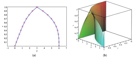
Figure 1. (a) Approximate solution of GLM (circle) and exact solution (line) at $t=1.0$; (b) 3D-plot of GLM for Problem 1.

Table 3. Comparison between GLM and existing methods for solving Problem 1.

	GLM		RK		VIM	HPM
r	$E^{-}(t=0.5;r)$	$E^{-}(t=1;r)$	$E^{-}(t=0.5;r)$	$E^{-}(t=1;r)$	$E^{-}(t=0.5;r)$	$E^{-}(t=0.5;r)$
0.0	0	0	0	0	0	0
0.1	9.956810(−11)	1.209550(−9)	4.823713(−10)	7.462263(−9)	7.6675(−11)	2.5125(−6)
0.2	1.992855(−10)	2.420914(−9)	9.654662(−10)	1.493572(−8)	1.5347(−10)	5.0288(−6)
0.3	2.998988(−10)	3.643163(−9)	1.452902(−9)	2.247632(−8)	2.3095(−10)	7.5676(−6)
0.4	4.033500(−10)	4.899886(−9)	1.954086(−9)	3.022960(−8)	3.1061(−10)	1.0178(−5)
0.5	5.133730(−10)	6.236430(−9)	2.487103(−9)	3.847537(−8)	3.9534(−10)	1.2954(−5)
0.6	6.360880(−10)	7.727180(−9)	3.081621(−9)	4.767250(−8)	4.8984(−10)	1.6051(−5)
0.7	7.806100(−10)	9.482820(−8)	3.781770(−9)	5.850381(−8)	6.0113(−10)	1.9698(−5)
0.8	9.596280(−10)	1.165754(−8)	4.649055(−9)	7.192064(−8)	7.3899(−10)	2.4215(−5)
0.9	1.190025(−9)	1.445635(−8)	5.765231(−9)	8.918787(−8)	9.1641(−10)	3.0029(−5)
1.0	1.493445(−9)	1.814234(−8)	7.235207(−9)	1.119283(−7)	1.1501(−9)	3.7686(−5)
r	$E^{+}(t=0.5;r)$	$E^{+}(t=1;r)$	$E^{+}(t=0.5;r)$	$E^{+}(t=1;r)$	$E^{+}(t=0.5;r)$	$E^{+}(t=0.5;r)$
0.0	2.986892(−9)	3.628465(−8)	1.447042(−8)	2.238567(−7)	2.3001(−9)	7.5371(−5)
0.1	2.985401(−9)	3.626651(−8)	1.446318(−8)	2.237446(−7)	2.2990(−9)	7.5333(−5)
0.2	2.974945(−9)	3.613950(−8)	1.441254(−8)	2.229612(−7)	2.2909(−9)	7.5070(−5)
0.3	2.946571(−9)	3.579484(−8)	1.427506(−8)	2.208346(−7)	2.2691(−9)	7.4354(−5)
0.4	2.891310(−9)	3.512354(−8)	1.400736(−8)	2.166932(−7)	2.2265(−9)	7.2959(−5)
0.5	2.800214(−9)	3.401690(−8)	1.356601(−8)	2.098656(−7)	2.1564(−9)	7.0660(−5)
0.6	2.664307(−9)	3.236592(−8)	1.290761(−8)	1.996801(−7)	2.0517(−9)	6.7231(−5)
0.7	2.474641(−9)	3.006184(−8)	1.198874(−8)	1.854652(−7)	1.9057(−9)	6.2444(−5)
0.8	2.222250(−9)	2.699583(−8)	1.076599(−8)	1.665493(−7)	1.7113(−9)	5.6076(−5)
0.9	1.898170(−9)	2.305891(−8)	9.195954(−8)	1.422609(−7)	1.4617(−9)	4.7899(−5)
1.0	1.493445(−9)	1.814234(−8)	7.235207(−8)	1.119283(−7)	1.1501(−9)	3.7686(−5)

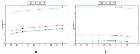
Figure 2. (a) Graph of Log (Error) versus r at $t=0.5$ for left bound of solutions; (b) Graph of Log (Error) versus r at $t=0.5$ for right bound of solutions for Problem 1.

8.2. Problem 2

Consider the following FVIDEs (see [12])

$$\begin{array}{cc}\hfill y^{\prime }\left(t\right)& =C+{\int }_0^{t}y(s;r)ds,\hfill \\ \hfill C& =[r-1,1-r],y\left(0\right)=[0,0],0\le s\le t\le 1.\hfill \end{array}$$

The equivalent system of ODEs based on (i)-differentiability:

$$\begin{array}{cc}\hfill {\left(y^{-}\right)}^{\prime }(t;r)& =(r-1)+{\int }_0^t{y}^{-}(s;r)ds,y^{-}(0;r)=0,\hfill \\ \hfill {\left(y^{+}\right)}^{\prime }(t;r)& =(1-r)+{\int }_0^t{y}^{+}(s;r)ds,y^{+}(0;r)=0.\hfill \end{array}$$

Exact solutions:

$$\begin{array}{cc}\hfill {\tilde{Y}}^{-}(t;r)& =(r-1)sinh\left(t\right),\hfill \\ \hfill {\tilde{Y}}^{+}(t;r)& =(1-r)sinh\left(t\right).\hfill \end{array}$$

For Problem 2, the graph of approximate solutions and 3D-plot of GLM are represented in Figure 3. Table 4 and Figure 4, show the numerical results using GLM compared with RK method.

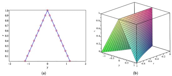
Figure 3. (a) Approximate solution of GLM (circle) and exact solution (line) at $t=1.0$; (b) 3D-plot of GLM for Problem 2.

Table 4. Comparison between GLM and RK for solving Problem 2.

	GLM		RK
r	$E^{-}(t=0.5;r)$	$E^{-}(t=1;r)$	$E^{-}(t=0.5;r)$	$E^{-}(t=1;r)$
0.0	2.069650(−10)	8.391900(−10)	1.431575(−9)	6.462170(−9)
0.1	1.862700(−10)	7.552900(−10)	1.288422(−9)	5.815940(−9)
0.2	1.655720(−10)	6.713560(−10)	1.145253(−9)	5.169731(−9)
0.3	1.655720(−10)	5.874450(−10)	1.145253(−9)	4.523523(−9)
0.4	1.241780(−10)	5.035170(−10)	8.589440(−10)	3.877302(−9)
0.5	1.034820(−10)	4.195950(−10)	7.157840(−10)	3.231079(−9)
0.6	8.278600(−11)	3.356810(−10)	5.726270(−10)	2.584868(−9)
0.7	6.208900(−11)	2.517620(−10)	4.294700(−10)	1.938651(−9)
0.8	4.139400(−11)	1.678420(−10)	2.863150(−10)	1.292426(−9)
0.9	2.069650(−11)	8.391900(−10)	1.431575(−10)	6.462170(−9)
1.0	0	0	0	0
r	$E^{+}(t=0.5;r)$	$E^{+}(t=1;r)$	$E^{+}(t=0.5;r)$	$E^{+}(t=1;r)$
0.0	2.069650(−10)	8.391900(−10)	1.431575(−9)	6.462170(−9)
0.1	1.862700(−10)	7.552900(−10)	1.288422(−9)	5.815940(−9)
0.2	1.655720(−10)	6.713560(−10)	1.145253(−9)	5.169731(−9)
0.3	1.448800(−10)	5.874450(−10)	1.002105(−9)	4.523523(−9)
0.4	1.241780(−10)	5.035170(−10)	8.589440(−10)	3.877302(−9)
0.5	1.034820(−10)	4.195950(−10)	7.157840(−10)	3.231079(−9)
0.6	8.278600(−11)	3.356810(−10)	5.726270(−10)	2.584868(−9)
0.7	6.208900(−11)	2.517620(−10)	4.294700(−10)	1.938651(−9)
0.8	4.139400(−11)	1.678420(−10)	2.863150(−10)	1.292426(−9)
0.9	2.069650(−11)	8.391900(−10)	1.431575(−10)	6.462170(−9)
1.0	0	0	0	0

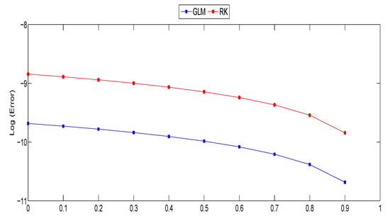
Figure 4. Graph of Log (Error) versus r at $t=0.5$ for left bound of solutions and right bound of solutions for Problem 2.

8.3. Problem 3

Consider the following FVIDEs (see [23])

$$\begin{array}{cc}\hfill y^{\prime }\left(t\right)& =C+{\int }_0^t(-y\left(s\right))ds,\hfill \\ \hfill C& =\left[2\right(r-2)sin(t),2(2-3r)sin(t\left)\right],y\left(0\right)=[3r-2,2-r],0\le t\le 1.\hfill \end{array}$$

The equivalent system of ODEs based on (i)-differentiability:

$$\begin{array}{cc}\hfill {\left(y^{-}\right)}^{\prime }(t;r)& =2(r-2)sin\left(t\right)+{\int }_0^1(-1)y^{+}(s;r)ds,y^{-}(0;r)=3r-2,\hfill \\ \hfill {\left(y^{+}\right)}^{\prime }(t;r)& =2(2-3r)sin\left(t\right)+{\int }_0^1(-1)y^{-}(s;r)ds,y^{+}(0;r)=2-r.\hfill \end{array}$$

Exact solutions based on (i)-differentiability:

$$\begin{array}{cc}\hfill {\tilde{Y}}^{-}(t;r)& =-rtsin\left(t\right)+(2-r)cos\left(t\right)+2(r-1)(exp(t)+exp(-t\left)\right),\hfill \\ \hfill {\tilde{Y}}^{+}(t;r)& =-rtsin\left(t\right)+(3r-2)cos\left(t\right)+2(1-r)(exp(t)+exp(-t\left)\right).\hfill \end{array}$$

The equivalent system of ODEs based on (ii)-differentiability:

$$\begin{array}{cc}\hfill {\left(y^{-}\right)}^{\prime }(t;r)& =2(2-3r)sin\left(t\right)+{\int }_0^1(-1)y^{-}(s;r)ds,y^{-}(0;r)=3r-2,\hfill \\ \hfill {\left(y^{+}\right)}^{\prime }(t;r)& =2(r-2)sin\left(t\right)+{\int }_0^1(-1)y^{+}(s;r)ds,y^{+}(0;r)=2-r.\hfill \end{array}$$

Exact solutions based on (ii)-differentiability:

$$\begin{array}{cc}\hfill {\tilde{Y}}^{-}(t;r)& =(3r-2)(cos(t)-tsin(t\left)\right),\hfill \\ \hfill {\tilde{Y}}^{+}(t;r)& =(2-r)(cos(t)-tsin(t\left)\right).\hfill \end{array}$$

For Problem 3, the graph of approximate solution compared with exact solution is given in Figure 5. Also the numerical results of GLM are compared with RK method using the both types of differentiabilities. The comparison of obtained results based on type (i)-differentiability are presented in Table 5 and Figure 6 whereas the results obtained based on type (ii)-differentiability are given in Table 6 and Figure 7. 3D-plots of GLM based on types (i) and (ii)-differentiability are shown in Figure 8.

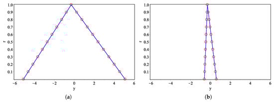
Figure 5. (a) Approximate solution of GLM (circle) and exact solution (line) at $t=1.0$ using type (i)-differentiability; (b) Approximate solution of GLM (circle) and exact solution (line) at $t=1.0$ using type (ii)-differentiability for Problem 3.

Table 5. Comparison between GLM and RK for solving Problem 3 based on (i)-differentiability.

	GLM		RK
r	$E^{-}(t=0.5;r)$	$E^{-}(t=1;r)$	$E^{-}(t=0.5;r)$	$E^{-}(t=1;r)$
0.0	9.591260(−9)	1.703350(−8)	3.884529(−8)	8.745231(−8)
0.1	8.252610(−9)	1.499912(−8)	3.333684(−8)	7.665465(−8)
0.2	6.913930(−9)	1.296471(−8)	2.782840(−8)	6.585705(−8)
0.3	5.575350(−9)	1.093031(−8)	2.231994(−8)	5.505935(−8)
0.4	4.236740(−9)	8.895910(−9)	1.681141(−8)	4.426157(−8)
0.5	2.898090(−9)	6.861520(−9)	1.130299(−8)	3.346385(−8)
0.6	1.559467(−9)	4.827130(−9)	5.794547(−9)	2.266616(−8)
0.7	2.208310(−10)	2.792740(−9)	2.860890(−10)	1.186848(−8)
0.8	1.117786(−9)	7.583400(−9)	5.222359(−9)	1.070790(−8)
0.9	2.456414(−9)	1.276027(−9)	1.073082(−8)	9.726932(−8)
1.0	3.795042(−9)	3.310421(−9)	1.623928(−8)	2.052464(−8)
r	$E^{+}(t=0.5;r)$	$E^{+}(t=1;r)$	$E^{+}(t=0.5;r)$	$E^{+}(t=1;r)$
0.0	9.591260(−9)	1.703350(−8)	3.884529(−8)	8.745231(−8)
0.1	9.011600(−9)	1.566117(−8)	3.658467(−8)	8.075957(−8)
0.2	8.431990(−9)	1.428888(−8)	3.432415(−8)	7.406693(−8)
0.3	7.852400(−9)	1.291656(−8)	3.206350(−8)	6.737409(−8)
0.4	7.272740(−9)	1.154423(−8)	2.980293(−8)	6.068132(−8)
0.5	6.693130(−9)	1.017195(−8)	2.754225(−8)	5.398850(−8)
0.6	6.113500(−9)	8.799650(−9)	2.528165(−8)	4.729569(−8)
0.7	5.533890(−9)	7.427330(−9)	2.302113(−8)	4.060305(−8)
0.8	4.954250(−9)	6.054989(−9)	2.076049(−8)	3.391018(−8)
0.9	4.374664(−9)	4.682732(−9)	1.849986(−8)	2.721740(−8)
1.0	3.795042(−9)	3.310421(−9)	1.623928(−8)	2.052464(−8)

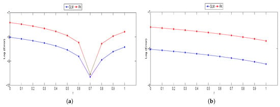
Figure 6. (a) Graph of Log (Error) versus r at $t=0.5$ for left bound of solutions using type (i)-differentiability; (b) Graph of Log (Error) versus r at $t=0.5$ for right bound of solutions using type (i)-differentiability for Problem 3.

Table 6. Comparison between GLM and RK for solving Problem 3 based on (ii)-differentiability.

	GLM		RK
r	$E^{-}(t=0.5;r)$	$E^{-}(t=1;r)$	$E^{-}(t=0.5;r)$	$E^{-}(t=1;r)$
0.0	7.590100(−9)	6.620856(−9)	3.247856(−8)	4.104928(−8)
0.1	6.451570(−9)	5.627722(−9)	2.760677(−8)	3.489188(−8)
0.2	5.313055(−9)	4.634590(−9)	2.273503(−8)	2.873452(−8)
0.3	4.174528(−9)	3.641453(−9)	1.786324(−8)	2.257713(−8)
0.4	3.036036(−9)	2.648343(−9)	1.299143(−8)	1.641972(−8)
0.5	1.897518(−9)	1.655208(−9)	8.119643(−9)	1.026232(−8)
0.6	7.590100(−10)	6.620856(−10)	3.247856(−9)	4.104928(−9)
0.7	3.795042(−10)	3.310421(−10)	1.623928(−9)	2.052464(−9)
0.8	1.518015(−9)	1.324166(−9)	6.495721(−9)	8.209863(−8)
0.9	2.656530(−9)	2.317297(−9)	1.136750(−8)	1.436725(−8)
1.0	3.795042(−9)	3.310421(−9)	1.623928(−8)	2.052464(−8)
r	$E^{+}(t=0.5;r)$	$E^{+}(t=1;r)$	$E^{+}(t=0.5;r)$	$E^{+}(t=1;r)$
0.0	7.590100(−9)	6.620856(−9)	3.247856(−8)	4.104928(−8)
0.1	7.210590(−9)	6.289804(−9)	3.085463(−8)	3.899682(−8)
0.2	6.831070(−9)	5.958752(−9)	2.923064(−8)	3.694430(−8)
0.3	6.451570(−9)	5.627722(−9)	2.760677(−8)	3.489188(−8)
0.4	6.072060(−9)	5.296667(−9)	2.598287(−8)	3.283943(−8)
0.5	5.692550(−9)	4.965625(−9)	2.435890(−8)	3.078694(−8)
0.6	5.313055(−9)	4.634590(−9)	2.273503(−8)	2.873452(−8)
0.7	4.933553(−9)	4.303548(−9)	2.111106(−8)	2.668203(−8)
0.8	4.554036(−9)	3.972496(−9)	1.948713(−8)	2.462956(−8)
0.9	4.174528(−9)	3.641453(−9)	1.786324(−8)	2.257713(−8)
1.0	3.795042(−9)	3.310421(−9)	1.623928(−8)	2.052464(−8)

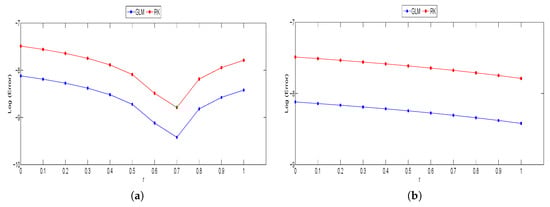
Figure 7. (a) Graph of Log (Error) versus r at $t=0.5$ for left bound of solutions using type (ii)-differentiability; (b) Graph of Log (Error) versus r at $t=0.5$ for right bound of solutions using type (ii)-differentiability for Problem 3.

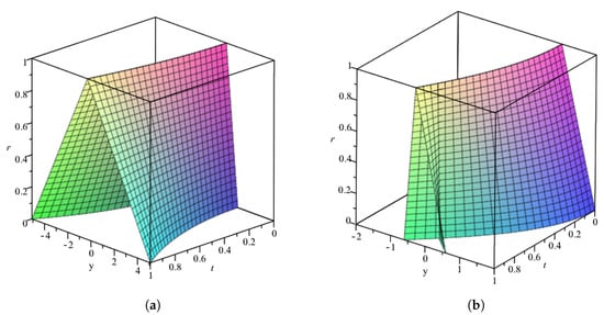
Figure 8. (a) 3D-plot of GLM using type (i)-differentiability for Problem 3; (b) 3D-plot of GLM using type (ii)-differentiability for Problem 3.

9. Discussion and Conclusions

Using the fuzzy GLM and fuzzy RK derived in this paper, the three FVIDEs given in Problems 1–3 are solved and the numerical results are shown. In addition, the obtained numerical results are compared with two other existing methods, variational iteration method and homotopy perturbation method, for Problem 1 at $t=0.5$.

For Problem 1, in Table 3, it is observed that the left bound of errors at $t=0.5$ obtained by the fuzzy GLM is competitive with the fuzzy RK for $r=0.2,0.9,1.0$. At $t=1$, the left bound errors from the fuzzy GLM is comparable with fuzzy RK when $r=0.1,0.7,0.8,0.9$. However, for the rest of errors fuzzy GLM achieved better accuracy compared to fuzzy RK. Moreover, the errors for the right bound of fuzzy GLM at both $t=0.5$ and $t=1$ are found to be one decimal place better than the fuzzy RK method. Meanwhile, the results acquired by GLM are almost the same with the results acquired by VIM. In comparison between GLM and HPM, GLM clearly outperformed the HPM.

For Problem 2, in Table 4, the fuzzy GLM is competitive with the fuzzy RK only when $r=0.4$ and $r=0.5$, though for the rest of r-levels the fuzzy GLM outperformed the fuzzy RK again by one decimal place better. For Problem 3, both types of differentiability are applied to solve this problem. In Table 5 by using type (i)-differentiability, there are some competitive results between the fuzzy GLM and fuzzy RK. However, in Table 6 by using type (ii)-differentiability, for almost all r-levels the fuzzy GLM gave more accurate results than the fuzzy RK.

Graphical illustrations of approximated solutions by fuzzy GLM in comparison with the exact solutions and 3D-plots of GLM for solving FVIDEs are presented in Figure 1, Figure 3, Figure 5 and Figure 8. The graphs shown that the GLM performed the accurate results. Moreover, in Figure 5b the approximate solutions of GLM based on type (ii)-differentiability showed smaller bound compared to the solutions based on type (i)-differentiability in Figure 5a. Considering that there exists a negative function in Problem 3, therefore the (ii)-differentiability approach is preferred. Graphs of comparison in terms of errors at $t=0.5$ between fuzzy GLM and other methods are showed as well. The fuzzy GLM is seen competitive with the VIM in Figure 2 meanwhile from Figure 4, Figure 6, and Figure 7, the fuzzy GLM is the more accurate method than HPM and RK3.

In conclusion, the fuzzy GLM combined with Simpson’s II method and Lagrange interpolation polynomials is an efficient numerical method for solving FVIDEs.

References

- Khastan, A.; Ivaz, K. Numerical solution of fuzzy differential equations by Nyström method. Chaos Solitons Fractals 2009, 41, 859–868. [Google Scholar] [CrossRef]
- Abu-Arqub, O.; El-Ajou, A.; Momani, S.; Shawagfeh, N. Analytical solutions of fuzzy initial value problems by HAM. Appl. Math. Inf. Sci. 2013, 7, 1903. [Google Scholar] [CrossRef]
- Puri, M.L.; Ralescu, D.A. Differentials of fuzzy functions. J. Math. Anal. Appl. 1983, 91, 552–558. [Google Scholar] [CrossRef]
- Buckley, J.J.; Feuring, T. Fuzzy differential equations. Fuzzy Sets Syst. 2000, 110, 43–54. [Google Scholar] [CrossRef]
- Bede, B.; Gal, S.G. Generalizations of the differentiability of fuzzy-number-valued functions with applications to fuzzy differential equations. Fuzzy Sets Syst. 2005, 151, 581–599. [Google Scholar] [CrossRef]
- Goetschel, R.; Voxman, W. Elementary fuzzy calculus. Fuzzy Sets Syst. 1986, 18, 31–43. [Google Scholar] [CrossRef]
- Kaleva, O. Fuzzy differential equations. Fuzzy Sets Syst. 1987, 24, 301–317. [Google Scholar] [CrossRef]
- Friedman, M.; Ma, M.; Kandel, A. Numerical solutions of fuzzy differential and integral equations. Fuzzy Sets Syst. 1999, 106, 35–48. [Google Scholar] [CrossRef]
- Park, J.Y.; Jeong, J.U. On existence and uniqueness of solutions of fuzzy integrodifferential equations. Indian J. Pure Appl. Math. 2003, 34, 1503–1512. [Google Scholar]
- Hajighasemi, S.; Allahviranloo, T.; Khezerloo, M.; Khorasany, M.; Salahshour, S. Existence and uniqueness of solutions of fuzzy Volterra integro-differential equations. In Proceedings of the International Conference on Information Processing and Management of Uncertainty in Knowledge-Based Systems, Cadiz, Spain, 11–15 June 2010; pp. 491–500. [Google Scholar]
- Zeinali, M.; Shahmorad, S.; Mirnia, K. Fuzzy integro-differential equations: Discrete solution and error estimation. Iranian J. Fuzzy Syst. 2013, 10, 107–122. [Google Scholar]
- Mikaeilvand, N.; Khakrangin, S.; Allahviranloo, T. Solving fuzzy Volterra integro-differential equation by fuzzy differential transform method. In Proceedings of the 7th Conference of the European Society for Fuzzy Logic and Technology, Aix-Les-Bains, France, 18–22 July 2011; Atlantis Press: Paris, France, 2011; pp. 891–896. [Google Scholar]
- Allahviranloo, T.; Abbasbandy, S.; Sedaghatfar, O. A New Method for Solving Fuzzy Integro-Differential Equation Under Generalized Differentiability. Neural Comput. Appl. 2012, 21, 191–196. [Google Scholar] [CrossRef]
- Allahviranloo, T.; Khezerloo, M.; Sedaghatfar, O.; Salahshour, S. Toward the existence and uniqueness of solutions of second-order fuzzy volterra integro-differential equations with fuzzy kernel. Neural Comput. Appl. 2013, 22, 133–141. [Google Scholar] [CrossRef]
- Matinfar, M.; Ghanbari, M.; Nuraei, R. Numerical solution of linear fuzzy Volterra integro-differential equations by variational iteration method. J. Intell. Fuzzy Syst. 2013, 24, 575–586. [Google Scholar]
- Sahu, P.K.; Saha Ray, S. Two-dimensional Legendre wavelet method for the numerical solutions of fuzzy integro-differential equations. J. Intell. Fuzzy Syst. 2015, 28, 1271–1279. [Google Scholar]
- Butcher, J.C. General linear methods. Acta Numer. 2006, 15, 157–256. [Google Scholar] [CrossRef]
- Rabiei, F.; Abd Hamid, F.; Rashidi, M.M.; Ismail, F. Numerical simulation of fuzzy differential equations using general linear method and B-series. Adv. Mech. Eng. 2017, 9, 1–16. [Google Scholar] [CrossRef]
- Bede, B. Mathematics of Fuzzy Sets and Fuzzy Logic; Springer: Berlin, Germany, 2013; 295p. [Google Scholar]
- Chalco-Cano, Y.; Román-Flores, H. On new solutions of fuzzy differential equations. Chaos Solitons Fractals 2008, 38, 112–119. [Google Scholar] [CrossRef]
- Linz, P. Analytical and Numerical Methods for Volterra Equations; Siam: Philadelphia, PA, USA, 1985; 227p. [Google Scholar]
- Butcher, J.C. Numerical Methods or Ordinary Differential Equations Second Edition; John Wiley and Sons: New York, NY, USA, 2008; 48p. [Google Scholar]
- Ghanbari, M. A new approach for solving fuzzy linear Volterra integro-differential equations. Iran. J. Fuzzy Syst. 2016, 13, 69–87. [Google Scholar]
© 2019 by the authors. Licensee MDPI, Basel, Switzerland. This article is an open access article distributed under the terms and conditions of the Creative Commons Attribution (CC BY) license (http://creativecommons.org/licenses/by/4.0/).