Dimensional Analysis under Pythagorean Fuzzy Approach for Supplier Selection

Abstract

The supplier appraisal process is one of the most important decision problems for companies focused on improving supply chain costs. Supplier selection is typically a multi-criteria decision making (MCDM) issue, as there is a lot of uncertain information. In order to overcome this issue, The Pythagorean Fuzzy Set is applied to handle the uncertainties involved in comparing the alternatives, criteria and opinions of decision makers. At the same time, a potential of Dimensional Analysis is a technique which deploys an association of the criteria capturing the interrelationship normally present in MCDM. In this sense, the purpose of this paper is to evaluate the suppliers in a supply chain cycle using Pythagorean Fuzzy Set and Dimensional Analysis. Finally, the applicability of the proposed method is illustrated through numerical examples, and a validation via Spearman correlation and Cronbach’s alpha.

1. Introduction

In today’s competitive world, the selection of suppliers has become a complicated problem that involves a large number of academics and professionals [1]. The selection of the provider depends on a variety of criteria such as characteristics of markets, demands from customers, delivery times, quality, price and service excellence [2,3]. Therefore, choosing the best suppliers can be conflicting in nature. According to Kang et al. [4], a supplier’s selection can be modeled as a typical multi-criteria decision making problem.

Moreover, various supplier selection methods such as Analytical Hierarchy Process (AHP), Analytic Network Process (ANP), Artificial Neural Network (ANN), Technique for Order Preference by Similarity to Idal Solution (TOPSIS), Data Envelopment Analysis (DEA), Integer programming, Genetic Algorithms and combinations of any of these tools are observed in the literature [1]. However, in decision making, most of these methods only consider quantitative criteria, and other type of factors—such as incomplete information, qualitative criteria and imprecision preferences—are not included [5].

In this context, the Fuzzy Set method has recently been applied for supplier selection [5]. As per a proposal from Jafarnejad and Aghasi [6], the integration of fuzzy Preference Ranking Organization Methods for Enrichment Evaluations (PROMETHEE) and linear programs for supplier selection under uncertainty. This is applicable in business to allow for the building of road maps for profit maximization. Mavi, Goh and Mavi [7] proposed a Shannon entropy and fuzzy TOPSIS, the first for weighing criteria and the second for ranking suppliers. Their findings show that demand risk is the most important factor. On other hand, Bolturk [8] developed the Pythagorean fuzzy extension of the COmbinative Distance-based Assessment (CODAS) method, which is applicable in supplier selection problems that are vague and imprecise. Additionally, the literature shows [5,6,9,10] that most of these methods such as AHP, TOPSIS—including fuzzy versions—and others have the following limitations:

• Do not take into account the interrelationship among three or more arguments.
• Limited qualitative criteria.
• Imprecise preferences of decision makers.

Dimensional Analysis (DA) is able to capture the interrelationship between multiple arguments (or criteria) into single dimensionless indexes [11], making it convenient in multi-criteria decision making (MCDM) problems with different measurement scales [11,12,13]. The main advantage of DA is that is can integrate the opinions of a group of decision makers (DM) on diverse information, such as alternatives, criteria and the importance of each criteria [11]. Nevertheless, DA is weak using quantitative (crisp) and qualitative (fuzzy) information, which is commonly present in MCDM problems.

On the other hand, Pythagorean Fuzzy Sets (PFS) have become a new generalization of fuzzy sets (FS) and can handle and model uncertain information in a more “flexible” way in the DM process than can Intuitionistic Fuzzy Sets (IFS). The main advantage of PFS is the condition that the square sum of their degree of membership and the degree of non-membership is equal to or less than $1$ [14,15,16,17,18,19,20,21]. For example, when a decision maker provides the evaluation information whose membership grade is 0.4 and the degree of non-membership is 0.9, an IFS cannot address this problem because 0.4 + 0.9 > 1. However, ${0.4}^2$ + ${0.9}^2$ < 1. That is, a PFS is able to represent this evaluation information [15].

Based on the aforementioned considerations, this research could have industrial application in medium and small enterprises, and may be directed to management, engineers and buyers that tackle the issue of supplier appraisal. Using an integrated tool: an extension of DA with PFS: the qualitative criteria, imprecision preferences of the DMs and interrelationship among the multi-input arguments can be overcame for multi-input arguments. The rest of the paper is organized as follows: In Section 2, the preliminaries of Pythagorean Fuzzy Sets (PFS) and Dimensional Analysis (DA) are given. In Section 3, the methodology of the integration of PFS and DA is given, and an algorithm is proposed in eight steps. In Section 4, two illustrated examples for supplier selection problems are presented, applying the proposed method. This approach is as follows: (1) A sensitivity analysis, (2) a comparative analysis with other fuzzy methods; in addition a Spearman correlation and Cronbach’s alpha in order to validate our method; (3) results. Finally, in Section 5, the conclusion is given and suggestions for further research are presented.

2. Preliminaries

2.1. Pythagorean Fuzzy Set (PFS)

Basic concepts of PFS are the following:

Definition 1.

[14,16,20], let X be a universe of discourse. Then IFS I in X is given by:

$$I=\{ \langle x, {\mu }_I(x), {\nu }_I (x)\rangle |x ϵ X\}.$$

(1)

Definition 2.

[17,20,21,22,23,24], let X be a universe of discourse. A PFS P in X is given by:

$$P=\{\langle x, {\mu }_P(x), {\nu }_P (x)\rangle |x ϵ X\}.$$

(2)

The degree of indeterminacy [14,16,23,24,25] is expressed, where ${\mu }_P :X \to \left[0,1\right]$ denotes the degree of membership and ${\nu }_P :X \to \left[0,1\right]$ denotes the degree of non-membership of the element $xϵX$ to the set $P$. Therefore, the degree of indeterminacy is given by:

$${\pi }_P (x)=\sqrt{1-{({\mu }_P (x))}^2-{({\nu }_P (x))}^2}.$$

(3)

According to Zhang and Xu [14], for convenience called $({\mu }_P (x), {\nu }_P (x))$ a PFS denoted by $p=({\mu }_P, {\nu }_P)$.

Definition 3.

[15,16,18];for any PFS,$p=(\mu , \nu )$,$p$is defined as follows:

$$s(p)={(\mu )}^2-{(\nu )}^2$$

(4)

where$s(p)ϵ\left[-1,1\right].$

Definition 4.

[14,16,18]; for any PFS,$p=(\mu , \nu )$, the accuracy is defined as follows:

$$a(p)={(\mu )}^2+{(\nu )}^2$$

(5)

where$a(p) ϵ \left[0,1\right].$

Definition 5.

[16,26], if M, N$\in$PFSs, and then the operations are defined as follows:

$$M^C =\{\langle x, {\nu }_M(x),{\mu }_M(x) \rangle |x \in X\}$$

(6)

$$M \subseteq N iff \forall x \in X,{\mu }_M(x) \le {\mu }_N(x) and {\nu }_M(x) \ge {\nu }_N(x)$$

(7)

$$M = N iff \forall x \in X,{\mu }_M(x) = {\mu }_N(x) and {\nu }_M(x) = {\nu }_N(x)$$

(8)

$${\Phi }_M =\{\langle x, 1, 0 \rangle |x \in X\}$$

(9)

$${\varnothing }_M =\{\langle x, 0, 1 \rangle |x \in X\}$$

(10)

$$M\cap N =\{\langle x,{\mu }_M(x)\wedge {\mu }_N(x),{\nu }_M(x)\vee {\nu }_N(x) \rangle |x \in X\}$$

(11)

$$M\cup N =\{\langle x,{\mu }_M(x)\vee {\mu }_N(x),{\nu }_M(x)\wedge V_N(x) \rangle |x \in X\}$$

(12)

$$M \oplus N \{\langle x, \sqrt{{\mu }_{M }^2(x)+ {\mu }_N^2(x)-{\mu }_M^2(x){\mu }_N^2(x)}, {\nu }_M(x){\nu }_N(x) \rangle |x \in X\};$$

(13)

$$\begin{array}{c}M\ominus N =\{\langle x, \sqrt{\frac{{\mu }_M^2 (x)- {\mu }_N^2 (x)}{1- {\mu }_N^2 (x)}}, \frac{{\nu }_M (x)}{{\nu }_N (x)} \rangle |x \in X\}, if {\mu }_M(x)\ge {\mu }_N(x),{\mu }_M(x)\\ \le min\{{\mu }_N(x), \frac{{\nu }_N (x){\pi }_M (x)}{{\pi }_N (x)} \}\end{array}$$

(14)

$$\begin{array}{c}M\oslash N =\{\langle x,\frac{{\mu }_M (x)}{{\mu }_N (x)} , \sqrt{\frac{{\nu }_M^2 (x)- {\nu }_N^2 (x)}{1- {\upsilon }_N^2 (x)}} \rangle |x \in X\}, if {\nu }_M(x)\ge {\nu }_N(x),{\mu }_M(x)\\ \le min\{{\mu }_N(x), \frac{{\mu }_N (x){\pi }_M (x)}{{\pi }_N (x)} \}\end{array}$$

(15)

$$p^{\lambda }=({\mu }^{\lambda }, \sqrt{1-(1-{\nu }^2{)}^{\lambda })}$$

(16)

$$M \otimes N =\{\langle x,{\mu }_M(x){\mu }_N(x), \sqrt{{\nu }_{M }^2(x)+ {\nu }_N^2- {\nu }_M^2 (x){\nu }_N^2(x)} \rangle |x \in X\}$$

(17)

$$\lambda p=(\sqrt{1-(1-{\mu }^2{)}^{\lambda }, {\nu }^{\lambda })}.$$

(18)

2.2. Dimensional Analysis (DA)

DA is a technique that has been used in the decision making process, particularly for the selection of multi-criteria-type alternatives. DA is an MCDM technique that assumes there is an optimal solution better than the rest, $S^{\ast }$. DA compares each alternative in evaluation with this ideal alternative to generate an index of similarity, therefore the highest index of similarity is chosen as the best alternative to the MCDM problem [11,12,13].

Definition 6.

Let$a_l^k(k=1,\dots ,n)(l=1,\dots m)$and$S_l^{\ast }= a_j^{\ast }(l=1,\dots ,m)$represent a database of crisp numbers. DA is defined as follows:

$$I{S}_i(a_1^i,a_2^i,\dots ,a_m^i)={\displaystyle \prod }_{j=1}^m{(\frac{a_j^i}{S_l^{\ast }})}^{w_j}$$

(19)

where$I{S}_i$is called the index of similarity for alternative i;$a_l^k$is the crisp evaluation of criterion l for alternative i;$S_l^{\ast }$is the crisp value of the ideal alternative for criterion l;$w_{j }(z=1,\dots ,m)$is the crisp weight for criterion l.

3. Methodology

In this section, we introduced the Pythagorean Fuzzy Dimensional Analysis (PFDA) approach for MCDM problems.

Based on Equation (18), the definition of PFDA is given as follows.

Definition 7.

Pythagorean Fuzzy Set Dimensional Analysis method. Let${\omega }_j^i=({\mu }_{w_j^i}, {\nu }_{w_j^i})(i=1,2,\dots n)(j=1,2\dots m)$and$S_j^i=({\mu }_{w_j^i}, {\nu }_{w_j^i})(j=1,2\dots m)$be a collection of P$F_s$, if

$$PFI{S}_i({\omega }_1^i, {\omega }_2^i,\dots , {\omega }_m^i)=({\otimes }_{j=1}^m (\frac{{\omega }_j^i}{S_j^{\ast }}{)}^{T_j})=({\otimes }_{j=1}^m{({\xi }_j^i)}^{T_j}),$$

(20)

then$PFI{S}_i$is named “Pythagorean Fuzzy Index of Similarity” for alternative$i$. Here,${\omega }_j^i$is the Pythagorean fuzzy evaluation of criterion$j$for alternative$i$,$S_j^{\ast }$is the Pythagorean fuzzy value of the “ideal alternative” for criterion$j$, and$T_j (j=1,2,\dots m)$is the corresponding crisp weight for criterion$j$satisfying$T_j>0 (j=1,2,\dots m)$and${\displaystyle \sum }_{j=1}^m{T}_j=1.$

Based on Equations (3)–(7) of the PFS described in Section 2, the next results can be derived.

Theorem 1.

Let${\xi }_j^i=({\mu }_{{\xi }_j^i},{\nu }_{{\xi }_j^i})(i=1,2,\dots ,n)(j=1,2,\dots ,m)$be a collection of PFS. Therefore, the aggregated value, by using$PFIS$is the following:

$$PFI{S}_i({\omega }_1^i,{\omega }_2^i,. . . .,{\omega }_m^i)=\left(\begin{array}{c}m\\ \otimes \\ j=1\end{array}{({\xi }_j^i)}^{T_j}\right)=\left({\displaystyle \prod }_{j=1}^m{\left({\mu }_{{\xi }_j^i}\right)}^{T_j},\sqrt{1-{\displaystyle \prod }_{j=1}^m{\left(1-{({\nu }_{{\xi }_j^i})}^2\right)}^{T_j}}\right).$$

(21)

Proof. 

Based on Equation (15) described in Section 2, we can obtained Equation (23):

$${\xi }_j^i=\frac{{\omega }_j^i}{S_j}=\left(\frac{{\mu }_{{\omega }_j^i}}{{\mu }_{{\omega }_j^{\ast }}},\frac{{\nu }_{{\omega }_j^i}-{\nu }_{{\omega }_j^{\ast }}}{1-{\nu }_{{\omega }_j^{\ast }}}\right)=\left({\mu }_{{\xi }_j^i},{\nu }_{{\xi }_j^i}\right).$$

(22)

Then, by Equation (16):

$${({\xi }_j^i)}^{T_j}=\left({\mu }_{{\xi }_j^i}{}^{T_j},\sqrt{1-{\left(1-{\nu }_{{\xi }_j^i}\right)}^{T_j}}\right).$$

(23)

Also, according to Equation (17):

$$\begin{array}{c}\begin{array}{c}m\\ \otimes \\ j=1\end{array}{({\xi }_j^i)}^{T_j}=\\ \left(({\mu }_{{\xi }_1^i}{}^{T_1})({\mu }_{{\xi }_2^i}{}^{T_j})\dots ({\mu }_{{\xi }_m^i}{}^{T_m}),\sqrt{1-({(1-{\nu }_{{\xi }_1^i}{}^2)}^{T_1}{(1-{\nu }_{{\xi }_2^i}{}^2)}^{T_j}\dots {(1-{\nu }_{{\xi }_m^i}{}^2)}^{T_j})}\right)=\\ \left({\displaystyle \prod }_{j=1}^m{({\mu }_{{\xi }_j^i})}^{T_j},\sqrt{1-{\displaystyle \prod }_{j=1}^m{(1-{({\nu }_{{\xi }_j^i})}^2)}^{T_j}}\right).\end{array}$$

(24)

This completes the proof of Theorem 1. □

When the MCDM problem contains both types of criteria, benefit criteria (BN) and cost criteria (C), the following has to be considered. If ${\alpha }_j\in BN$; then:

$${\xi }_j^i=\frac{{\alpha }_j^i}{S_j}=\left(\frac{{\mu }_{{\omega }_j^i}}{{\mu }_{{\omega }_j^{\ast }}},\sqrt{\frac{{\nu }_{{\omega }_j^i}-{\nu }_{\omega }}{1-{\nu }_{{\omega }_j^{\ast }}}}\right)=\left({\mu }_{{\xi }_j^i},{\nu }_{{\xi }_j^i}\right) j\in BN.$$

(25)

Otherwise, if ${\alpha }_j\in C$; then,

$${\xi }_j^{\prime i}=\frac{S_j}{{\alpha }_j^i}=\left(\frac{{\mu }_{{\omega }_j^{\ast }}}{{\mu }_{{\omega }_j^i}},\sqrt{\frac{{\nu }_{{\omega }_j^{\ast }}-{\nu }_{{\omega }_j^i}}{1-{\nu }_{{\omega }_j^i}}}\right)=\left({\mu }_{{\xi }_j^{\prime i}},{\nu }_{{\xi }_j^{\prime i}}\right) j\in C.$$

(26)

Following the next conditions,

$${\mu }_{{\omega }_j^{\ast }}=\left((\max {\mu }_{{\omega }_j^i} | j\in BN), (\min {\mu }_{{\omega }_j^i} | j\in C)\right)$$

(27)

$${\nu }_{{\omega }_j^{\ast }}=\left((\min {\nu }_{{\omega }_j^i} | j\in BN), (\max {\nu }_{{\omega }_j^i} | j\in C)\right),$$

(28)

where

$${\mathrm{S}}_{\mathrm{j}}=({\mathsf{\mu }}_{{\mathsf{\omega }}_{\mathrm{j}}^{\ast }},{\mathsf{\nu }}_{{\mathsf{\omega }}_{\mathrm{j}}^{\ast }}).$$

(29)

If $D{M}_k=\{{\mu }_k,{\nu }_k,{\pi }_k\}$ is a Pythagorean fuzzy number, the weight of DM [27] is represented by:

$${\epsilon }_k= \frac{({\mu }_k+ {\pi }_k({\mu }_k/({\mu }_k+{\nu }_k)))}{{\sum }_{k=1}^l({\mu }_k+{\pi }_k({\mu }_k/({\mu }_k+{\nu }_k)))}$$

(30)

where ${\sum }_{k=1}^l {\epsilon }_k=1$.

Preferences of the DM need to be gathered in a Pythagorean fuzzy matrix [27]:

$$\begin{array}{c}{X}_{kl}=PFWA(X_{kl}^{(1)}, X_{kl}^{(2)},\dots , X_{kl}^{(t)},\dots , X_{kl}^{(z)})= {\omega }_1{X}_{kl}^{(1)} \oplus {\omega }_2{X}_{kl}^{(2)}\oplus \dots \oplus {\omega }_z{X}_{kl}^{(z)}\oplus \dots \oplus \\ {\omega }_j{X}_{kl}^{(t)}=\left[ {\sum }_{k=1}^l ((\omega {\mu }_{kl}^{(z)}), (\omega {\nu }_{kl}^{(z)}))\right].\end{array}$$

(31)

The algorithm for proposed PF-DA below.

In accordance with above analysis, PF-DA is defined in the following steps:

• Step 1: Define the Pythagorean decision matrix.
• Step 2: Select the ideal solution in accordance with BN or C criteria values.
• Step 3: Establish criteria weights, use Equations (30) and (31).
• Step 4: Standardized matrix—use Equation (25) for BN criteria, Equation (26) for C criteria.
• Step 5: Standardized matrix elevated in accordance with criteria weights, use Equation (16).
• Step 6: Generate PFIS index, use Equation (21).
• Step 7: Establish the highest index of the index of similarity (IS), use Equation (4).
• Step 8: Establish the ranking, with highest values to lowest values.

4. Numerical Illustration

In this section, we consider a decision making problem that a manufacturing company is facing at Ciudad Juárez, Mexico. Mainly the problem is focused on supplier selection to achieve cost reductions at the finished goods manufacturing phase. The company is considering five suppliers for electronics items. Suppliers are defined by $A=\{A_1, A_2, A_3, A_4, A_5\}$. Four criteria involved are defined as:

• Price $(X_1)$: the most minimum values are selected.
• Facility $(X_2)$: great assessments are selected.
• Lead time $(X_3)$: high assessments are selected.
• Quality $(X_4)$: great assessments are selected.

Step 1: In accordance with DM evaluations, the Pythagorean fuzzy decision matrix is defined as follows:

$$\left[\begin{array}{cccc}\{0.10, 0.97\}& \{0.25, 0.90\}& \{1.00, 0.00\}& \{0.80, 0.44\}\\ \{0.40, 0.87\}& \{0.60, 0.71\}& \{0.50, 0.80\}& \{0.70, 0.60\}\\ \{0.96, 0.04\}& \{0.96, 0.04\}& \{0.96, 0.04\}& \{0.10, 0.97\}\\ \{0.71, 0.50\}& \{0.10, 0.97\}& \{0.10, 0.97\}& \{0.25, 0.92\}\\ \{0.50, 0.80\}& \{0.40, 0.87\}& \{0.71, 0.50\}& \{0.50, 0.80\}\end{array}\right].$$

(32)

Step 2: Establish the ideal solution in accordance with criteria values:

$$S^{+}:\{0.10, 0.97\} \{0.96, 0.04\} \{1.00, 0.00\} \{0.80, 0.44\}.$$

(33)

Step 3: Establish the criteria weights, use Equations (30) and (31):

$$W_{\{X_1, X_2, X_3, X_4\}}= \left[\begin{array}{c}\{0.24\}\\ \{0.24\}\\ \{0.22\}\\ \{0.31\}\end{array}\right].$$

(34)

Step 4: In order to standardize the matrix, use Equations (25) and (26) in accordance with BN or C:

$$\left[\begin{array}{cccc}\{1.0000, 0.0000\}& \{0.2604, 0.8998\}& \{1.0000, 0.0000\}& \{1.0000, 0.0000\}\\ \{0.2500, 0.6564\}& \{0.6250, 0.7094\}& \{0.5000, 0.8000\}& \{0.8750, 0.4543\}\\ \{0.1042, 0.9692\}& \{1.0000, 0.0000\}& \{0.9600, 0.0400\}& \{0.1250, 0.9627\}\\ \{0.1408, 0.8585\}& \{0.1042, 0.9700\}& \{1.0000, 0.9700\}& \{0.3125, 0.8997\}\\ \{0.2000, 0.7139\}& \{0.4167, 0.8698\}& \{0.7100, 0.5000\}& \{0.6250, 0.7440\}\end{array}\right]$$

(35)

Step 5: Then, each criteria column in the standardized matrix is elevated with criteria weights; use Equation (16):

$$\left[\begin{array}{cccc}\{1.0000, 0.0000\}& \{0.7240, 0.5731\}& \{1.0000, 0.0000\}& \{1.0000, 0.0000\}\\ \{0.7170, 0.3557\}& \{0.8930, 0.3932\}& \{0.8590, 0.4487\}& \{0.9590, 0.2629\}\\ \{0.5811, 0.6997\}& \{1.0000, 0.0000\}& \{0.9910, 0.0188\}& \{0.5250, 0.7451\}\\ \{0.6247, 0.5237\}& \{0.5810, 0.7019\}& \{0.6030, 0.6806\}& \{0.6970, 0.6340\}\\ \{0.6796, 0.3965\}& \{0.8100, 0.5362\}& \{0.9270, 0.2476\}& \{0.8640, 0.4703\}\end{array}\right]$$

(36)

Step 6: Then, to generate an index of similarity, $PFI{S}_i$, use Equation (21):

$$\left[\begin{array}{cc}0.7240& 0.5730\\ 0.5276& 0.6720\\ 0.3023& 0.8790\\ 0.1525& 0.9390\\ 0.4416& 0.7490\end{array}\right].$$

(37)

Step 7: To obtain the highest index of similarity, use Equation (4):

$$\left[\begin{array}{c}0.1958\\ -0.1726\\ -0.6817\\ -0.8585\\ -0.3661\end{array}\right].$$

(38)

Step 8: Establish the ranking; the results reveal that:

$$A_1> A_2> A_5> A_3> A_4.$$

Therefore $A_1$ is selected as the best supplier, and the highest index of similarity is chosen as the best alternative.

Illustration Example 2

In this example taken from the literature [8], an entrepreneur wants to select a supplier. Suppliers are defined by $P=\{P_1, P_2, P_3, P_4, P_5\}$, and the evaluation criteria are defined as:

• Product Quality $(X_1)$: BN criteria.
• Delivery Compliance $(X_2)$: BN criteria.
• Price $(X_3)$: high assessment C criteria.
• Production Capability $(X_4)$: C criteria.
• Technological Capability $(X_5)$: C criteria.

Step 1: A linguistic evaluation process is preferred since expert’s opinions, and then the Pythagorean fuzzy decision matrix is defined by DMs:

$$\left[\begin{array}{ccccc}\{0.22, 0.65\}& \{0.47, 0.56\}& \{0.29, 0.51\}& \{0.55, 0.76\}& \{0.28, 0.69\}\\ \{0.67, 0.20\}& \{0.23, 0.73\}& \{0.39, 0.45\}& \{0.61, 0.70\}& \{0.37, 0.61\}\\ \{0.41, 0.49\}& \{0.42, 0.59\}& \{0.34, 0.41\}& \{0.65, 0.68\}& \{0.48, 0.58\}\\ \{0.55, 0.48\}& \{0.63, 0.55\}& \{0.46, 0.40\}& \{0.67, 0.67\}& \{0.65, 0.57\}\end{array}\right].$$

(39)

Step 2: Establish the ideal solution in accordance with criteria values:

$$S^{+}:\{0.67, 0.20\} \{0.63, 0.55\} \{0.29, 0.51\} \{0.55, 0.76\}\{0.28, 0.69\}.$$

(40)

Step 3: Weights are assigned to each criterion by the experts:

$$W_{\{X_1, X_2, X_3, X_4\}}= \left[\begin{array}{c}\{0.25\}\\ \{0.10\}\\ \{0.50\}\\ \{0.10\}\\ \{0.05\}\end{array}\right].$$

(41)

Step 4: In order to standardize the matrix, use Equations (26) and (27) in accordance with BN or C:

$$\left[\begin{array}{ccccc}\{3.0455, 0.6312\}& \{1.3404, 0.1262\}& \{1.0000, 0.0000\}& \{1.0000, 0.0000\}& \{1.0000, 0.0000\}\\ \{1.0000, 0.2000\}& \{2.7391, 0.7300\}& \{1.3448, 0.2687\}& \{1.1091, 0.4144\}& \{1.3214, 0.4070\}\\ \{1.6341, 0.4900\}& \{1.5000, 0.5900\}& \{1.1724, 0.3326\}& \{1.1818, 0.4629\}& \{1.7143, 0.4588\}\\ \{1.2182, 0.4800\}& \{1.0000, 0.5500\}& \{1.5862, 0.0000\}& \{1.2182, 0.4833\}& \{2.3214, 0.4733\}\end{array}\right]$$

(42)

Step 5: Then, each criteria column in the standardized matrix is elevated with criteria weights; use Equation (18):

$$\left[\begin{array}{ccccc}\{1.3210, 0.3454\}& \{1.0297, 0.0400\}& \{1.0000, 0.0000\}& \{1.0000, 0.0000\}& \{1.0000, 0.0000\}\\ \{1.0000, 0.1008\}& \{1.1060, 0.2707\}& \{1.1597, 0.1918\}& \{1.0104, 0.1366\}& \{1.0140, 0.0949\}\\ \{1.1306, 0.2576\}& \{1.0414, 0.2047\}& \{1.0828, 0.2386\}& \{1.0168, 0.1544\}& \{1.0273, 0.1084\}\\ \{1.0506, 0.2517\}& \{1.0000, 0.1881\}& \{1.1294, 0.0000\}& \{1.0199, 0.1620\}& \{1.0430, 0.1122\}\end{array}\right]$$

(43)

Step 6: Then, to generate an index of similarity, $PFI{S}_i$, use Equation (22):

$$\left[\begin{array}{cc}1.3603& 0.3475\\ 1.3141& 0.3752\\ 1.3318& 0.4314\\ 1.4076& 0.3624\end{array}\right].$$

(44)

Step 7: To obtain the highest index of similarity, use Equation (4):

$$\left[\begin{array}{c}1.7297\\ 1.5862\\ 1.5875\\ 1.8499\end{array}\right].$$

(45)

Step 8: Establish the ranking; the results reveal that:

$$P_4> P_1> P_3> P_2.$$

Therefore $P_4$ is selected as the best supplier; the highest index of similarity is chosen as the best alternative.

4.1. Sensitivity Analysis

Different weights are assigned by changing the criteria weights to those obtained by PF-DA in order to observe how much it would influence the final rankings of alternatives. In the first example, we changed the weights of criteria as is shown in

Table 1. Example 1 sensitivity analysis.

C1	C2	C3	C4	Rankings
0.24	0.24	0.22	0.31	A1 > A2 > A5 > A3 > A4
0.25	0.25	0.25	0.25	A1 > A2 > A5 > A3 > A4
0.2	0.2	0.3	0.3	A1 > A2 > A5 > A3 > A4
0.3	0.3	0.2	0.2	A1 > A2 > A5 > A3 > A4
0.1	0.3	0.2	0.4	A1 > A2 > A5 > A3 > A4
0.5	0.2	0.15	0.15	A1 > A2 > A5 > A3 > A4

.

In the second example, we changed the weights of criteria as is shown in

Table 2. Example 2 sensitivity analysis.

C1	C2	C3	C4	C5	Rankings
0.25	0.1	0.5	0.1	0.05	P4 > P1 > P3 > P2
0.1	0.1	0.3	0.4	0.1	P4 > P2 > P3 > P1
0.15	0.15	0.3	0.2	0.2	P4 > P3 > P2 > P1
0.1	0.1	0.4	0.2	0.2	P4 > P2 > P3 > P1
0.3	0.1	0.15	0.15	0.3	P4 > P3 > P1 > P2
0.2	0.2	0.2	0.2	0.2	P3 > P4 > P2 > P1

.

4.2. Comparative Analysis

In accordance with example 1, using the PF-Multi-O bjective Optimization based on Ratio Analysis (MOORA) method, the results were the following:

$$A_1> A_2> A_3> A_5> A_4.$$

Furthermore, applying the PF-Technique for Order Preference by Similarity to Ideal Solution (TOPSIS) method [15], we obtained the following results in

Table 3. PF-TOPSIS closeness and rank.

$\mathit{D} ({\mathit{X}}_{\mathit{i}}, {\mathit{X}}^{-})$	$\mathit{D} ({\mathit{X}}_{\mathit{i}}, {\mathit{X}}^{+})$	$\mathbf{Closeness}({\mathit{X}}_{\mathit{i}})$	Rank
0.7063	0.2062	0.43059021	1
0.3355	0.3955	−1.23888967	2
0.4937	0.4743	−1.30058103	3
0.2427	0.8114	−3.4439003	5
0.3559	0.4981	−1.69490467	4

Then we have: $A_1>A_2>A_3>A_5>A_4$.

.

The Spearman correlation coefficient is based on the ranked values for each variable rather than the raw data. Spearman correlation is often used to evaluate relationships involving ordinal variables [28].

Table 4. Spearman correlation calculation for PF-DA, PF-MOORA and PF-TOPSIS.

Alternative	PF-DA Ranking	PF-MOORA Ranking	PF-TOPSIS Ranking	d	${\mathit{d}}^2$
A1	1	1	1	0	0
A2	2	2	2	0	0
A3	4	3	3	1	1
A4	5	5	5	0	0
A5	3	4	4	1	1

shows the rankings to calculate the Spearman correlation coefficient [28,29] is given by:

$$r_s=1-\frac{6\ast {{\displaystyle \sum }}_{i=1}^n{d}_i^2}{n^3-n}$$

(46)

When n = 5, and ${\displaystyle \sum }_{i=1}^n{d}_i^2=2$, then we have the following:

$${\mathrm{r}}_{\mathrm{s}}=1-\frac{6\ast 2}{5^3-5}=0.9.$$

(47)

On other hand, Cronbach’s alpha [30,31,32] is calculated using SPSS as is shown in

Table 5. Reliability statistics for PF-DA, PF-MOORA and PF-TOPSIS.

Cronbach’s Alpha	Cronbach’s Alpha Based on the Typified Elements	N of Elements
0.977	0.977	3

.

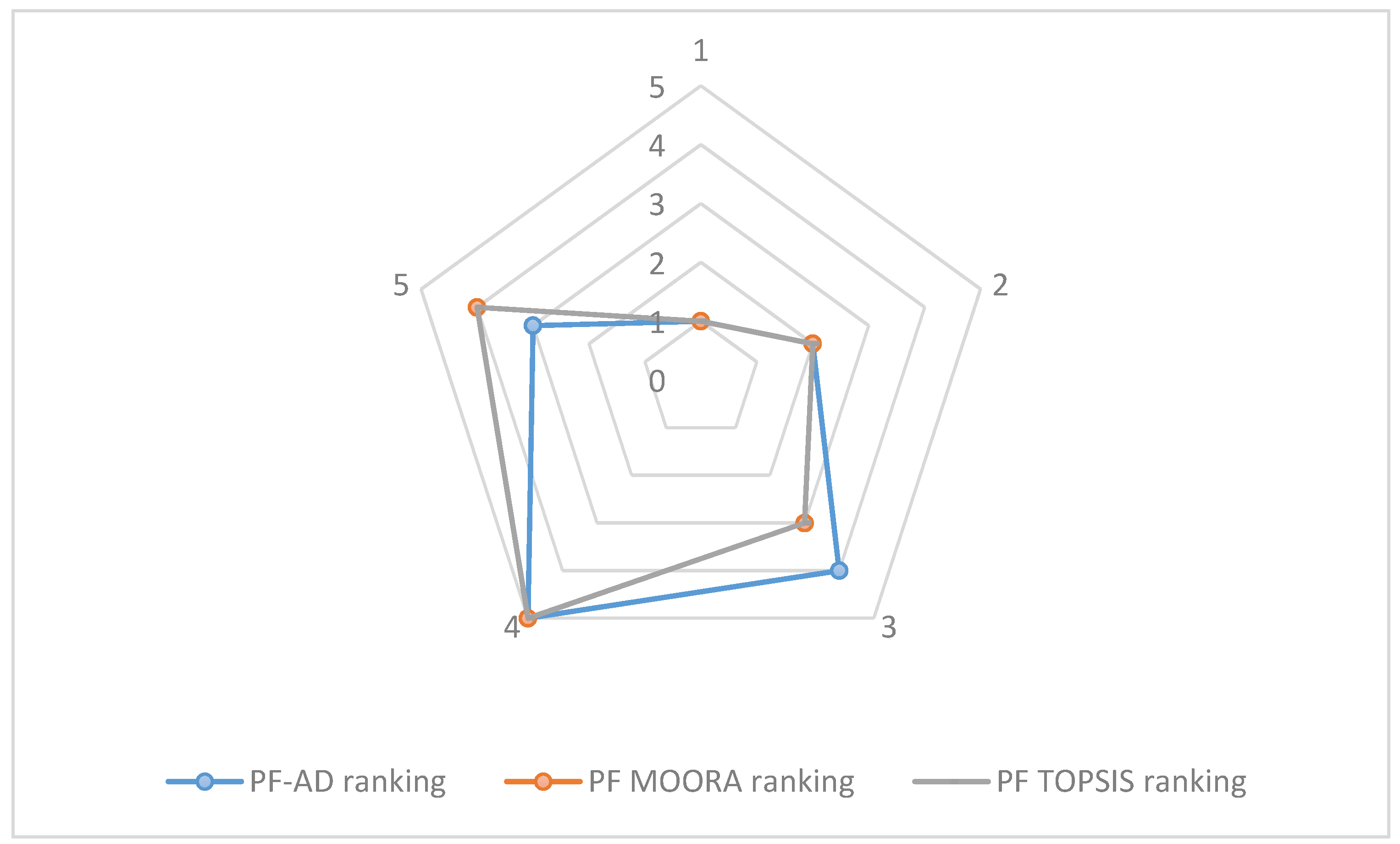
The Figure 1 is a graphic with the ranking comparison for PF-DA, PF MOORA and PF-TOPSIS.

In accordance with example 2, using the PF-CODAS method, the results show the following:

$$P_4> P_1> P_2> P_3.$$

Table 6. Spearman correlation calculation for PF-DA and PF-CODAS

Alternative	PF-DA Ranking	PF CODAS Ranking	d	${\mathit{d}}^2$
P1	4	4	0	0
P2	1	1	0	0
P3	3	2	1	1
P4	2	3	1	1

shows the rankings to calculate the Spearman correlation coefficient [28,29], for illustration example 2:

When n = 4, and ${\displaystyle \sum }_{i=1}^n{d}_i^2=2$, then we have the following:

$$r_s=1- \frac{6\ast 2}{4^3-4}=0.8.$$

(48)

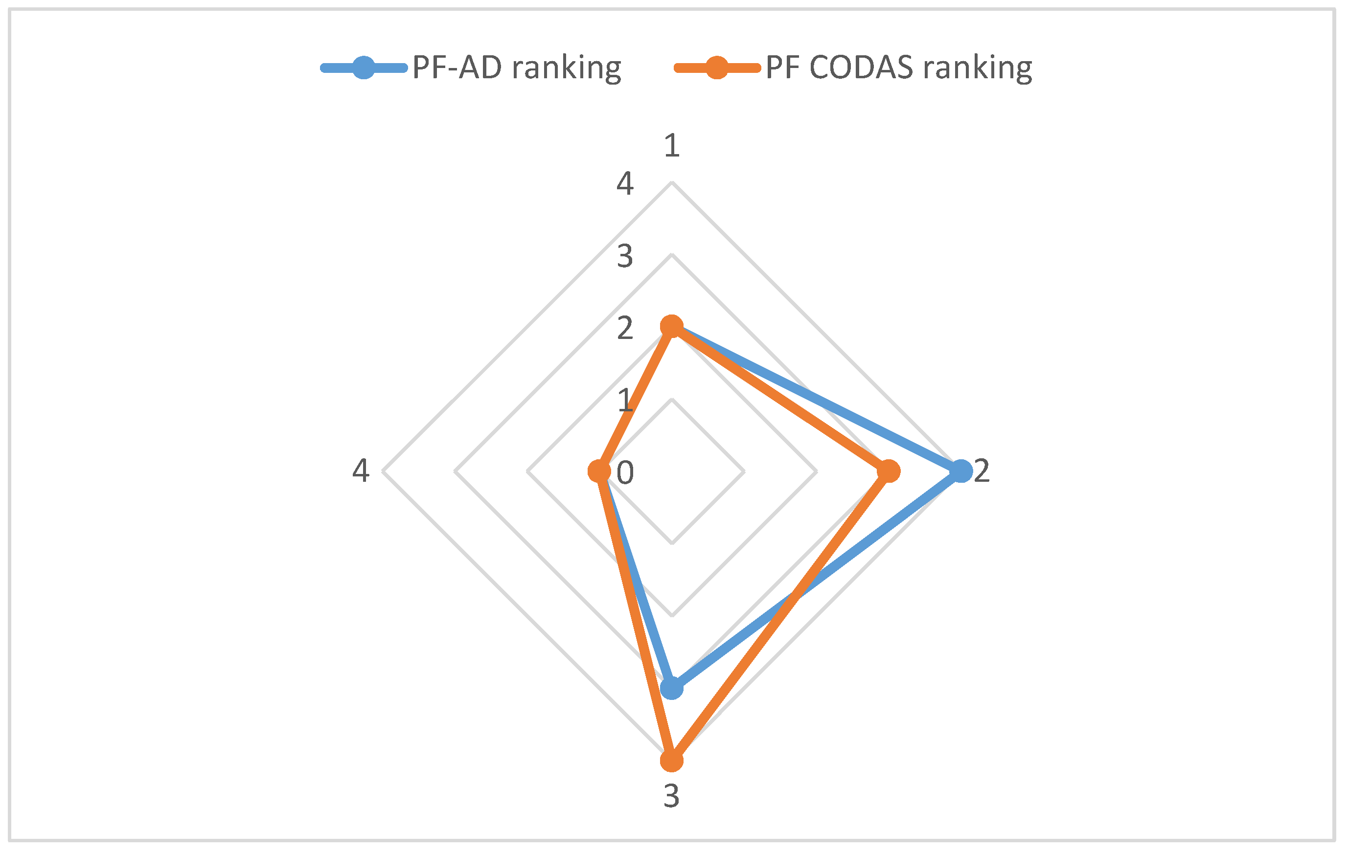
The Figure 2 is a graphic with the ranking comparison for PF-DA and PF-CODAS.

On other hand, Cronbach’s alpha [30,31,32] is calculated using SPSS as is shown in

Table 7. Reliability statistics for PF-DA and PF-CODAS.

Cronbach’s Alpha	N of Elements
0.889	2

.

4.3. Results

Due the PFS satisfies the condition that the square sum of their degree of membership and the degree of non-membership was equal to or less than 1 [14,16,17,18,19,20,21], the PFS is able to represent the evaluation information [15]; then we presented two illustrated examples using PFS.

In illustration example 1, for PF-DA, PF-MOORA and PF-TOPSIS, where $A_1$ was selected as the best supplier, the highest index of similarity was chosen as the optimal alternative. The result shows that the Spearman correlation was 0.9, which proved that there is a substantial correspondence between our approach, PF-DA, and the two MCDM approaches stated in the literature, namely PF-MOORA and PF-TOPSIS. On other hand, the Cronbach’s alpha was 0.977, which is a high value and indicates strong consistency [33]. This means that PF-DA is suitable for dealing with MCDM problems. Moreover, the integration of PF-DA provides advantages over PF-MOORA and PF-TOPSIS as DA attempts to integrate the opinions of a group of decision makers (DM) on diverse information, including alternatives, criteria and the importance of such criteria [11], whereas MOORA and TOPSIS do not.

On other hand, in illustration example 2, for PF-DA and PF-CODAS, $P_4$ was selected as the best supplier as it presented the highest index of similarity, indicating the optimal alternative. However, in CODAS the negative ideal solution is considered [8], while in DA the positive ideal solution is considered [11,12]. The Spearman correlation was 0.8, which means that there is substantial similarity between the PF-DA and PF-CODAS approaches. The Cronbach’s alpha was 0.889, which is a high value and indicates strong consistency [33].

5. Conclusions

In this paper we introduced a method of the Pythagorean Fuzzy Dimensional Analysis (PF-DA) in fuzzy forecasting decision problems. Forecasts are interesting because they can counteract adverse actions and simulate decisions. Therefore, it is necessary to use aggregation operators and methods that cope well with uncertainty and inaccuracy in forecasts [33]. In this sense, the DA method is extended with PFS in order to deal with commonly involved problems in MCDM such as the imprecise preferences of DMs and their interrelationships. Thus, the PF-DA method is developed in eight steps. Furthermore, the application of the proposed method is illustrated by numerical examples that demonstrate that the method is suitable for supplier selection. The Spearman correlation and Cronbach’s alpha values show that PF-DA is suitable to deal with MCDM problems. In future, works concerning PF-DA could focus on dealing with other kinds of MCDM problems such as: project selection, investment selection, machine selection, manufacturing systems, staff selection, etc.