Article

Analytic Loss Minimization: Theoretical Framework of a Second Order Optimization Method

by
Ioannis K. Dassios
AMPSAS, University College Dublin, Dublin 4, Ireland
Symmetry 2019, 11(2), 136; https://doi.org/10.3390/sym11020136
Submission received: 6 December 2018 / Revised: 14 January 2019 / Accepted: 22 January 2019 / Published: 26 January 2019

Abstract

:
In power engineering, the Y b u s is a symmetric N × N square matrix describing a power system network with N buses. By partitioning, manipulating and using its symmetry properties, it is possible to derive the K G L and Y G G M matrices, which are useful to define a loss minimisation dispatch for generators. This article focuses on the case of constant-current loads and studies the theoretical framework of a second order optimization method for analytic loss minimization by taking into account the symmetry properties of Y b u s . We define an appropriate matrix functional of several variables with complex elements and aim to obtain the minimum values of generator voltages.

1. Introduction

Electrical power system calculations rely heavily on Y b u s , a symmetric square N × N matrix, which describes a power system network with N buses. It represents the nodal admittance of the buses in a power system, see Figure 1.
By taking advantage of its symmetry properties, it is useful to split the Y b u s into sub-matrices and separately quantify the connectivity between load and generation nodes in the network; see [3]. This idea has been also further applied to several power engineering problems [4,5,6,7]. Currents ( I ) and voltages ( V ) in an electrical power system are related by the symmetric admittance matrix, Y b u s , in such a way as to group generator ( G ) and load ( L ) nodes separately (see [8,9]):
I G I L = Y b u s V G V L ,
where I G , V G C m , I L , V L C n and:
Y b u s = Y G G Y G L Y L G Y L L .
Since Y b u s is symmetric, we have Y L G = Y G L T ; where Y G G C m × m , Y L L C n × n , Y L G = Y G L T C n × m and n + m = N with n m . The kernel of Y b u s is known and has dimension one, unless the grid graph is disconnected. From this, one can conclude that Y L L is invertible. The use of a pseudo-inverse could be considered only if all nodes are loads. Let Z L L = Y L L 1 . Then, we can define ([10,11]) two useful sub-matrices:
Y G G M = Y G G + Y G L F L G ,
and:
F L G = Z L L Y L G = K G L T .
Using (2) and (3), we give (1) the form:
V L I G = Z L L F L G K G L Y G G M I L V G ,
from where more insightfully, one can use to derive an expression for this optimal generator dispatch:
I G = K G L I L + Y G G M V G .
Furthermore, by using these expressions, we can arrive at V G T I G = V G T K G L I L + V G T Y G G M V G and I L T V L = I L T Z L L I L + I L T F L G V G . Then (see [12,13,14]), given that generator powers will be positive and loads negative, the total system loss is given by the sum V G T I G + I L T V L = V G T Y G G M V G + V G T ( Y G L Z L L Y L G T Z L L T ) I L + I L T Z L L T I L . From the three components in this sum, the circulating current loss is directly a consequence of generator voltage mismatches, i.e., it depends on the product Y G G M V G . How may in general generator voltage mismatches be avoided? It is trivial to achieve a consistent Y G G M V G 1 profile, as voltage magnitudes are directly controlled by arbitrary set points using automatic reactive power control. Under minimum loss condition, the work in [4] implies that V G is homogeneous, and by obtaining the min Y G G M V G 1 , the second term of (4), corresponding to current circulated between generators, reduces with the ideal conditions being: I G = K G L I L S G O p t . This is equivalent to the loss-minimizing formula presented in [4] and gives two terms for I G , which the system operator can control by generator dispatch. We used · 1 because of its properties in robustness and sparsity. However, in general, the proposed method could also work by replacing this norm with · 2 . Loss minimization in power systems is usually achieved using optimization techniques. There are several methods in the literature that avoid matrix factorizations and have low memory requirements; however, in most of these methods, which are usually first order methods, essential information is missing, and practical convergence is slow. In this article, we propose a second order method that aims to be memory efficient, provide effective computational results and have noticeable progress towards a solution. Note that when loads are constant-power, their current I L becomes a function of their voltages, and therefore, the different terms in (4) cannot be treated independently. Hence, in a case like that, it would not be clear whether the proposed solution would minimize losses when constant-power loads are present. For this reason, in this article, we focus on and apply the results to the case of constant-current loads.

2. Mathematical Background

We are interested in the following optimization problem:
minimize Y G G M V G 1 , subject   to : A V G = b ,
where:
A = Y G G Y L G , b = I G I L Y G L Y L L V L ,
and Y G G M , Y G G C m × m , V G , I G Y G L V L C m , Y L L C n × n , V L , I L Y L L V L C n . Let:
Y G G M = W , and Y G G M V G = Y C m , with Y = y 1 y 2 y m .
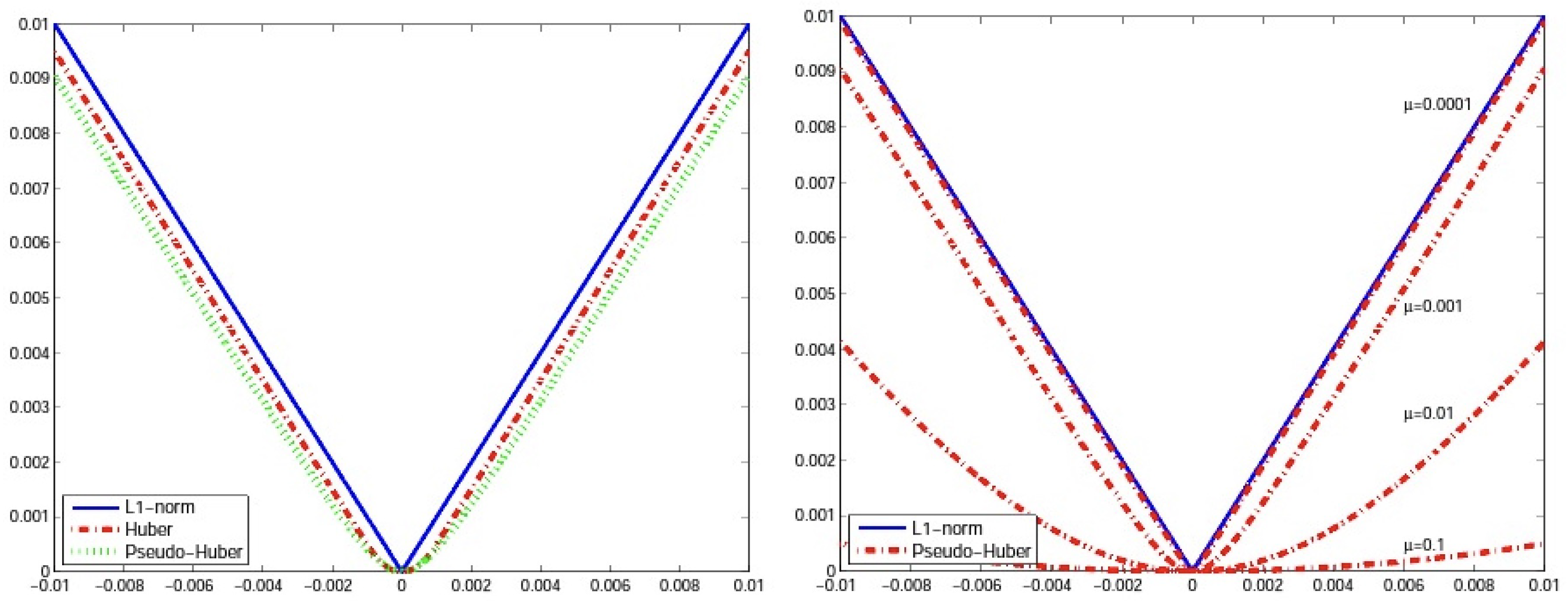
In the next section with the main results, we will apply a second order optimization method, i.e., we will use derivatives of first and second order. However, the 1 -norm is not differentiable. Many researchers in the literature use first order optimization methods and apply appropriate smoothing to the problem by using the Huber function. In our case, this is not possible since the Huber function is differentiable, but not twice differentiable. Hence, we propose to replace the 1 -norm with the pseudo-Huber function [15,16], see Figure 2. The pseudo-Huber function parametrized with μ > 0 is:
Ψ μ ( W V G ) = μ i = 1 m ( 1 + y i y ¯ i μ 2 1 ) .
The gradient of the pseudo-Huber function Ψ μ ( W V G ) is then given by:
Ψ μ ( W V G ) = 1 2 μ y 1 1 + y 1 y ¯ 1 μ 2 , , y m 1 + y m y ¯ m μ 2 , y ¯ 1 1 + y 1 y ¯ 1 μ 2 , , y ¯ m 1 + y m y ¯ m μ 2 W ¯ W
and the Hessian is given by:
2 Ψ μ ( W V G ) = 1 4 μ W ¯ T W T ( diag Y ^ 1 , , Y ^ m , Y ¯ ^ 1 , , Y ¯ ^ m W W ¯ +
+ diag Y 1 * , , Y m * , Y ¯ 1 * , , Y ¯ m * W ¯ W ) ,
where:
Y ^ i = 1 ( 1 + y 1 y ¯ 1 μ 2 ) 3 + 1 1 + y 1 y ¯ 1 μ 2
and:
Y i * = 1 μ 2 y i 2 ( 1 + y 1 y ¯ 1 μ 2 ) 3 .
The following lemma shows that the gradient of the function Ψ μ ( W V G ) is bounded.
Lemma 1.
The gradient Ψ μ ( W V G ) satisfies:
2 K m 1 m Ψ μ ( W V G ) 2 K m 1 m ,
where 1 m is a vector of ones of length m, and:
K = m a x 1 i m , 1 j n [ R e w i j , I m w i j ] .
Proof. 
Since:
( Re y i ) 2 ( μ ) 2 + ( Re y i ) 2 + ( Im y i ) 2 , and ( Im y i ) 2 ( μ ) 2 + ( Re y i ) 2 + ( Im y i ) 2
we get
1 μ y i 1 + y 1 y ¯ 1 μ 2 = Re y i μ 2 + y 1 y ¯ 1 + i Im y i μ 2 + y 1 y ¯ 1 ,
or equivalently,
1 μ y i 1 + y 1 y ¯ 1 μ 2 1 + i , and 1 μ y ¯ i 1 + y 1 y ¯ 1 μ 2 1 i .
Then,
Ψ μ ( W V G ) 1 2 [ 1 + i , , 1 + i , 1 i , , 1 i ] W ¯ W ,
or equivalently,
Ψ μ ( W V G )
1 2 [ ( 1 + i ) i = 1 m w ¯ i 1 + ( 1 i ) i = 1 m w i 1 , , ( 1 + i ) i = 1 m w ¯ i n + ( 1 i ) i = 1 m w i n ] ,
or equivalently,
Ψ μ ( W V G ) [ i = 1 m ( w ¯ i 1 + w i 1 ) , , i = 1 m ( w ¯ i n + w i n ) ] 2 K m 1 n .
Furthermore, in a similar way, it can be proven that 2 K m 1 n Ψ μ ( W V G ) . The proof is completed. □
Lemma 2.
The Hessian matrix 2 Ψ μ ( W V G ) satisfies:
0 I n 2 Ψ μ ( W V G ) 1 μ L I n ,
where L = 1 4 W ¯ T W T ( 2 W W ¯ + W ¯ W ) .
Proof. 
It is known that for every induced norm · , we have:
λ 2 Ψ μ ( W V G ) ,
where λ 0 is a random eigenvalue of 2 Ψ μ ( W V G ) . Observe that:
Y ^ i 1 ( 1 + y 1 y ¯ 1 μ 2 ) 3 + 1 1 + y 1 y ¯ 1 μ 2 2 ,
and:
Y i * = y i 2 μ 2 1 + y 1 y ¯ 1 μ 2 3 2 1
because:
y i 2 μ 2 1 + y 1 y ¯ 1 μ 2 ( 1 + y 1 y ¯ 1 μ 2 ) 3 2 .
Thus:
2 Ψ μ ( W V G )
1 4 μ W ¯ T W T ( diag Y ^ 1 , , Y ^ m , Y ¯ ^ 1 , , Y ¯ ^ m W W ¯ +
+ diag Y 1 * , , Y m * , Y ¯ 1 * , , Y ¯ m * W ¯ W ) ,
or equivalently,
2 Ψ μ ( W V G ) 1 μ L .
The proof is completed. □
The next lemma shows that the Hessian matrix of the pseudo-Huber function is Lipschitz continuous.
Lemma 3.
The Hessian matrix 2 Ψ μ ( W V G ) is Lipschitz continuous:
2 Ψ μ ( z ) 2 Ψ μ ( y ) 1 μ 2 M z y .
where:
M = 1 2 W ¯ T W T W W ¯ + 2 W ¯ T W T W ¯ W .
Proof. 
2 Ψ μ ( z ) 2 Ψ μ ( y ) = 0 1 2 Ψ μ ( y + s ( z y ) ) d s d s 0 1 2 Ψ μ ( y + s ( z y ) ) d s d s ,
or equivalently,
2 Ψ μ ( z ) 2 Ψ μ ( y ) 1 4 μ W ¯ T W T W W ¯ 0 1 d d s diag Z ^ 1 , , Z ^ m , Z ¯ ^ 1 , , Z ¯ ^ m d s + + 1 4 μ W ¯ T W T W ¯ W 0 1 d d s diag Z 1 * , , Z m * , Z ¯ 1 * , , Z ¯ m * d s . ,
where:
Z ^ i = 1 ( 1 + [ y i + s ( z i y i ) ] [ y ¯ i + s ( z ¯ i y ¯ i ) ] μ 2 ) 3 + 1 1 + [ y i + s ( z i y i ) ] [ y ¯ i + s ( z ¯ i y ¯ i ) ] μ 2 ,
and:
Z i * = 1 μ 2 [ y i + s ( z i y i ) ] 2 ( 1 + [ y i + s ( z i y i ) ] [ y ¯ i + s ( z ¯ i y ¯ i ) ] μ 2 ) 3 .
Furthermore:
d d s ( diag Z ^ 1 , , Z ^ m , Z ¯ ^ 1 , , Z ¯ ^ m ) =
= vec ( d d s ( diag Z ^ 1 , , Z ^ m , Z ¯ ^ 1 , , Z ¯ ^ m ) =
= max [ d d s ( diag Z ^ 1 , , Z ^ m , Z ¯ ^ 1 , , Z ¯ ^ m ) ] i i =
= max [ d d s 1 ( 1 + [ y i + s ( z i y i ) ] [ y ¯ i + s ( z ¯ i y ¯ i ) ] μ 2 ) 3 + 1 1 + [ y i + s ( z i y i ) ] [ y ¯ i + s ( z ¯ i y ¯ i ) ] μ 2 ] i i =
= max ( 3 2 1 ( 1 + [ y i + s ( z i y i ) ] [ y ¯ i + s ( z ¯ i y ¯ i ) ] μ 2 ) 5 1 2 ( 1 1 + [ y i + s ( z i y i ) ] [ y ¯ i + s ( z ¯ i y ¯ i ) ] μ 2 ) 3 ) ·
· ( 1 μ 2 ( [ y i + s ( z i y i ) ] [ y ¯ i z ¯ i ] + [ y i z i ] [ y ¯ i + s ( z ¯ i y ¯ i ) ] )
1 μ 2 z y max ( 3 2 [ y i + s ( z i y i ) ] ( 1 + [ y i + s ( z i y i ) ] [ y ¯ i + s ( z ¯ i y ¯ i ) ] μ 2 ) 5 + 1 2 [ y i + s ( z i y i ) ] 1 + [ y i + s ( z i y i ) ] [ y ¯ i + s ( z ¯ i y ¯ i ) ] μ 2 ) 3 +
+ [ 3 2 [ y ¯ i + s ( z ¯ i y ¯ i ) ] ( 1 + [ y i + s ( z i y i ) ] [ y ¯ i + s ( z ¯ i y ¯ i ) ] μ 2 ) 5 + 1 2 ( [ y ¯ i + s ( z ¯ i y ¯ i ) ] 1 + [ y i + s ( z i y i ) ] [ y ¯ i + s ( z ¯ i y ¯ i ) ] μ 2 ) 3 ) )
1 μ 2 z y μ 2 92 25 5 < 1 μ z y ,
or equivalently,
d d s ( diag Z ^ 1 , , Z ^ m , Z ¯ ^ 1 , , Z ¯ ^ m ) 1 μ z y
and:
d d s ( diag Z 1 * , , Z m * , Z ¯ 1 * , , Z ¯ m * ) =
= vec ( d d s ( diag Z 1 * , , Z m * , Z ¯ 1 * , , Z ¯ m * ) =
= max [ d d s ( diag Z 1 * , , Z m * , Z ¯ 1 * , , Z ¯ m * ) ] i i =
= max d d s ( 1 μ 2 [ y i + s ( z i y i ) ] 2 ( 1 + [ y i + s ( z i y i ) ] [ y ¯ i + s ( z ¯ i y ¯ i ) ] μ 2 ) 3 )
1 μ 2 y z max 2 [ y i + s ( z i y i ) ] ( 1 + [ y i + s ( z i y i ) ] [ y ¯ i + s ( z ¯ i y ¯ i ) ] μ 2 3 2 +
+ 3 μ 2 [ y i + s ( z i y i ) ] 3 ( 1 + [ y i + s ( z i y i ) ] [ y ¯ i + s ( z ¯ i y ¯ i ) ] μ 2 5 2
32 25 μ z y < 2 μ z y ,
or equivalently,
d d s ( diag Z 1 * , , Z m * , Z ¯ 1 * , , Z ¯ m * ) 2 μ z y .
From (8) and (9), we get:
2 Ψ μ ( z ) 2 Ψ μ ( y ) 1 4 μ W ¯ T W T W W ¯ 1 μ z y +
1 4 μ W ¯ T W T W ¯ W 2 μ z y ,
or equivalently,
2 Ψ μ ( z ) 2 Ψ μ ( y ) 1 μ 2 M z y ,
where:
M = 1 2 W ¯ T W T W W ¯ + 2 W ¯ T W T W ¯ W .
The proof is completed. □

3. Main Results

In this section, we will present our main results and the proposed optimization method. We begin with a proposition that will be useful in the main Theorem.
Proposition 1.
The ith row of the matrix Y G G M , given in (2), sums to d i , = 1 , 2 , , m ; where d i is the sum of the i th row of the matrix Y G G + Y G L as defined in (1).
Proof. 
From (3):
F L G = Z L L Y L G ,
whereby multiplying by 1 n , we get:
F L G 1 1 1 = Z L L Y L G 1 1 1 .
Let c i be the sum of the i th row of the matrix Y L L + Y L G as defined in (1). Then:
F L G 1 1 1 = Z L L ( c 1 c 2 c m Y L L 1 1 1 ) ,
or equivalently,
F L G 1 1 1 = Y L L 1 1 1 Z L L c 1 c 2 c m .
For the sum of each row of Y G G M , we have:
Y G G M 1 1 1 = ( Y G G + Y G L F L G ) 1 1 1 = Y G G 1 1 1 + Y G L ( 1 1 1 Z L L c 1 c 2 c m ) ,
or equivalently,
Y G G M 1 1 1 = ( Y G G + Y G L ) 1 1 1 Y G L Z L L c 1 c 2 c m ,
or equivalently, from [10]:
Y G G M 1 1 1 = d 1 d 2 d m .
The proof is completed. □
Theorem 1.
We consider the following optimization problem:
m i n i m i z e V G Y G G M V G 1 , s u b j e c t   t o : A V G = b ,
where:
A = Y G G Y L G , b = I G I L Y G L Y L L V L ,
and Y G G M , Y G G C m × m , I G Y G L V L C m , Y L G C n × m , I L Y L L V L C n . Then, by using a second order optimization method, an approximate solution of (10) in respect of V G C m is given by the solution of the linear system:
A ˜ V G = γ ψ μ ( Y G G M V G ( 0 ) ) + A * ( A V G ( 0 ) b ) + A ˜ V G ( 0 ) ,
where A ˜ = [ γ 2 ψ μ ( Y G G M V G ( 0 ) ) + A * A ] , γ and μ are a priori-chosen scalars, ψ μ ( Y G G M V G ( 0 ) ) is the pseudo-Huber function given by (5) and:
V G ( 0 ) = 1 1 1 , Y G G M V G ( 0 ) = d 1 d 2 d m ,
where d i is the sum of the ith row of the matrix Y G G + Y G L as defined in (1).
Proof. 
We have the following optimization problem:
minimize V G Y G G M V G 1 , subject   to : A V G = b .
In this case, the optimal solution of the following 1 -analysis problem:
minimize f γ ( V G ) : = γ Y G G M V G 1 + 1 2 A V G b 2 2 ,
is proven to be a good approximation to V G ; where γ is an a priori-chosen positive scalar and · 2 is the Euclidean norm. Let:
Y G G M V G = Y C m , with Y = y 1 y 2 y m .
Since we will apply a second order optimization method, we will use derivatives of first and second order. However, the 1 -norm is not differentiable. As mentioned in Section 2, we can apply appropriate smoothing to the problem by using the pseudo-Huber function as defined in (5), which is a twice-differentiable function. Hence, we propose to replace the 1 -norm with the pseudo-Huber function [15]. By using (5), the pseudo-Huber function parametrized with μ > 0 is:
ψ μ ( Y G G M V G ) = ψ μ ( Y ) = μ i = 1 m ( 1 + y i y ¯ i μ 2 1 ) ,
where y ¯ i is the complex conjugate of y i and μ controls the quality of approximation, i.e., for μ 0 , then ψ μ ( x ) tends to the 1 -norm. Our optimization problem is then approximated by:
minimize f γ μ ( V G ) : = γ ψ μ ( Y G G M V G ) + 1 2 A V G b 2 2 .
Note that f γ μ : C m C . From Lemmas 1 and 2, it can be observed that the Hessian of f γ μ is bounded and from Lemma 3 that it is Lipschitz continuous.
A second order approximation of f γ μ at a given state V G ( 0 ) is:
f ˜ γ μ ( V G ) = f γ μ ( V G ( 0 ) ) + f γ μ ( V G ( 0 ) ) ( V G V G ( 0 ) ) + 1 2 ( V G V G ( 0 ) ) 2 f γ μ ( V G ( 0 ) ) ( V G V G ( 0 ) ) .
With * , we denote the conjugate transpose. Note that f γ μ ( Y 0 ) is m × 1 and 2 f γ μ ( Y 0 ) is m × m . For the optimality condition at V G o p t , we set:
f ˜ γ μ ( V G o p t ) * = 0 1 , m ,
or equivalently,
f γ μ ( V G ( 0 ) ) * + ( V G V G ( 0 ) ) * 2 f γ μ ( V G ( 0 ) ) = 0 1 , m ,
or equivalently,
f γ μ ( V G ( 0 ) ) + 2 f γ μ ( V G ( 0 ) ) ( V G V G ( 0 ) ) = 0 m , 1 .
Hence:
γ ψ μ ( Y G G M V G ( 0 ) ) + Y G G * ( A V G ( 0 ) b ) + [ γ 2 ψ μ ( Y G G M V G ( 0 ) ) + A * A ] ( V G V G ( 0 ) ) = 0 m , 1 ,
and consequently:
[ γ 2 ψ μ ( Y G G M V G ( 0 ) ) + A * A ] ( V G V G ( 0 ) ) = γ ψ μ ( Y G G M V G ( 0 ) ) + A * ( A V G ( 0 ) b ) .
We may choose V G ( 0 ) = 1 m . Then, from Proposition 1:
Y G G M V G ( 0 ) = d 1 d 2 d m .
The proof is completed. □

4. Conclusions

This work has derived a new optimization method for loss minimization of power systems. We defined the function of several variables with complex coefficients that describes this optimization problem and obtained the minimum values of generator voltages, so that the active power losses reduce the irreducible component, which arises from serving load currents. For this purpose, we proposed a second order method and provided all the theoretical framework needed. This new result on the optimization of network topology may bring insights from the established literature on graph analysis to bear on electrical engineering problems. In particular, several parts in the method proposed are written generally and in a way that it can be applied to a much bigger class of problems, including sparsity-promoting fitting problems.

Funding

This material is supported by the Science Foundation Ireland (SFI), by funding Ioannis Dassios under Investigator Programme Grant No. SFI/15/IA/3074.

Conflicts of Interest

The author declares no conflict of interest.

References

  1. MD1: Structural and Dynamic Modelling of Integrated Energy Systems. Available online: https://esipp.ie/research/modelling (accessed on 26 January 2019).
  2. Dassios, I.; Keane, A.; Cuffe, P. Calculating Nodal Voltages Using the Admittance Matrix Spectrum of an Electrical Network. Mathematics 2019, 7, 106. [Google Scholar] [CrossRef]
  3. Kessel, P.; Glavitsch, H. Estimating the voltage stability of a power system. IEEE Trans. Power Deliv. 1986, 1, 346–354. [Google Scholar] [CrossRef]
  4. Thukaram, D.; Vyjayanthi, C. Relative electrical distance concept for evaluation of network reactive power and loss contributions in a deregulated system. IET Gener. Transm. Distrib. 2009, 3, 1000–1019. [Google Scholar] [CrossRef]
  5. Visakha, K.; Thukaram, D.; Jenkins, L. Transmission charges of power contracts based on relative electrical distances in open access. Electr. Power Syst. Res. 2004, 70, 153–161. [Google Scholar] [CrossRef]
  6. Vyjayanthi, C.; Thukaram, D. Evaluation and improvement of generators reactive power margins in interconnected power systems. IET Gener. Transm. Distrib. 2011, 5, 504–518. [Google Scholar] [CrossRef]
  7. Yesuratnam, G.; Thukaram, D. Congestion management in open access based on relative electrical distances using voltage stability criteria. Electr. Power Syst. Res. 2007, 77, 1608–1618. [Google Scholar] [CrossRef]
  8. Merris, R. Laplacian matrices of graphs: A survey. Linear Algebra Appl. 1994, 197, 143–176. [Google Scholar] [CrossRef]
  9. Sanchez-Garcia, R.J.; Fennelly, M.; Norris, S.; Wright, N.; Niblo, G.; Brodzki, J.; Bialek, J.W. Hierarchical spectral clustering of power grids. IEEE Trans. Power Syst. 2014, 29, 2229–2237. [Google Scholar] [CrossRef]
  10. Cuffe, P.; Dassios, I.; Keane, A. Analytic Loss Minimization: A Proof. IEEE Trans. Power Syst. 2016, 31, 3322–3323. [Google Scholar] [CrossRef]
  11. Dassios, I.K.; Cuffe, P.; Keane, A. Visualizing voltage relationships using the unity row summation and real valued properties of the FLG matrix. Electr. Power Syst. Res. 2016, 140, 611–618. [Google Scholar] [CrossRef]
  12. Abdelkader, S.M.; Morrow, D.J.; Conejo, A.J. Network usage determination using a transformer analogy. IET Gener. Transm. Distrib. 2014, 8, 81–90. [Google Scholar] [CrossRef]
  13. Abdelkader, S.M.; Flynn, D. A new method for transmission loss allocation considering the circulating currents between generator. Eur. Trans. Electr. Power 2010, 20, 1177–1189. [Google Scholar] [CrossRef]
  14. Abdelkader, S.M. Characterization of transmission losses. IEEE Trans. Power Syst. 2011, 26, 392–400. [Google Scholar] [CrossRef]
  15. Dassios, I.; Fountoulakis, K.; Gondzio, J. A preconditioner for a primal-dual newton conjugate gradient method for compressed sensing problems. SIAM J. Sci. Comput. 2015, 37, A2783–A2812. [Google Scholar] [CrossRef]
  16. Dassios, I.; Baleanu, D. Optimal solutions for singular linear systems of Caputo fractional differential equations. Math. Methods Appl. Sci. 2018. [Google Scholar] [CrossRef]
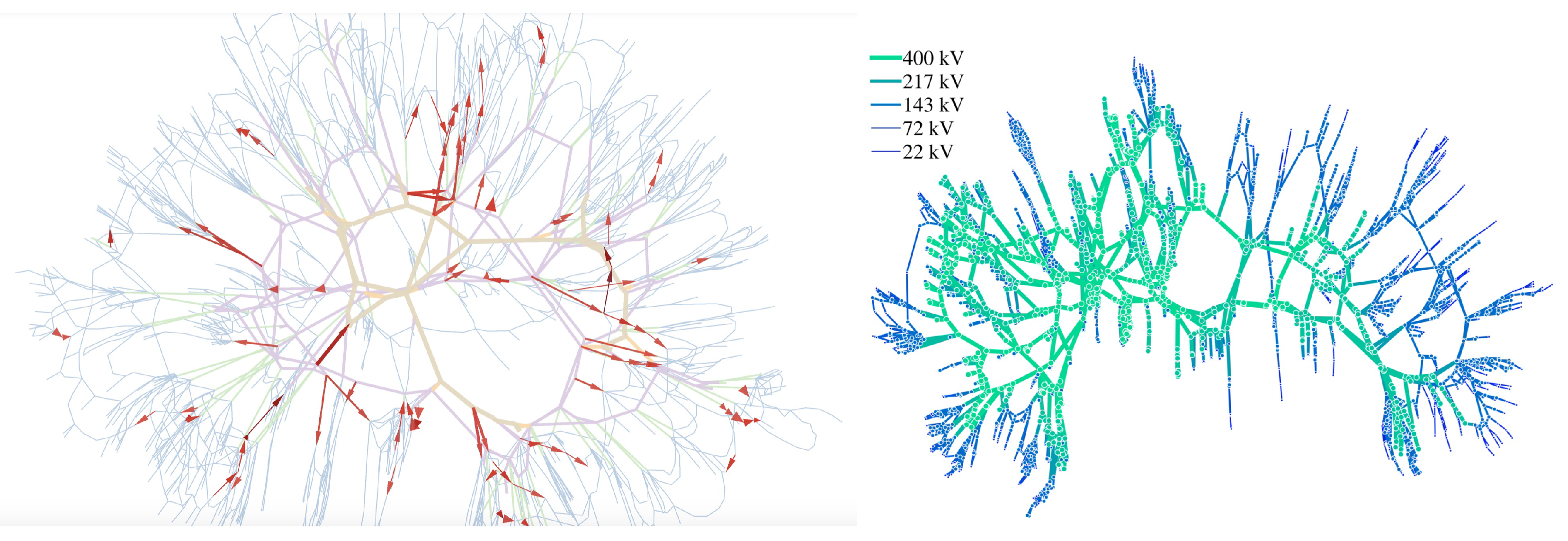
Figure 1. On the left: The red arrows in this network diagram indicate where overloading of power lines could occur in the case2382wp power system, due to short-term fluctuations in (notionally) renewable generator outputs. On the right: The diagram shows the nesta case2224 edin test power system, see [1,2].
Symmetry 11 00136 g001
Figure 2. A comparison between the l 1 norm, the Huber & the pseudo–Huber function, and the l 1 norm & pseudo–Huber function for different values of μ ; see [15,16].
Symmetry 11 00136 g002