Article

Power Spectrum and Diffusion of the Amari Neural Field

1
Dipartimento di Fisica e Astronomia “Galileo Galilei” and CNISM, Università di Padova, Via Marzolo 8, 35131 Padova, Italy
2
Istituto Nazionale di Ottica (INO) del Consiglio Nazionale delle Ricerche (CNR), Via Nello Carrara 1, I-50019 Sesto Fiorentino, Italy
Symmetry 2019, 11(2), 134; https://doi.org/10.3390/sym11020134
Submission received: 29 December 2018 / Revised: 21 January 2019 / Accepted: 22 January 2019 / Published: 26 January 2019

Abstract

:
We study the power spectrum of a space-time dependent neural field which describes the average membrane potential of neurons in a single layer. This neural field is modelled by a dissipative integro-differential equation, the so-called Amari equation. By considering a small perturbation with respect to a stationary and uniform configuration of the neural field we derive a linearized equation which is solved for a generic external stimulus by using the Fourier transform into wavevector-freqency domain, finding an analytical formula for the power spectrum of the neural field. In addition, after proving that for large wavelengths the linearized Amari equation is equivalent to a diffusion equation which admits space-time dependent analytical solutions, we take into account the nonlinearity of the Amari equation. We find that for large wavelengths a weak nonlinearity in the Amari equation gives rise to a reaction-diffusion equation which can be formally derived from a neural action functional by introducing a dual neural field. For some initial conditions, we discuss analytical solutions of this reaction-diffusion equation.

1. Introduction

Neural field theory is the set of models of brain organization and function in which the interaction of billions of neurons is treated as a continuum [1,2]. It was Wilson and Cowan [3], Nunez [4], and Amari [5] in the 1970s who provided the formulations for neural field models that are in common use today [2].
In this paper we analyze one of the most used formulations of neural field activity: The deterministic Amari’s equation [5], which describes the local activity of a population of neurons in a single-layer. We linearize the Amari equation and Fourier-transform it from the space-time domain to the wavevector-freqency domain. In this way we obtain an elegant analytical solution of the equation and, in particular, we determine the power spectrum of the neural field in the case of an instantaneous and localized external stimulus. In the regime of large frequency we show that the power spectrum scales as 1 / ω 2 , which is indeeed a direct consequence of the exponential decay in the time domain. The same 1 / ω 2 law has been obtained [6,7] investigating the stochastic version of the Wilson-Cowan neural field theory [7]. This result is also consistent with the scaling laws found in measurements of electroencephalography (EEG) [8]. Clearly, EEG spectra of intact functional brains are quite complex, showing very prominent resonances (alpha, beta, etc) beyond the 1 / ω 2 shoulder [9]. Modelling these resonances is one of the central issue of theoretical neuroscience [10].
In addition, in this paper we find that for small wavenumbers the Fourier antitransform of the linearized Amari equation gives a diffusion equation, which is thus reliable for large wavelengths. Finally, we investigate some consequences of nonlinearity in the Amari equation. For large wavelengths and weak nonlinearity we deduce a reaction-diffusion equation and discuss some of its spatially uniform solutions. We show that this diffusion equation can be obtained by extremizing a neural action functional by introducing a dual neural field. This action functional is very similar to a neural action recently obtained [7] within a stochastic extension of the Wilson-Cowan model.

2. Amari Equation

The Amari equation [5] is given by
τ t u ( r , t ) = u ( r , t ) + d d r w ( r , r ) f [ u ( r , t ) ] + s ( r , t ) ,
where u ( r , t ) is the space-time dependent neural field, i.e., the average membrane potential of neurons at the position r and time t. Usually d = 3 but often one works with d = 1 or d = 2 [1,2]. Here τ is the (constant) decay time of the one-layer membrane of neurons, w ( r , r ) is the synaptic connection weight from a position r to another position r . We assume that the connections are simmetric
w ( r , r ) = w ( | r r | ) .
The nonlinear function f [ u ] is the activation function usually modelled as a sigmoid, i.e., a Fermi-Dirac distribution
f [ u ] = 1 e β ( h u ) + 1
with gain β > 0 and threshold h > 0 . Finally, s ( r , t ) is an external stimulus acting on neurons [1,2,5].
Let us suppose that the exteral stimulus is absent, i.e., s ( r , t ) = 0 . It is clear from Equation (2) that a stationary and uniform configuration u 0 of the neural field u ( r , t ) satisfies the nonlinear algebric equation
u 0 = W f [ u 0 ] ,
where
W = d d r w ( | r | ) .
If u 0 h from Equation (3) one finds f [ u 0 ] 0 and consequently from Equation (4) it follows u 0 0 . Instead, if u 0 h from Equation (3) one finds f [ u 0 ] 1 and consequently from Equation (4) it follows u 0 W if W > h or u 0 0 if W < h .

3. Linearized Amari Equation

We now consider a perturbation η ( r , t ) with respect to the configuration u 0 of the neural field, namely
u ( r , t ) = u 0 + η ( r , t ) .
If the neural perturbation is sufficiently small, i.e., | η ( r , t ) | u 0 , we can write
f [ u ( r , t ) ] f [ u 0 ] + f [ u 0 ] η ( r , t )
and Equation (2) gives
τ t η ( r , t ) = η ( r , t ) + f [ u 0 ] d d r w ( | r r | ) η ( r , t )
taking into account Equations (4) and (7). This is the linearized Amari’s equation around a uniform and constant configuration u 0 .

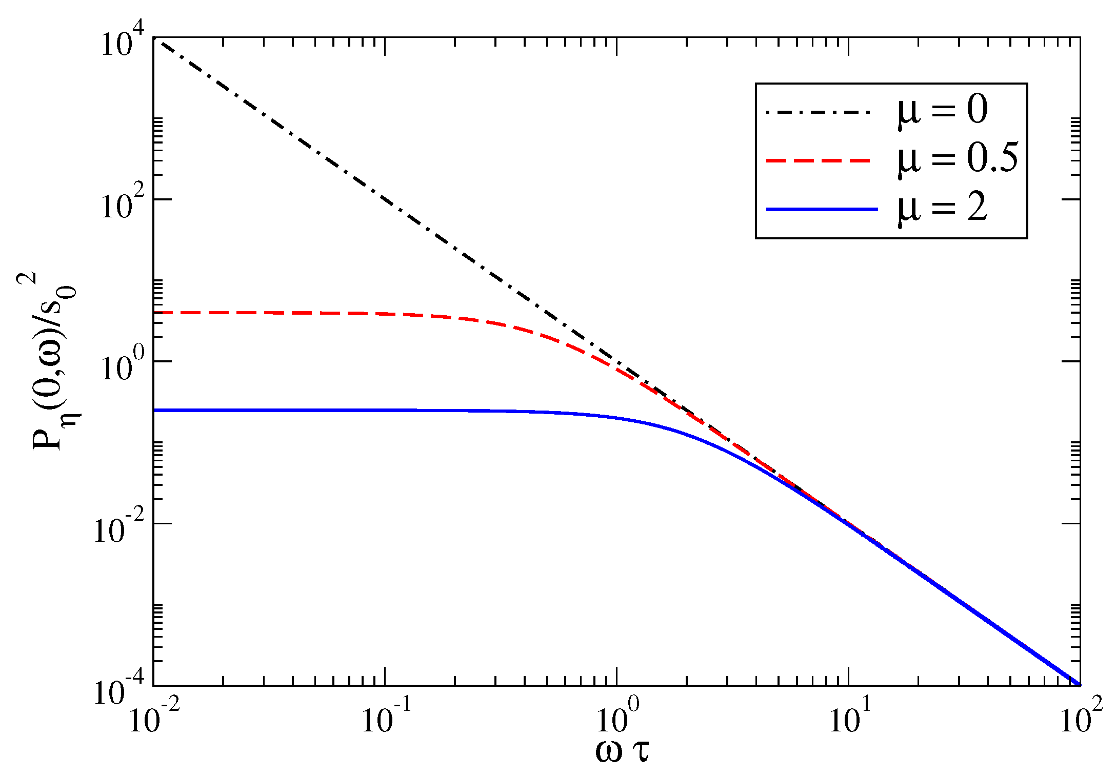
3.1. Power Spectrum of the Linearized Amari Equation

Equation (8) can be transformed into an algebric equation by introducing the Fourier transform [11]
η ˜ ( k , ω ) = F [ η ( r , t ) ] ( k , ω )
where
F [ η ( r , t ) ] ( k , ω ) = d d r d t η ( r , t ) e i ( k · r ω t ) ,
with k the wavevector and ω the frequency and, by definition,
η ( r , t ) = 1 ( 2 π ) d + 1 d d k d ω η ˜ ( k , ω ) e i ( k · r ω t ) .
In fact, by appling the Fourier transform F to Equation (8) and using the properties of F with respect to derivatives and integrals (convolution theorem) one immediately finds
i ω τ + 1 f [ u 0 ] w ˜ ( k ) η ˜ ( k , ω ) = 0 ,
with k = | k | . From this equation the dispersion relation ω = ω k between ω and k reads
ω k = i τ 1 + f [ u 0 ] w ˜ ( k ) .
We stress that Equation (12) can be rewritten as
G 0 1 η ˜ ( k , ω ) = 0 ,
where
G 0 = 1 i ω τ + 1 f [ u 0 ] w ˜ ( k )
is the Green function of the linearized Amari’s equation.
Let us switch on the external stimulus, i.e., s ( r , t ) 0 . The corresponding linearized Amari’s equation in reciprocal wavevector-frequency domain becomes
G 0 1 η ˜ ( k , ω ) = s ˜ ( k , ω )
from which we get the solution
η ˜ ( k , ω ) = G 0 s ˜ ( k , ω )
namely
η ˜ ( k , ω ) = s ˜ ( k , ω ) i ω τ + 1 f [ u 0 ] w ˜ ( k ) .
The power spectrum P η ( k , ω ) of the neural perturbation η ( k , t ) is defined as
P η ( k , ω ) = | η ˜ ( k , ω ) | 2
and taking into account Equation (18) it is given by
P η ( k , ω ) = | s ˜ ( k , ω ) | 2 ω 2 τ 2 + 1 f [ u 0 ] w ˜ ( k ) 2
This simple but elegant analytical formula gives immediately the power spectrum of the neutral field knowing the Fourier transform s ˜ ( k , ω ) of the external stimulus s ( k , t ) .
In the case of an instantaneous stimulus of amplitude s 0 localized at position r = 0 and time t = 0 , i.e.,
s ( r , t ) = s 0 δ ( d ) ( r ) δ ( t ) ,
with δ ( d ) ( r ) the Dirac delta function in d dimensions, the power spectrum of the neural perturbation becomes
P η ( k , ω ) = s 0 2 ω 2 τ 2 + 1 f [ u 0 ] w ˜ ( k ) 2 .
In Figure 1 we plot the power spectrum at k = 0 , i.e.,
P η ( 0 , ω ) = s 0 2 ω 2 τ 2 + μ 2 ,
as a function of the frequency ω in the case of the instantaneous and localized stimulus for three values of the parameter
μ = 1 f [ u 0 ] w ˜ ( 0 ) .
The figure clearly shows that for large frequencies ( ω μ / τ ) the power spectrum is described by the power law
P η ( 0 , ω ) s 0 2 τ 2 1 ω 2 .
As previously discussed, this result, that is valid in the regime of small wavenumbers ( k 0 ), is consistent with the scaling laws found in measurements of electroencephalography (EEG) [8]. It is important to stress that, as written also in the introduction, EEG spectra are quite complex and display clear resonances (alpha, beta, etc.) beyond the 1 / ω 2 shoulder [9]. These nontrivial features can be captured by the inclusion of a time delay in the Amari equation [10,12].
The 1 / ω 2 power-law of the Amari equation, which is mapped into the Wilson-Cowan equation [1], is not surprising. In fact, the exponential decay ( μ > 0 ) in the time domain, i.e.,
η ( t ) = η ( 0 ) e μ t / τ
and consequently
u ( t ) = u 0 + η ( 0 ) e μ t / τ ,
implies a Lorentzian power spectrum in the frequency domain [11]. Note that Equation (27) means that u 0 , which satisfies Equation (4), is a stable fixed point of the uniform Amari equation
τ t u ( t ) = u ( t ) + W f [ u ( t ) ]
under the condition μ = 1 f [ u 0 ] w ˜ ( 0 ) > 0 .

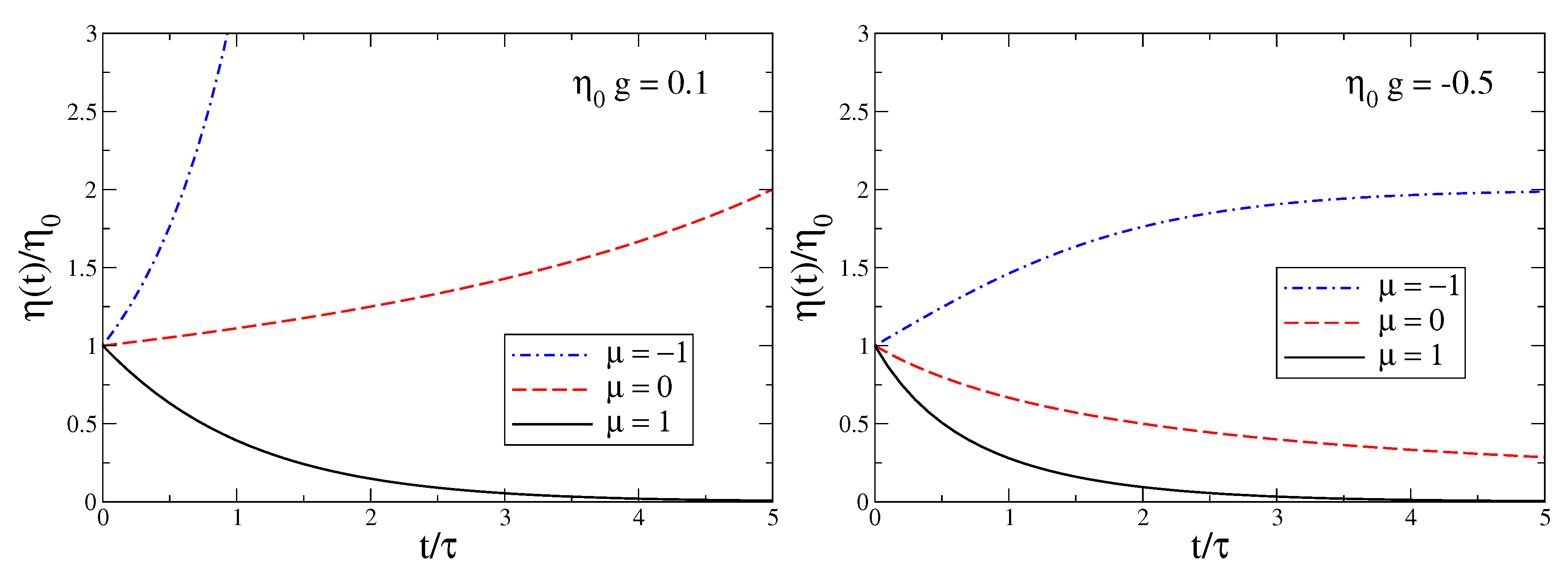
3.2. Diffusion Equation From the Linearized Amari Equation

It is interesting to observe that for small wavenumbers k we can write
w ˜ ( k ) w ˜ ( 0 ) + 1 2 w ˜ ( 0 ) k 2
and the linearized Amari Equation (12) becomes
i ω τ + 1 f [ u 0 ] w ( 0 ) 1 2 f [ u 0 ] w ( 0 ) k 2 η ˜ ( k , ω ) = 0 .
Performing the Fourier antitransform [11] of this equation we obtain
τ t η ( r , t ) = D 2 μ η ( r , t ) ,
with μ = 1 f [ u 0 ] w ˜ ( 0 ) and D = f [ u 0 ] w ˜ ( 0 ) / 2 . Equation (31) is a diffusion equation with D > 0 the diffusion coefficient, which can also be formally interpreted as a time-dependent Schrödinger equation with imaginary time [13], and it is clearly reliable only for large wavelengths λ = 2 π / k . It is well known the Equation (31) admits meaningful analytical solutions [13]. For instance, given the Gaussian initial condition
η ( r , 0 ) = η 0 e r 2 σ 2
induced by some stimulus, the time-dependent solution of Equation (31) reads
η ( r , t ) = η 0 ζ ( t ) d / 2 e r 2 σ 2 ζ ( t ) e μ t / τ
with
ζ ( t ) = 1 + 2 D σ 2 τ t ,
and consequently
u ( r , t ) = u 0 + η 0 ζ ( t ) d / 2 e μ t / τ e r 2 σ 2 ζ ( t )
is a solution of the Amari Equation (2) under the conditions η 0 u 0 (small perturbation) and σ D (large wavelengths).

4. Reaction-Diffusion From the Amari Equation with Weak Nonlinearity

Let us now consider the effect of a weak nonlinearity in the Amari equation. In particular, in the expansion of Equation (7) we add a quadratic term, namely
f [ u ( r , t ) ] f [ u 0 ] + f [ u 0 ] η ( r , t ) + 1 2 f [ u 0 ] η ( r , t ) 2 .
Taking into account also the small wavenumber (long wavelength) expansion of Equation (29) we immediately find a nonlinear reaction-diffusion equation
τ t η ( r , t ) = D 2 μ η ( r , t ) + g η ( r , t ) 2 ,
with g = f [ u 0 ] w ˜ ( 0 ) and neglecting the term proportional to f [ u 0 ] w ˜ ( 0 ) / 4 that is at the second order in both k and η .
It is well known that reaction-diffusion equations admit several kind of solutions: traveling waves, stripes, and dissipative solitons [13]. Here we consider the case of uniform initial perturbation η ( r , 0 ) = η 0 such that the time-dependent but spatially uniform solution η ( t ) of Equation (37) can be obtained from
τ t η ( t ) = μ η ( t ) + g η ( t ) 2 .
By using separation of variables and integration from Equation (38) we obtain the solution
η ( t ) = η 0 e μ t / τ 1 + η 0 g μ e μ t / τ 1 ,
In the special case μ = 0 the uniform solution is
η ( t ) = η 0 1 η 0 g τ t .
The time evolution of η ( t ) is shown for three values of μ in Figure 2. The upper panel of Figure 2 clearly shows that, chosing η 0 g = 0.1 , for μ = 1 there is an exponential decay to zero, for μ = 0 there is a polynomial growth, and for μ = 1 an exponential growth. Actually, for η 0 g > 0 it follows that η ( t ) diverges at t = τ / ( η 0 g ) for μ = 0 and at t = ( τ / | μ | ) ln ( 1 + ( | μ | / ( η 0 g ) ) ) for μ < 0 . Obviously, Equation (31) is valid if the perturbation η ( r , t ) is small, thus a solution makes sense only perturbatively and Equations (39) and (40) can be trusted only for | η ( t ) | | u 0 | . However, if η 0 g < 0 there are no divergences: For μ > 0 there is an exponential decay to zero, for μ = 0 there is polynomial decay to zero, and for μ < 0 one finds η ( t ) μ / g as t . These trends are explicitly shown in the lower panel of Figure 2.

Dissipation and Neural Action

In this subsection we analyze the dissipative nature of Equation (37). Remarkably, dissipative equations can be derived from a variational principle by doubling the degees of freedom [14,15]. Let us show this interesting property by introducing the dual field ϕ ( r , t ) and the neural action functional
S [ η ( r , t ) , ϕ ( r , t ) ] = d d r d t L ,
where
L = ϕ ( r , t ) τ t D 2 + μ η ( r , t ) g ϕ ( r , t ) η ( r , t ) 2
is the Lagrangian density of the neural field. It is straightforward to see that the Euler-Lagrange equation
L ϕ = 0
obtained extemizing the neural action (41) with respect to the dual field ϕ ( r , t ) gives exactly Equation (31), while the Euler-Lagrange equation
L η t L ( t η ) · L ( η ) + 2 L ( 2 η ) = 0
obtained extremizing the neural action (41) with respect to the neutral field η ( r , t ) gives the differential equation of the dual field ϕ ( r , t ) , that is
τ t ϕ ( r , t ) = D 2 + μ ϕ ( r , t ) + 2 g η ( r , t ) ϕ ( r , t ) .
Notice that Equation (31) is independend of ϕ ( r , t ) while Equation (45) depends on η ( r , t ) .
The neural action functional (41) with (46) is similar to the renormalized neural action introduced in Ref. [7]) within a stochastic extension of the Wilson-Cowan model. Using our notations the Lagrangian density of Ref. [7] reads
L = ϕ ( r , t ) τ t D 2 + μ η ( r , t ) g ϕ ( r , t ) η ( r , t ) 2 ϕ ( r , t ) 2 η ( r , t ) ,
which clearly gives a quite different reaction-diffusion equation where it appears explicitly the dual field ϕ ( r , t ) that induces a stochastic noise in the dynamics of the neural field η ( r , t ) . As discussed in Ref. [6,7] the Lagrangian density (46) is called Reggeon field theory [16] and it has a directed percolation phase transition when μ = 0 [17], i.e., when one cross the stability region of the uniform configuration (that is dynamically stable only for μ > 0 , see Equation (28)).
In our approach the dual field ϕ ( r , t ) does not influence the deterministic dissipative dynamics of the neural field, given by Equation (37). However, ϕ ( r , t ) is necessary to derive Equation (37) from a variational principle.

5. Conclusions

By analyzing the Amari equation of a neural field we have obtained an analytical formula for its power spectrum under the assumption of a small perturbation around a stationary uniform neural field in the presence of a generic external stimulus. In the case of a istantaneous and localized external stimulus the power spectrum is quite simple and for large frequencies it scales as 1 / ω 2 . It is important to observe that also in [18] there is an explicit derivation of 1 / ω 2 power law for voltage in cable equations, which are diffusion equations with a source term, while in [19] the same power law is derived analytically for large frequencies in a class of integro-differential equation models with various types of local connectivities. In this paper we have also shown that for large wavelengths (small wavenumbers) the linearized Amari equation is equivalent to a diffusion equation, for which we write the space-time dependent analytical solution in the case of a Gaussian initial perturbation. Finally, taking into account quadratic corrections to the linearized Amari equation we have deduced a reaction-diffusion equation, which can be formally derived by extremizing a neural action functional. This neural action is similar to the one proposed in [7] on the basis of a stochastic extension of the Wilson-Cowan model. We have also shown that, for some specific initial conditions, our reaction-diffusion equation admits meaningful spatially uniform analytical solutions.

Funding

This research received no external funding.

Acknowledgments

The author thanks F. Sattin and F. Toigo for useful discussions.

Conflicts of Interest

The author declares no conflict of interest.

References

  1. Bresloff, P.C. Spatiotemporal dynamics of continuum neural fields. J. Phys. A 2012, 45. [Google Scholar] [CrossRef]
  2. Coombes, S.; Graben, P.B.; Rotthast, R.; Wright, J. (Eds.) Neural Fields: Theory and Applications; Springer: Heidelberg, Germany, 2014. [Google Scholar]
  3. Wilson, H.R.; Cowan, J.D. Excitatory and Inhibitory Interactions in Localized Populations of Model Neurons. Biophys. J. 1972, 12, 1–24. [Google Scholar] [CrossRef] [Green Version]
  4. Nunez, P.L. The brain wave equation: A model for the EEG. Math. Biosci. 1974, 21, 279–297. [Google Scholar] [CrossRef]
  5. Amari, S. Dynamics of excitation patterns in lateral-inhibitory neural fields. Biol. Cyber. 1977, 27, 77–87. [Google Scholar] [CrossRef]
  6. Buice, M.A.; Cowan, J.D. Statistical mechanics of the neocortex. Prog. Biophys. Mol. Biol. 2009, 99, 53–86. [Google Scholar] [CrossRef] [PubMed]
  7. Buice, M.A.; Cowan, J.D. Field-theoretic approach to fluctuation effects in neural networks. Phys. Rev. E 2007, 75, 051919. [Google Scholar] [CrossRef] [PubMed]
  8. Freeman, W.J.; Rogers, L.J.; Holmes, M.D.; Silbergeld, D.L.; Cowan, J.D. Field-theoretic approach to fluctuation effects in neural networks. J. Neurosci. Meth. 2000, 95, 111–121. [Google Scholar] [CrossRef]
  9. Rowe, D.L.; Robinson, P.A.; Rennie, C.J. Estimation of neurophysiological parameters from the waking EEG using a biophysical model of brain dynamics. J. Theor. Biol. 2004, 231, 413–433. [Google Scholar] [CrossRef] [PubMed]
  10. Robinson, P.A.; Rennie, C.J.; Rowe, D.L.; O’Connor, S.C.; Gordon, E. Multiscale brain modelling. Philos. Trans. R. Soc. B 2004, 360. [Google Scholar] [CrossRef] [PubMed]
  11. Stein, E.; Shakarchi, R. Fourier Analysis: An Introduction; Princeton University Press: Princeton, NJ, USA, 2003. [Google Scholar]
  12. Jirsa, V.K.; Haken, H. A derivation of a macroscopic field theory of the brain from the quasi-microscopic neural dynamics. Phys. D Nonlinear Phenomena 1997, 99, 503–526. [Google Scholar] [CrossRef]
  13. Sobolev, S.L.; Dawson, E.R.; Broadbent, T.A.A. Partial Differential Equations of Mathematical Physics; Dover: London, UK, 1989. [Google Scholar]
  14. Bateman, H. On Dissipative Systems and Related Variational Principles. Phys. Rev. 1931, 38, 815–819. [Google Scholar] [CrossRef]
  15. Celeghini, E.; Rasetti, M.; Vitiello, G. Quantum dissipation. Ann. Phys. 1992, 215, 156–170. [Google Scholar] [CrossRef]
  16. Gribov, V. A reggeon diagram technique. Sov. Phys. JEPT 1968, 26, 414–423. [Google Scholar]
  17. Cardy, J.; Sugar, R.J. Directed percolation and Reggeon field theory. Phys. A 1980, 13, L423. [Google Scholar] [CrossRef]
  18. Pettersen, K.H.; Linden, H.; Tetzlaff, T.; Einevoll, T. Power Laws from Linear Neuronal Cable Theory: Power Spectral Densities of the Soma Potential, Soma Membrane Current and Single-Neuron Contribution to the EEG. PLoS Comput. Biol. 2014, 10, e1003928. [Google Scholar] [CrossRef] [PubMed] [Green Version]
  19. Jirsa, V. Neural field dynamics with local and global connectivity and time delay. Philos. Trans. R. Soc. A 2009, 367, 1131. [Google Scholar] [CrossRef] [PubMed]
Figure 1. Scaled power spectrum P η ( 0 , ω ) / s 0 2 of the neutral field as a function of the scaled frequency ω τ in the case of an instantaneous and localized stimulus. Three values of the parameter μ = 1 f [ u 0 ] w ˜ ( 0 ) : μ = 0 (dot-dashed line), μ = 0.5 (dashed line), μ = 2 (solid line).
Symmetry 11 00134 g001
Figure 2. Time evolution of the scaled perturbation η ( t ) / η 0 of the neutral field as a function of the scaled time t / τ in the case of a uniform initial perturbation η 0 with respect to a uniform background u 0 . Curves obtained from Equations (39) and (40) with three values of μ : dot-dashed line with μ = 1 , dashed line with μ = 0 , solid line with μ = 1 . Upper panel: η 0 g = 0.1 . Lower panel η 0 g = 0.5 .
Symmetry 11 00134 g002

