Bounds for the Generalized Distance Eigenvalues of a Graph

Abstract

Let G be a simple undirected graph containing n vertices. Assume G is connected. Let $D(G)$ be the distance matrix, $D^L(G)$ be the distance Laplacian, $D^Q(G)$ be the distance signless Laplacian, and $Tr(G)$ be the diagonal matrix of the vertex transmissions, respectively. Furthermore, we denote by $D_{\alpha }(G)$ the generalized distance matrix, i.e., $D_{\alpha }(G)=\alpha Tr(G)+(1-\alpha )D(G)$, where $\alpha \in [0,1]$. In this paper, we establish some new sharp bounds for the generalized distance spectral radius of G, making use of some graph parameters like the order n, the diameter, the minimum degree, the second minimum degree, the transmission degree, the second transmission degree and the parameter $\alpha$, improving some bounds recently given in the literature. We also characterize the extremal graphs attaining these bounds. As an special cases of our results, we will be able to cover some of the bounds recently given in the literature for the case of distance matrix and distance signless Laplacian matrix. We also obtain new bounds for the k-th generalized distance eigenvalue.

1. Introduction

We will consider simple finite graphs in this paper. A (simple) graph is denoted by $G=(V(G),E(G))$, where $V(G)=\{v_1,v_2,\dots ,v_n\}$ represents its vertex set and $E(G)$ represents its edge set. The order of G is the number of vertices represented by $n=|V(G)|$ and its size is the number of edges represented by $m=|E(G)|$. The neighborhood $N(v)$ of a vertex v consists of the set of vertices that are adjacent to it. The degree $d_G(v)$ or simply $d(v)$ is the number of vertices in $N(v)$. In a regular graph, all its vertices have the same degree. Let $d_{uv}$ be the distance between two vertices $u,v\in V(G)$. It is defined as the length of a shortest path. $D(G)={(d_{uv})}_{u,v\in V(G)}$ is called the distance matrix of G. $\overline{G}$ is the complement of the graph G. It has the same vertex set with G but its edge set consists of the edges not present in G. Moreover, the complete graph $K_n$, the complete bipartite graph $K_{s,t}$, the path $P_n$, and the cycle $C_n$ are defined in the conventional way.

The transmission $T{r}_G(v)$ of a vertex v is the sum of the distances from v to all other vertices in G, i.e., $T{r}_G(v)={\displaystyle \sum _{u\in V(G)}}{d}_{uv}.$ A graph G is said to be k-transmission regular if $T{r}_G(v)=k,$ for each $v\in V(G)$. The transmission (also called the Wiener index) of a graph G, denoted by $W(G)$, is the sum of distances between all unordered pairs of vertices in G. We have ${\displaystyle W(G)=\frac{1}{2}{\displaystyle \sum _{v\in V(G)}}T{r}_G(v)}$.

For a vertex $v_i\in V(G)$, $T{r}_G(v_i)$ is also referred to as the transmission degree, or shortly $T{r}_i$. The sequence of transmission degrees $\{T{r}_1,T{r}_2,\dots ,T{r}_n\}$ is the transmission degree sequence of the graph. ${\displaystyle T_i={\displaystyle \sum _{j=1}^n}{d}_{ij}T{r}_j}$ is called the second transmission degree of $v_i$.

Distance matrix and its spectrum has been studied extensively in the literature, see e.g., [6]. Compared to adjacency matrix, distance matrix encapsulates more information such as a wide range of walk-related parameters, which can be applicable in thermodynamic calculations and have some biological applications in terms of molecular characterization. It is known that embedding theory and molecular stability have to do with graph distance matrix.

Almost all results obtained for the distance matrix of trees were extended to the case of weighted trees by Bapat [12] and Bapat et al. [13]. Not only different classes of graphs but the definition of distance matrix has been extended. Indeed, Bapat et al. [14] generalized the concept of the distance matrix to that of q-analogue of the distance matrix. Let $Tr(G)=diag(T{r}_1,T{r}_2,\dots ,T{r}_n)$ be the diagonal matrix of vertex transmissions of G. The works [7,8,9] introduced the distance Laplacian and the distance signless Laplacian matrix for a connected graph G. The matrix $D^L(G)=Tr(G)-D(G)$ is referred to as the distance Laplacian matrix of G, while the matrix $D^Q(G)=Tr(G)+D(G)$ is the distance signless Laplacian matrix of G. Spectral properties of $D(G)$ and $D^Q(G)$ have been extensively studied since then.

Let A be the adjacency matrix and $\mathrm{Deg}(G)=\mathrm{diag}(d_1,d_2,\cdots ,d_n)$ be the degree matrix G. $Q(G)=\mathrm{Deg}(G)+A$ is the signless Laplacian matrix of G. This matrix has been put forth by Cvetkovic in [16] and since then studied extensively by many researchers. For detailed coverage of this research see [17,18,19,20] and the references therein. To digging out the contribution of these summands in $Q(G)$, Nikiforov in [33] proposed to study the $\alpha$-adjacency matrix $A_{\alpha }(G)$ of a graph G given by $A_{\alpha }(G)=\alpha \mathrm{Deg}(G)+(1-\alpha )A$, where $\alpha \in [0,1]$. We see that $A_{\alpha }(G)$ is a convex combination of the matrices A and $\mathrm{Deg}(G)$. Since $A_0(G)=A$ and $2A_{1/2}(G)=Q(G)$, the matrix $A_{\alpha }(G)$ can underpin a unified theory of A and $Q(G)$. Motivated by [33], Cui et al. [15] introduced the convex combinations $D_{\alpha }(G)$ of $Tr(G)$ and $D(G)$. The matrix $D_{\alpha }(G)=\alpha Tr(G)+(1-\alpha )D(G)$, $0\le \alpha \le 1,$ is called generalized distance matrix of G. Therefore the generalized distance matrix can be applied to the study of other less general constructions. This not only gives new results for several matrices simultaneously, but also serves the unification of known theorems.

Since the matrix $D_{\alpha }(G)$ is real and symmetric, its eigenvalues can be arranged as: ${\partial }_1\ge {\partial }_2\ge \cdots \ge {\partial }_n,$ where ${\partial }_1$ is referred to as the generalized distance spectral radius of $G$. For simplicity, $\partial (G)$ is the shorthand for ${\partial }_1(G)$. By the Perron-Frobenius theorem, $\partial (G)$ is unique and it has a unique generalized distance Perron vector, X, which is positive. This is due to the fact that $D_{\alpha }(G)$ is non-negative and irreducible.

A column vector $X={(x_1,x_2,\dots ,x_n)}^T\in {\mathbb{R}}^n$ is a function defined on $V(G)$. We have $X(v_i)=x_i$ for all i. Moreover,

$$X^T{D}_{\alpha }(G)X=\alpha \sum _{i=1}^{n}Tr(v_i)x_i^2+2(1-\alpha )\sum _{1\le i<j\le n}d(v_i,v_j)x_i{x}_j,$$

and $\lambda$ has an eigenvector X if and only if $X\ne \mathbf{0}$ and

$$\lambda x_v=\alpha Tr(v_i)x_i+(1-\alpha )\sum _{j=1}^{n}d(v_i,v_j)x_j.$$

They are often referred to as the $(\lambda ,x)$-eigenequations of G. If $X\in {\mathbb{R}}^n$ has at least one non-negative element and it is normalized, then in the light of the Rayleigh’s principle, it can be seen that

$$\partial (G)\ge X^T{D}_{\alpha }(G)X,$$

where the equality holds if and only if X becomes the generalized distance Perron vector of G.

Spectral graph theory has been an active research field for the past decades, in which for example distance signless Laplacian spectrum has been intensively explored. The work [41] identified the graphs with minimum distance signless Laplacian spectral radius among some special classes of graphs. The unique graphs with minimum and second-minimum distance signless Laplacian spectral radii among all bicyclic graphs of the same order are identified in [40]. In [24], the authors show some bounding inequalities for distance signless Laplacian spectral radius by utilizing vertex transmissions. In [26], chromatic number is used to derive a lower bound for distance signless Laplacian spectral radius. The distance signless Laplacian spectrum has varies connections with other interesting graph topics such as chromatic number [10]; domination and independence numbers [21], Estrada indices [4,5,22,23,34,35,36,38], cospectrality [11,42], multiplicity of the distance (signless) Laplacian eigenvalues [25,29,30] and many more, see e.g., [1,2,3,27,28,32].

The rest of the paper is organized as follows. In Section 2, we obtain some bounds for the generalized distance spectral radius of graphs using the diameter, the order, the minimum degree, the second minimum degree, the transmission degree, the second transmission degree and the parameter $\alpha$. We then characterize the extremal graphs. In Section 3, we are devoted to derive new upper and lower bounds for the k-th generalized distance eigenvalue of the graph G using signless Laplacian eigenvalues and the $\alpha$-adjacency eigenvalues.

2. Bounds on Generalized Distance Spectral Radius

In this section, we obtain bounds for the generalized distance spectral radius, in terms of the diameter, the order, the minimum degree, the second minimum degree, the transmission degree, the second transmission degree and the parameter $\alpha$.

The following lemma can be found in [31].

Lemma 1.

If A is an $n\times n$ non-negative matrix with the spectral radius $\lambda (A)$ and row sums $r_1,r_2,\dots ,r_n$, then

$$\underset{1\le i\le n}{\min }{r}_i\le \lambda (A)\le \underset{1\le i\le n}{\max }{r}_i.$$

Moreover, if A is irreducible, then both of the equalities holds if and only if the row sums of A are all equal.

The following gives an upper bound for $\partial (G)$, in terms of the order n, the diameter d and the minimum degree $\delta$ of the graph G.

Theorem 1.

Let G be a connected graph of order n having diameter d and minimum degree δ. Then

$$\begin{array}{c}\hfill \partial (G)\le dn-\frac{d(d-1)}{2}-1-\delta (d-1),\end{array}$$

(1)

with equality if and only if G is a regular graph with diameter $\le 2$.

Proof. 

First, it is easily seen that,

$$\begin{array}{ccc}\hfill T{r}_p={\displaystyle \sum _{j=1}^n}{d}_{jp}& \le & d_p+2+3+\cdots +(d-1)+d(n-1-d_p-(d-2))\hfill \\ & =& dn-\frac{d(d-1)}{2}-1-d_p(d-1),\mathrm{for}\mathrm{all}p=1,2,\cdots ,n.\hfill \end{array}$$

(2)

Let $T{r}_{max}=\max \{T{r}_G(v_i):1\le i\le n\}$. For a matrix A denote $\lambda (A)$ its largest eigenvalue. We have

$$\begin{array}{ccc}\hfill \partial (G)& =& \lambda \left(\alpha (Tr(G))+(1-\alpha )D(G)\right)\hfill \\ & \le & \alpha \lambda \left(Tr(G)\right)+(1-\alpha )\lambda \left(D(G)\right)\hfill \\ & \le & \alpha T{r}_{max}+(1-\alpha )T{r}_{max}=T{r}_{max}.\hfill \end{array}$$

Applying Equation (2), the inequality follows.

Suppose that G is regular graph with diameter less than or equal to two, then all coordinates of the generalized distance Perron vector of G are equal. If $d=1$, then $G\cong K_n$ and $\partial =n-1$. Thus equality in (1) holds. If $d=2$, we get $\partial (G)=d_i+2(n-1-d_i)=2n-2-d_i$, and the equality in (1) holds. Note that the equality in (1) holds if and only if all coordinates the generalized distance Perron vector are equal, and hence $D_{\alpha }(G)$ has equal row sums.

Conversely, suppose that equality in (1) holds. This will force inequalities above to become equations. Then we get $T{r}_1=T{r}_2=\cdots =T{r}_n=T{r}_{\max },$ hence all the transmissions of the vertices are equal and so G is a transmission regular graph. If $d\ge 3$, then from the above argument, for every vertex $v_i$, there is exactly one vertex $v_j$ with $d_G(v_i,v_j)=2$, and thus $d=3$, and for a vertex $v_s$ of eccentricity 2,

$$\begin{array}{c}\hfill \partial (G)x_s=d_s{x}_s+2(n-1-d_s)x_s=\left(3n-\frac{3(3-1)}{2}-1-d_s(3-1)\right)x_s,\end{array}$$

implying that $d_s=n-2$, giving that $G=P_4$. But the $D_{\alpha }(P_4)$ is not transmission regular graph. Therefore, G turns out to be regular and its diameter can not be greater than 2. □

Taking $\alpha =\frac{1}{2}$ in Theorem 1, we immediately get the following bound for the distance signless Laplacian spectral radius ${\rho }_1^Q(G)$, which was proved recently in [27].

Corollary 1.

([27], Theorem 2.6) Let G be a connected graph of order $n\ge 3$, with minimum degree ${\delta }_1$, second minimum degree ${\delta }_2$ and diameter d. Then

$$\begin{array}{c}\hfill {\rho }_1^Q(G)\le 2dn-d(d-1)-2-({\delta }_1+{\delta }_2)(d-1),\end{array}$$

with equality if and only if G is (transmission) regular graph of diameter $d\le 2$.

Proof. 

As $2D_{\frac{1}{2}}(G)=D^Q(G)$, letting $\delta ={\delta }_1$ in Theorem 1, we have

$$\begin{array}{c}\hfill {\rho }_1^Q(G)=2\partial (G)\le 2dn-d(d-1)-2-2{\delta }_1(d-1)\le 2dn-d(d-1)-2-({\delta }_1+{\delta }_2)(d-1),\end{array}$$

and the result follows. □

Next, the generalized distance spectral radius $\partial (G)$ of a connected graph and its complement is characterized in terms of a Nordhaus-Gaddum type inequality.

Corollary 2.

Let G be a graph of order n, such that both G and its complement $\overline{G}$ are connected. Let δ and Δ be the minimum degree and the maximum degree of $G$, respectively. Then

$$\begin{array}{c}\hfill \partial (G)+\partial (\overline{G})\le 2nk-(t-1)(t+n+\delta -\Delta -1)-2,\end{array}$$

where $k=\max \{d,\overline{d}\},t=\min \{d,\overline{d}\}$ and $d,\overline{d}$ are the diameters of G and $\overline{G},$ respectively.

Proof. 

Let $\overline{\delta }$ denote the minimum degree of $\overline{G}$. Then $\overline{\delta }=n-1-\Delta$, and by Theorem 1, we have

$$\begin{array}{ccc}\hfill \partial (G)+\partial (\overline{G})& \le & dn-\frac{d(d-1)}{2}-1-\delta (d-1)+\overline{d}n-\frac{\overline{d}(\overline{d}-1)}{2}-1-\overline{\delta }(\overline{d}-1)\hfill \\ & =& n(d+\overline{d})-\frac{1}{2}(d(d-1)+\overline{d}(\overline{d}-1))-2-\delta (d-1)-(n-1-\Delta )(\overline{d}-1)\hfill \\ & \le & 2nk-(t-1)(t+n+\delta -\Delta -1)-2.\hfill \end{array}$$

 □

The following gives an upper bound for $\partial (G)$, in terms of the order n, the minimum degree $\delta ={\delta }_1$ and the second minimum degree ${\delta }_2$ of the graph G.

Theorem 2.

Let G be a connected graph of order n having minimum degree ${\delta }_1$ and second minimum degree ${\delta }_2$. Then for $s={\delta }_1+{\delta }_2$, we have

$$\begin{array}{c}\hfill \partial (G)\le \frac{\alpha \mathsf{\Psi }+\sqrt{{\alpha }^2{\mathsf{\Psi }}^2+4(1-2\alpha )\mathsf{\Theta }}}{2},\end{array}$$

(3)

where $\mathsf{\Theta }=\left(dn-\frac{d(d-1)}{2}-1-{\delta }_1(d-1)\right)\left(dn-\frac{d(d-1)}{2}-1-{\delta }_2(d-1)\right)$ and $\mathsf{\Psi }=2dn-d(d-1)-2-s(d-1)$. Also equality holds if and only if G is a regular graph with diameter at most two.

Proof. 

Let $X={(x_1,x_2,\dots ,x_n)}^T$ be the generalized distance Perron vector of graph G and let $x_i=\max \{x_k|k=1,2,\dots ,n\}$ and $x_j={\max }_{k\ne i}\{x_k|k=1,2,\dots ,n\}$. From the ith equation of $D_{\alpha }(G)X=\partial (G)X$, we obtain

$$\begin{array}{c}\hfill \partial x_i=\alpha T{r}_i{x}_i+(1-\alpha ){\displaystyle \sum _{k=1,k\ne i}^n}{d}_{ik}{x}_k\le \alpha T{r}_i{x}_i+(1-\alpha )T{r}_i{x}_j.\end{array}$$

(4)

Similarly, from the jth equation of $D_{\alpha }(G)X=\partial (G)X$, we obtain

$$\begin{array}{c}\hfill \partial x_j=\alpha T{r}_j{x}_j+(1-\alpha ){\displaystyle \sum _{k=1,k\ne j}^n}{d}_{jk}{x}_k\le \alpha T{r}_j{x}_j+(1-\alpha )T{r}_j{x}_i.\end{array}$$

(5)

Now, by (2), we have,

$$\begin{array}{c}\hfill \left(\partial -\alpha \left(dn-\frac{d(d-1)}{2}-1-d_i(d-1)\right)\right)x_i\le (1-\alpha )\left(dn-\frac{d(d-1)}{2}-1-d_i(d-1)\right)x_j\\ \hfill \left(\partial -\alpha \left(dn-\frac{d(d-1)}{2}-1-d_j(d-1)\right)\right)x_j\le (1-\alpha )\left(dn-\frac{d(d-1)}{2}-1-d_j(d-1)\right)x_i.\end{array}$$

Multiplying the corresponding sides of these inequalities and using the fact that $x_k>0$ for all k, we obtain

$$\begin{array}{c}\hfill {\partial }^2-\alpha (2dn-d(d-1)-2-(d-1)(d_i+d_j))\partial -(1-2\alpha ){\xi }_i{\xi }_j\le 0,\end{array}$$

where ${\xi }_l=dn-\frac{d(d-1)}{2}-1-d_l(d-1)$, $l=i,j$, which in turn gives

$$\begin{array}{c}\hfill \partial (G)\le \frac{\alpha (2dn-d(d-1)-2-s(d-1))+\sqrt{{\alpha }^2{(2dn-d(d-1)-2-s(d-1))}^2+4(1-2\alpha )\mathsf{\Theta }}}{2}.\end{array}$$

Now, using $d_i+d_j\ge {\delta }_1+{\delta }_2$, the result follows.

Suppose that equality occurs in (3), then equality occurs in each of the above inequalities. If equality occurs in (4) and (5), the we obtain $x_i=x_k$, for all $k=1,2,\cdots ,n$ giving that G is a transmission regular graph. Also, equality in (2), similar to that of Theorem 1, gives that G is a graph of diameter at most two and equality in $d_i+d_j\ge {\delta }_1+{\delta }_2$ gives that G is a regular graph. Combining all these it follows that equality occurs in (3) if G is a regular graph of diameter at most two.

Conversely, if G is a connected $\delta$-regular graph of diameter at most two, then $\partial (G)=T{r}_i=dn-\frac{d(d-1)}{2}-1-d_i(d-1)$. Also

$$\begin{array}{cc}& \frac{\alpha (2dn-d(d-1)-2-s(d-1))+\sqrt{{\alpha }^2{(2dn-d(d-1)-2-s(d-1))}^2+4(1-2\alpha )\mathsf{\Theta }}}{2}\hfill \\ =& \frac{\alpha (2dn-d(d-1)-2-s(d-1))+(2dn-d(d-1)-2-s(d-1))(1-\alpha )}{2}\hfill \\ =& dn-\frac{d(d-1)}{2}-1-\delta (d-1)=\partial (G).\hfill \end{array}$$

That completes the proof. □

Remark 1.

For any connected graph G of order n having minimum degree δ, the upper bound given by Theorem 2 is better than the upper bound given by Theorem 1. As

$$\begin{array}{cc}& \frac{\alpha (2dn-d(d-1)-2-s(d-1))+\sqrt{{\alpha }^2{(2dn-d(d-1)-2-s(d-1))}^2+4(1-2\alpha )\mathsf{\Theta }}}{2},\hfill \\ \le & \frac{\alpha (2dn-d(d-1)-2-2\delta (d-1))+\sqrt{{\alpha }^2{(2dn-d(d-1)-2-2\delta (d-1))}^2+4(1-2\alpha )\mathsf{\Phi }}}{2},\hfill \\ =& \frac{\alpha (2dn-d(d-1)-2-2\delta (d-1))+(2dn-d(d-1)-2-2\delta (d-1))(1-\alpha )}{2}\hfill \\ =& dn-\frac{d(d-1)}{2}-1-\delta (d-1),\hfill \end{array}$$

where $\mathsf{\Phi }={(2dn-d(d-1)-2-2\delta (d-1))}^2.$

The following gives an upper bound for $\partial (G)$ by using quantities like transmission degrees as well as second transmission degrees.

Theorem 3.

If the transmission degree sequence and the second transmission degree sequence of G are $\{T{r}_1,T{r}_2,\dots ,T{r}_n\}$ and $\{T_1,T_2,\dots ,T_n\},$ respectively, then

$$\begin{array}{c}\hfill {\displaystyle \partial (G)\le \underset{1\le i\le n}{\max }\left\{\frac{-\beta +\sqrt{{\beta }^2+4(\alpha T{r}_i^2+(1-\alpha )T_i+\beta T{r}_i)}}{2}\right\},}\end{array}$$

(6)

where $\beta \ge 0$ is an unknown parameter. Equality occurs if and only if G is a transmission regular graph.

Proof. 

Let $X=(x_1,\dots ,x_n)$ be the generalized distance Perron vector of G and $x_i=\max \{x_j|j=1,2,\dots ,n\}.$ Since

$$\begin{array}{ccc}\hfill \partial {(G)}^{2}X& =& {(D_{\alpha }(G))}^{2}X={(\alpha Tr+(1-\alpha )D)}^{2}X\hfill \\ & =& {\alpha }^{2}T{r}^{2}X+\alpha (1-\alpha )TrDX+\alpha (1-\alpha )DTrX+{(1-\alpha )}^2{D}^{2}X,\hfill \end{array}$$

we have

$$\begin{array}{c}\hfill {\partial }^2(G)x_i={\alpha }^{2}T{r}_i^2{x}_i+\alpha (1-\alpha )T{r}_i{\displaystyle \sum _{j=1}^n}{d}_{ij}{x}_j+\alpha (1-\alpha ){\displaystyle \sum _{j=1}^n}{d}_{ij}T{r}_j{x}_j+{(1-\alpha )}^2{\displaystyle \sum _{j=1}^n}{\displaystyle \sum _{k=1}^n}{d}_{ij}{d}_{jk}{x}_k.\end{array}$$

Now, we consider a simple quadratic function of $\partial (G):$

$$\begin{array}{ccc}\hfill ({\partial }^2(G)+\beta \partial (G))X& =& ({\alpha }^{2}T{r}^{2}X+\alpha (1-\alpha )TrDX+\alpha (1-\alpha )DTrX+{(1-\alpha )}^2{D}^{2}X)\hfill \\ & +& \beta (\alpha TrX+(1-\alpha )DX).\hfill \end{array}$$

Considering the ith equation, we have

$$\begin{array}{ccc}\hfill ({\partial }^2(G)+\beta \partial (G))x_i& =& {\alpha }^{2}T{r}_i^2{x}_i+\alpha (1-\alpha )T{r}_i{\displaystyle \sum _{j=1}^n}{d}_{ij}{x}_j+\alpha (1-\alpha ){\displaystyle \sum _{j=1}^n}{d}_{ij}T{r}_j{x}_j\hfill \\ & +& {(1-\alpha )}^2{\displaystyle \sum _{j=1}^n}{\displaystyle \sum _{k=1}^n}{d}_{ij}{d}_{jk}{x}_k+\beta \left(\alpha T{r}_i{x}_i+\alpha (1-\alpha ){\displaystyle \sum _{j=1}^n}{d}_{ij}{x}_j\right).\hfill \end{array}$$

It is easy to see that the inequalities below are true

$${\displaystyle \alpha (1-\alpha )T{r}_i\sum _{j=1}^n{d}_{ij}{x}_j\le \alpha (1-\alpha )T{r}_i^2{x}_i,\alpha (1-\alpha )\sum _{j=1}^n{d}_{ij}T{r}_j{x}_j\le \alpha (1-\alpha )T_i{x}_i,}$$

$${\displaystyle {(1-\alpha )}^2\sum _{j=1}^n\sum _{k=1}^n{d}_{jk}{d}_{ij}{x}_k\le {(1-\alpha )}^2{T}_i{x}_i,(1-\alpha )\sum _{j=1}^n{d}_{ij}{x}_j\le (1-\alpha )T{r}_i{x}_i.}$$

Hence, we have

$$\begin{array}{c}({\partial }^2(G)+\beta \partial (G))x_i\le \alpha T{r}_i^2{x}_i-\alpha T_i{x}_i+T_i{x}_i+\beta T{r}_i{x}_i\hfill \\ \Rightarrow {\partial }^2(G)+\beta \partial (G)-(\alpha T{r}_i^2-(\alpha -1)T_i+\beta T{r}_i)\le 0\hfill \\ \Rightarrow \partial (G)\le \frac{-\beta +\sqrt{{\beta }^2+4(\alpha T{r}_i^2-(\alpha -1)T_i+\beta T{r}_i)}}{2}.\hfill \end{array}$$

From this the result follows.

Now, suppose that equality occurs in (6), then each of the above inequalities in the above argument occur as equalities. Since each of the inequalities

$$\begin{array}{c}{\displaystyle \alpha (1-\alpha )T{r}_i\sum _{j=1}^n{d}_{ij}{x}_j\le \alpha (1-\alpha )T{r}_i^2{x}_i,\alpha (1-\alpha )\sum _{j=1}^n{d}_{ij}T{r}_j{x}_j\le \alpha (1-\alpha )T_i{x}_i}\hfill \end{array}$$

and

$$\begin{array}{c}\hfill {\displaystyle {(1-\alpha )}^2\sum _{j=1}^n\sum _{k=1}^n{d}_{jk}{d}_{ij}{x}_k\le {(1-\alpha )}^2{T}_i{x}_i,(1-\alpha )\sum _{j=1}^n{d}_{ij}{x}_j\le (1-\alpha )T{r}_i{x}_i,}\end{array}$$

occur as equalities if and only if G is a transmission regular graph. It follows that equality occurs in (6) if and only if G is a transmission regular graph. That completes the proof. □

The following upper bound for the generalized distance spectral radius $\partial (G)$ was obtained in [15]:

$$\begin{array}{c}\hfill {\displaystyle \partial (G)\le \underset{1\le i\le n}{\max }\left\{\sqrt{\alpha T{r}_i^2+(1-\alpha )T_i}\right\},}\end{array}$$

(7)

with equality if and only if $\alpha T{r}_i^2+(1-\alpha )T_i$ is same for i.

Remark 2.

For a connected graph G having transmission degree sequence $\{T{r}_1,T{r}_2,\dots ,T{r}_n\}$ and the second transmission degree sequence $\{T_1,T_2,\dots ,T_n\}$, provided that $T_i\le T{r}_i^2$ for all i, we have

$$\begin{array}{c}\frac{-\beta +\sqrt{{\beta }^2+4\alpha T{r}_i^2+4(1-\alpha )T_i+4\beta T{r}_i}}{2}\le \sqrt{\alpha T{r}_i^2+(1-\alpha )T_i}.\hfill \end{array}$$

Therefore, the upper bound given by Theorem 3 is better than the upper bound given by (7).

If, in particular we take the parameter $\beta$ in Theorem 3 equal to the vertex covering number $\tau$, the edge covering number, the clique number $\omega$, the independence number, the domination number, the generalized distance rank, minimum transmission degree, maximum transmission degree, etc., then Theorem 3 gives an upper bound for $\partial (G)$, in terms of the vertex covering number $\tau$, the edge covering number, the clique number $\omega$, the independence number, the domination number, the generalized distance rank, minimum transmission degree, maximum transmission degree, etc.

Let $x_i=\min \{x_j|j=1,2,\dots ,n\}$ be the minimum among the entries of the generalized distance Perron vector $X=(x_1,\dots ,x_n)$ of the graph G. Proceeding similar to Theorem 3, we obtain the following lower bound for $\partial (G)$, in terms of the transmission degrees, the second transmission degrees and a parameter $\beta$.

Theorem 4.

If the transmission degree sequence and the second transmission degree sequence of G are $\{T{r}_1,T{r}_2,\dots ,T{r}_n\}$ and $\{T_1,T_2,\dots ,T_n\}$, respectively, then

$$\begin{array}{c}\hfill {\displaystyle \partial (G)\ge \underset{1\le i\le n}{\min }\left\{\frac{-\beta +\sqrt{{\beta }^2+4(\alpha T{r}_i^2+(1-\alpha )T_i+\beta T{r}_i)}}{2}\right\},}\end{array}$$

where $\beta \ge 0$ is an unknown parameter. Equality occurs if and only if G is a transmission regular graph.

Proof. 

Similar to the proof of Theorem 3 and is omitted. □

The following lower bound for the generalized distance spectral radius was obtained in [15]:

$$\begin{array}{c}\hfill {\displaystyle \partial (G)\ge \underset{1\le i\le n}{\min }\left\{\sqrt{\alpha T{r}_i^2+(1-\alpha )T_i}\right\},}\end{array}$$

(8)

with equality if and only if $\alpha T{r}_i^2+(1-\alpha )T_i$ is same for i.

Similar to Remark 2, it can be seen that the lower bound given by Theorem 4 is better than the lower bound given by (8) for all graphs G with $T_i\ge T{r}_i^2$, for all i.

Again, if in particular we take the parameter $\beta$ in Theorem 4 equal to the vertex covering number $\tau$, the edge covering number, the clique number $\omega$, the independence number, the domination number, the generalized distance rank, minimum transmission degree, maximum transmission degree, etc, then Theorem 4 gives a lower bound for $\partial (G)$, in terms of the vertex covering number $\tau$, the edge covering number, the clique number $\omega$, the independence number, the domination number, the generalized distance rank, minimum transmission degree, maximum transmission degree, etc.

$G_1\nabla G_2$ is referred to as join of $G_1$ and $G_2$. It is defined by joining every vertex in $G_1$ to every vertex in $G_2$.

Example 1.

(a) Let $C_4$ be the cycle of order 4. One can easily see that $C_4$ is a 4-transmission regular graph and the generalized distance spectrum of $C_4$ is $\{4,4\alpha ,6\alpha -2^{\left[2\right]}\}$. Hence, $\partial (C_4)=4$. Moreover, the transmission degree sequence and the second transmission degree sequence of $C_4$ are $\{4,4,4,4\}$ and $\{16,16,16,16\}$, respectively. Now, putting $\beta =T{r}_{max}=4$ in the given bound of Theorem 3, we can see that the equality holds:

$$\partial (C_4)\le \frac{-4+\sqrt{16+4(16\alpha +16(1-\alpha )+16)}}{2}=\frac{-4+\sqrt{144}}{2}=4.$$

(b) Let $W_{n+1}$ be the wheel graph of order $n+1$. It is well known that $W_{n+1}=C_n\nabla K_1.$ The distance signless Laplacian matrix of $W_5$ is

$$D^Q(W_5)=\left(\begin{array}{ccccc}5& 1& 2& 1& 1\\ 1& 5& 1& 2& 1\\ 2& 1& 5& 1& 1\\ 1& 2& 1& 5& 1\\ 1& 1& 1& 1& 4\end{array}\right).$$

Hence the distance signless Laplacian spectrum of $W_5$ is $spec(W_5)=\left\{\frac{13+\sqrt{41}}{4},\frac{13-\sqrt{41}}{4},\frac{5}{2},{\frac{3}{2}}^{\left[2\right]}\right\}$, and then the distance signless Laplacian spectral radius is ${\rho }_1^Q(W_5)=\frac{13+\sqrt{41}}{4}$. Also, the transmission degree sequence and the second transmission degree sequence of $W_5$ are $\{5,5,5,5,4\}$ and $\{24,24,24,24,20\}$, respectively. As $D_{\frac{1}{2}}(G)=\frac{1}{2}{D}^Q(G)$, taking $\alpha =\frac{1}{2}$ and $\beta =T{r}_{max}=5$ in the given bound of Theorem 3, we immediately get the following upper bound for the distance signless Laplacian spectral radius ${\rho }_1^Q(W_5)$:

$$\frac{1}{2}{\rho }_1^Q(W_5)\le \frac{-5+\sqrt{25+50+48+100}}{2}=\frac{-5+\sqrt{223}}{2},$$

which implies that

$${\rho }_1^Q(W_5)\le -5+\sqrt{223}\simeq 9.93.$$

3. Bounds for the k-th Generalized Distance Eigenvalue

In this section, we discuss the relationship between the generalized distance eigenvalues and the other graph parameters.

The following lemma can be found in [37].

Lemma 2.

Let X and Y be Hermitian matrices of order n such that $Z=X+Y$, and denote the eigenvalues of a matrix M by ${\lambda }_1\ge {\lambda }_2\ge \cdots \ge {\lambda }_n$.Then

$$\begin{array}{c}\hfill {\lambda }_k(Z)\le {\lambda }_j(X)+{\lambda }_{k-j+1}(Y),n\ge k\ge j\ge 1,\\ \hfill {\lambda }_k(Z)\ge {\lambda }_j(X)+{\lambda }_{k-j+n}(Y),n\ge j\ge k\ge 1,\end{array}$$

where ${\lambda }_i(M)$ is the ith largest eigenvalue of the matrix M. Any equality above holds if and only if a unit vector can be an eigenvector corresponding to each of the three eigenvalues.

The following gives a relation between the generalized distance eigenvalues of the graph G of diameter 2 and the signless Laplacain eigenvalues of the complement $\overline{G}$ of the graph G. It also gives a relation between generalized distance eigenvalues of the graph G of diameter greater than or equal to 3 with the $\alpha$-adjacency eigenvalues of the complement $\overline{G}$ of the graph G.

Theorem 5.

Let G be a connected graph of order $n\ge 4$ having diameter d. Let $\overline{G}$ be the complement of G and let ${\overline{q}}_1\ge {\overline{q}}_2\ge \cdots \ge {\overline{q}}_n$ be the signless Laplacian eigenvalues of $\overline{G}$. If $d=2$, then for all $k=1,2,\cdots ,n$, we have

$$\begin{array}{c}\hfill (3\alpha -1)n-2\alpha +(1-2\alpha )d_k+(1-\alpha ){\overline{q}}_k\le {\partial }_k(G)\le (2n-2)\alpha +(1-2\alpha )d_k+(1-\alpha ){\overline{q}}_k.\end{array}$$

Equality occurs on the right if and only if $k=1$ and G is a transmission regular graph and on the left if and only if $k\ne 1$ and G is a transmission regular graph.

If $d\ge 3$, then for all $k=1,2,\cdots ,n$, we have

$$\begin{array}{c}\hfill \alpha n-1+{\lambda }_k(A_{\alpha }(\overline{G}))+{\lambda }_n(M^{\prime })\le {\partial }_k(G)\le n-1+{\lambda }_k(A_{\alpha }(\overline{G}))+{\lambda }_1(M^{\prime }),\end{array}$$

where $A_{\alpha }(\overline{G})=\alpha \mathrm{Deg}(\overline{G})+(1-\alpha )\overline{A}$ is the α-adjacency matrix of $\overline{G}$ and $M^{\prime }=\alpha T{r}^{\prime }(G)+(1-\alpha )M$ with $M=(m_{ij})$ a symmetric matrix of order n having $m_{ij}=\max \{0,d_{ij}-2\}$, $d_{ij}$ is the distance between the vertices $v_i$, $v_j$ and $T{r}^{\prime }(G)=\mathrm{diag}(T{r}_1^{\prime },T{r}_2^{\prime },\cdots ,T{r}_n^{\prime })$, $T{r}_i^{\prime }={\displaystyle \sum _{d_{ij}\ge 3}}(d_{ij}-2)$.

Proof. 

Let G be a connected graph of order $n\ge 4$ having diameter d. Let $\mathrm{Deg}(\overline{G})=diag(n-1-d_1,n-1-d_2,\cdots ,n-1-d_n)$ be the diagonal matrix of vertex degrees of $\overline{G}$. Suppose that diameter d of G is two, then transmission degree $T{r}_i=2n-2-d_i$, for all $i,$ then the distance matrix of G can be written as $D(G)=A+2\overline{A}$, where A and $\overline{A}$ are the adjacency matrices of G and $\overline{G}$, respectively. We have

$$\begin{array}{cc}\hfill D_{\alpha }(G)& =\alpha Tr(G)+(1-\alpha )D(G)=\alpha (2n-2)I-\alpha \mathrm{Deg}(G)+(1-\alpha )(A+2\overline{A})\hfill \\ & =\alpha (2n-2)I-\alpha \mathrm{Deg}(G)+(1-\alpha )(A+\overline{A})+(1-\alpha )\overline{A}\hfill \\ & =(3n\alpha -n-2\alpha )I+(1-\alpha )J+(1-2\alpha )\mathrm{Deg}(G)+(1-\alpha )Q(\overline{G}),\hfill \end{array}$$

where I is the identity matrix and J is the all one matrix of order n. Taking $Y=(3n\alpha -n-2\alpha )I+(1-2\alpha )\mathrm{Deg}(G)+(1-\alpha )Q(\overline{G})$, $X=(1-\alpha )J$, $j=1$ in the first inequality of Lemma 2 and using the fact that $spec(J)=\{n,0^{[n-1]}\},$ it follows that

$$\begin{array}{c}\hfill {\partial }_k(G)\le (2n-2)\alpha +(1-2\alpha )d_k+(1-\alpha ){\overline{q}}_k,\mathrm{for}\mathrm{all}k=1,2,\cdots ,n.\end{array}$$

(9)

Again, taking $Y=(3n\alpha -n-2\alpha )I+(1-2\alpha )\mathrm{Deg}(G)+(1-\alpha )Q(\overline{G})$, $X=(1-\alpha )J$ and $j=n$ in the second inequality of Lemma 2, it follows that

$$\begin{array}{c}\hfill {\partial }_k(G)\ge (3\alpha -1)n-2\alpha +(1-2\alpha )d_k+(1-\alpha ){\overline{q}}_k,\mathrm{for}\mathrm{all}k=1,2,\cdots ,n.\end{array}$$

(10)

Combining (9) and (10) the first inequality follows. Equality occurs in first inequality if and only if equality occurs in (9) and (10). Suppose that equality occurs in (9), then by Lemma 2, the eigenvalues ${\partial }_k,(3n-2)\alpha -n+(1-2\alpha )d_k+(1-\alpha ){\overline{q}}_k$ and $n(1-\alpha )$ of the matrices $D_{\alpha }(G),X$ and Y have the same unit eigenvector. Since $\mathbf{1}=\frac{1}{n}{(1,1,\cdots ,1)}^T$ is the unit eigenvector of Y for the eigenvalue $n(1-\alpha )$, it follows that equality occurs in (9) if and only if $\mathbf{1}$ is the unit eigenvector for each of the matrices $D_{\alpha }(G),X$ and Y. This gives that G is a transmission regular graph and $\overline{G}$ is a regular graph. Since a graph of diameter 2 is regular if and only if it is transmission regular and complement of a regular graph is regular. Using the fact that for a connected graph G the unit vector $\mathbf{1}$ is an eigenvector for the eigenvalue ${\partial }_1$ if and only if G is transmission regular graph, it follows that equality occurs in first inequality if and only if $k=1$ and G is a transmission regular graph.

Suppose that equality occurs in (10), then again by Lemma 2, the eigenvalues ${\partial }_k,(3n-2)\alpha -n+(1-2\alpha )d_k+(1-\alpha ){\overline{q}}_k$ and 0 of the matrices $D_{\alpha }(G),X$ and Y have the same unit eigenvector $\mathit{x}$. Since $J\mathit{x}=0$, it follows that ${\mathit{x}}^T\mathbf{1}=0$. Using the fact that the matrix J is symmetric(so its normalized eigenvectors are orthogonal [43]), we conclude that the vector $\mathbf{1}$ belongs to the set of eigenvectors of the matrix J and so of the matrices $D_{\alpha }(G),X$. Now, $\mathbf{1}$ is an eigenvector of the matrices $D_{\alpha }(G)$ and X, gives that G is a regular graph. Since for a regular graph of diameter 2 any eigenvector of $Q(\overline{G})$ and $D_{\alpha }(G)$ is orthogonal to $\mathbf{1}$, it follows that equality occurs in (10) if and only if $k\ne 1$ and G is a regular graph.

If $d\ge 3$, we define the matrix $M=(m_{ij})$ of order n, where $m_{ij}=\max \{0,d_{ij}-2\}$, $d_{ij}$ is the distance between the vertices $v_i$ and $v_j$. The transmission of a vertex $v_i$ can be written as $T{r}_i=d_i+2{\overline{d}}_i+T{r}_i^{\prime }$, where $T{r}_i^{\prime }={\displaystyle \sum _{d_{ij}\ge 3}}(d_{ij}-2)$, is the contribution from the vertices which are at distance more than two from $v_i$. For $T{r}^{\prime }(G)=\mathrm{diag}(T{r}_1^{\prime },T{r}_2^{\prime },\cdots ,T{r}_n^{\prime })$, we have

$$\begin{array}{c}{D}_{\alpha }(G)=\alpha Tr(G)+(1-\alpha )D(G)=\alpha \mathrm{Deg}(G)+2\alpha \mathrm{Deg}(\overline{G})+\alpha T{r}^{\prime }(G)+(1-\alpha )(A+2\overline{A}+M)\hfill \\ =\alpha (\mathrm{Deg}(G)+\mathrm{Deg}(\overline{G}))+(1-\alpha )(A+\overline{A})+(\alpha \mathrm{Deg}(\overline{G})+(1-\alpha )\overline{A})+(\alpha T{r}^{\prime }(G)+(1-\alpha )M)\hfill \\ =D_{\alpha }(K_n)+A_{\alpha }(\overline{G})+M^{\prime },\hfill \end{array}$$

where $A_{\alpha }(\overline{G})$ is the $\alpha$-adjacency matrix of $\overline{G}$ and $M^{\prime }=\alpha T{r}^{\prime }(G)+(1-\alpha )M$. Taking $X=D_{\alpha }(K_n)$, $Y=A_{\alpha }(\overline{G})+M^{\prime }$ and $j=1$ in the first inequality of Lemma 2 and using the fact that $spec(D_{\alpha }(K_n))=\{n-1,\alpha n-1^{[n-1]}\},$ it follows that

$$\begin{array}{c}\hfill {\partial }_k(G)\le n-1+{\lambda }_k(A_{\alpha }(\overline{G})+M^{\prime }),\mathrm{for}\mathrm{all}k=1,2,\cdots ,n.\end{array}$$

Again, taking $Y=A_{\alpha }(\overline{G})$, $X=M^{\prime }$ and $j=1$ in the first inequality of Lemma 2, we obtain

$$\begin{array}{c}\hfill {\partial }_k(G)\le n-1+{\lambda }_k(A_{\alpha }(\overline{G}))+{\lambda }_1(M^{\prime }),\mathrm{for}\mathrm{all}k=1,2,\cdots ,n.\end{array}$$

(11)

Similarly, taking $X=D_{\alpha }(K_n)$, $Y=A_{\alpha }(\overline{G})+M^{\prime }$ and $j=n$ and then $Y=A_{\alpha }(\overline{G})$, $X=M^{\prime }$ and $j=n$ in the second inequality of Lemma 2, we obtain

$$\begin{array}{c}\hfill {\partial }_k(G)\ge \alpha n-1+{\lambda }_k(A_{\alpha }(\overline{G}))+{\lambda }_n(M^{\prime }),\mathrm{for}\mathrm{all}k=1,2,\cdots ,n.\end{array}$$

(12)

From (11) and (12) the second inequality follows. That completes the proof. □

It can be seen that the matrix $M^{\prime }$ defined in Theorem 5 is positive semi-definite for all $\frac{1}{2}\le \alpha \le 1$. Therefore, we have the following observation from Theorem 5.

Corollary 3.

Let G be a connected graph of order $n\ge 4$ having diameter $d\ge 3$. If $\frac{1}{2}\le \alpha \le 1$, then

$$\begin{array}{c}\hfill {\partial }_k(G)\ge \alpha n-1+{\lambda }_k(A_{\alpha }(\overline{G})),forallk=1,2,\cdots ,n,\end{array}$$

where $A_{\alpha }(\overline{G})=\alpha \mathrm{Deg}(\overline{G})+(1-\alpha )\overline{A}$ is the α-adjacency matrix of $\overline{G}$.

It is clear from Corollary 3 that for $\frac{1}{2}\le \alpha \le 1$, any lower bound for the $\alpha$-adjacency ${\lambda }_k(A_{\alpha }(\overline{G}))$ gives a lower bound for ${\partial }_k$ and conversely any upper bound for ∂ gives an upper bound for ${\lambda }_k(A_{\alpha }(\overline{G}))$. We note that Theorem 5 generalizes one of the Theorems (namely Theorem 3.8) given in [8].

Example 2.

(a) Let $C_n$ be a cycle of order $n$. It is well known (see [7]) that $C_n$ is a k-transmission regular graph with $k=\frac{n^2}{4}$ if n is even and $k=\frac{n^2-1}{4}$ if n is odd. Let $n=4$. It is clear that the distance spectrum of the graph $C_4$ is $\{4,0,-2^{\left[2\right]}\}$. Also, since $C_4$ is a 4-transmission regular graph, then $Tr(C_4)=4I_4$ and so $D_{\alpha }(C_4)=4\alpha I_4+(1-\alpha )D(C_4)$. Hence the generalized distance spectrum of $C_4$ is $\{4,4\alpha ,6\alpha -2^{\left[2\right]}\}$. Moreover, the signless Laplacian spectrum of $\overline{C_4}$ is $\{2^{\left[2\right]},0^{\left[2\right]}\}$. Since the diameter of $C_4$ is 2, hence, applying Theorem 5, for $k=1$, we have,

$$4\alpha =4(3\alpha -1)-2\alpha +2(1-2\alpha )+2(1-\alpha )\le {\partial }_1(C_4)=4\le 6\alpha +2(1-2\alpha )+2(1-\alpha )=4,$$

which shows that the equality occurs on right for $k=1$ and transmission regular graph $C_4$.

Also, for $k=2$, we have

$$4\alpha =4(3\alpha -1)-2\alpha +2(1-2\alpha )+2(1-\alpha )\le {\partial }_2(C_4)=4\alpha \le 6\alpha +2(1-2\alpha )+2(1-\alpha )=4,$$

which shows that the equality occurs on left for $k=2$ and transmission regular graph $C_4$.

(b) Let $C_6$ be a cycle of order 6. It is clear that the distance spectrum of the graph $C_6$ is $\{9,0^{\left[2\right]},-1,-4^{\left[2\right]}\}$. Since $C_6$ is a 9-transmission regular graph, then $Tr(C_6)=9I_6$ and so $D_{\alpha }(C_6)=9\alpha I_6+(1-\alpha )D(C_6)$. Hence, the generalized distance spectrum of $C_6$ is $\{9,9{\alpha }^{\left[2\right]},10\alpha -1,13\alpha -4^{\left[2\right]}\}$. Also, the α-adjacency spectrum of $C_6$ is $\{3,2\alpha +1,3{\alpha }^{\left[2\right]},5\alpha -2^{\left[2\right]}\}$. Let $M^{\prime }$ be the matrix defined by the Theorem 5, hence the spectrum of $M^{\prime }$ is $\{1^{\left[3\right]},2\alpha -1^{\left[3\right]}\}.$ Since diameter of the graph $C_6$ is 3, hence, applying Theorem 5, for $k=1$, we have

$$8\alpha +1=6\alpha -1+3+2\alpha -1\le {\partial }_1(C_6)=9\le 5+3+1=9.$$

Also for $k=2,$ we have

$$10\alpha -1=6\alpha -1+2\alpha +1+2\alpha -1\le {\partial }_2(C_6)=9\alpha \le 5+2\alpha +1+1=2\alpha +7.$$

We need the following lemma proved by Hoffman and Wielandt [39].

Lemma 3.

Suppose we have $C=A+B$. Here, all these matrices are symmetric and have order n. Suppose they have the eigenvalues ${\alpha }_i,{\beta }_i,$ and ${\gamma }_i,$ where $1\le i\le n,$ respectively arranged in non-increasing order. Therefore, ${\sum }_{i=1}^n{({\gamma }_i-{\alpha }_i)}^2\le {\sum }_{i=1}^n{\beta }_i^2.$

The following gives relation between generalized distance spectrum and distance spectrum for a simple connected graph G. We use $\left[n\right]$ to denote the set of $\{1,2,\dots ,n\}.$ For each subset S of $\left[n\right],$ we use $S^c$ to denote $\left[n\right]-S.$

Theorem 6.

Let G be a connected graph of order n and let ${\mu }_1,\dots ,{\mu }_n$ be the eigenvalues of the distance matrix of $G$. Then for each non-empty subset $S=\{r_1,r_2,\dots ,r_k\}$ of $\left[n\right]$, we have the following inequalities:

$$\begin{array}{cc}& \frac{2k\alpha W(G)-\sqrt{k(n-k)\left(n{\sum }_{i=1}^n{\alpha }^{2}T{r}_i^2-4{\alpha }^2{W}^2(G)\right)}}{n}\hfill \\ \le & {\displaystyle \sum _{i\in S}}({\partial }_i+(\alpha -1){\mu }_i)\hfill \\ \le & \frac{2k\alpha W(G)+\sqrt{k(n-k)\left(n{\sum }_{i=1}^n{\alpha }^{2}T{r}_i^2-4{\alpha }^2{W}^2(G)\right)}}{n}.\hfill \end{array}$$

Proof. 

Since $D_{\alpha }(G)=\alpha Tr(G)+(1-\alpha )D(G)$, then by the fact that $2\alpha W(G)={\sum }_{i=1}^n({\partial }_i+(\alpha -1){\mu }_i),$ we get $2\alpha W(G)-{\sum }_{i\in S}({\partial }_i+(\alpha -1){\mu }_i)={\sum }_{i\in S^C}({\partial }_i+(\alpha -1){\mu }_i).$ By Cauchy-Schwarz inequality, we further have that

$$\begin{array}{c}\hfill {\left(2\alpha W(G)-{\displaystyle \sum _{i\in S}}({\partial }_i+(\alpha -1){\mu }_i)\right)}^2\le {\displaystyle \sum _{i\in S^C}}{1}^2{\displaystyle \sum _{i\in S^C}}{({\partial }_i+(\alpha -1){\mu }_i)}^2.\end{array}$$

Therefore

$$\begin{array}{c}{\left(2\alpha W(G)-{\displaystyle \sum _{i\in S}}({\partial }_i+(\alpha -1){\mu }_i)\right)}^2\hfill \\ \le (n-k)\left({\displaystyle \sum _{i=1}^n}{({\partial }_i+(\alpha -1){\mu }_i)}^2-{\displaystyle \sum _{i\in S}}{({\partial }_i+(\alpha -1){\mu }_i)}^2\right).\hfill \end{array}$$

By Lemma 3, we have that

$$\begin{array}{c}{\left(2\alpha W(G)-{\displaystyle \sum _{i\in S}}({\partial }_i+(\alpha -1){\mu }_i)\right)}^2+(n-k){\displaystyle \sum _{i\in S}}{({\partial }_i+(\alpha -1){\mu }_i)}^2\hfill \\ \le (n-k){\displaystyle \sum _{i=1}^n}{({\partial }_i+(\alpha -1){\mu }_i)}^2\le (n-k){\displaystyle \sum _{i=1}^n}{\alpha }^{2}T{r}_i^2.\hfill \end{array}$$

Again by Cauchy-Schwarz inequality, we have that

$$\begin{array}{cc}& \left(\frac{n-k}{k}\right){\left({\displaystyle \sum _{i\in S}}({\partial }_i+(\alpha -1){\mu }_i)\right)}^2={\left({\displaystyle \sum _{i\in S}}\sqrt{\frac{n-k}{k}}({\partial }_i+(\alpha -1){\mu }_i)\right)}^2\hfill \\ \le & {\displaystyle \sum _{i\in S}}\left(\frac{n-k}{k}\right){\displaystyle \sum _{i\in S}}{({\partial }_i+(\alpha -1){\mu }_i)}^2=(n-k){\displaystyle \sum _{i\in S}}{({\partial }_i+(\alpha -1){\mu }_i)}^2.\hfill \end{array}$$

Therefore, we have the following inequality

$$\begin{array}{c}{\left(2\alpha W(G)-{\displaystyle \sum _{i\in S}}({\partial }_i+(\alpha -1){\mu }_i)\right)}^2+\left(\frac{n-k}{k}\right){\left({\displaystyle \sum _{i\in S}}({\partial }_i+(\alpha -1){\mu }_i)\right)}^2\hfill \\ \le (n-k){\displaystyle \sum _{i=1}^n}{\alpha }^{2}T{r}_i^2.\hfill \end{array}$$

Solving the quadratic inequality for ${\sum }_{i\in S}({\partial }_i+(\alpha -1){\mu }_i),$ so we complete the proof. □

Notice that ${\sum }_{i=1}^n({\partial }_i-\alpha T{r}_i)=0$ and by Lemma 3, we also have ${\sum }_{i=1}^n{({\partial }_i-\alpha T{r}_i)}^2\le {(1-\alpha )}^2{\sum }_{i=1}^n{\mu }_i^2=2{(1-\alpha )}^2{\sum }_{1\le i<j\le n}^n{d}_{ij}^2.$ We can similarly prove the following theorem.

Theorem 7.

Let G be a connected graph of order n. Then for each non-empty subset $S=\{r_1,r_2,\dots ,r_k\}$ of $\left[n\right]$, we have:

$$\begin{array}{c}\hfill \left|{\displaystyle \sum _{i\in S}}({\partial }_i-\alpha T{r}_i)\right|\le \sqrt{\frac{2k(n-k){(1-\alpha )}^2{\sum }_{1\le i<j\le n}{d}_{ij}^2}{n}}.\end{array}$$

We conclude by giving the following bounds for the k-th largest generalized distance eigenvalue of a graph.

Theorem 8.

Assume G is connected and is of order n. Suppose it has diameter d and δ is its minimum degree. Let

$$\begin{array}{ccc}\hfill \phi (G)& =& \min \{n^2(n-1)\left(\frac{{\alpha }^2{n}^2(n-1)}{4}+{(1-\alpha )}^2{d}^2\right)-4{\alpha }^2{W}^2(G),\hfill \\ & & n\left({\alpha }^2{\left(nd-\frac{d(d-1)}{2}-1-\delta (d-1)\right)}^2+{(1-\alpha )}^{2}n(n-1)d^2\right)-4{\alpha }^2{W}^2(G)\}.\hfill \end{array}$$

Then for $k=1,\dots ,n,$

$$\begin{array}{c}\hfill \frac{1}{n}\left\{2\alpha W(G)-\sqrt{\frac{k-1}{n-k+1}\phi (G)}\right\}\le {\partial }_k(G)\le \frac{1}{n}\left\{2\alpha W(G)+\sqrt{\frac{n-k}{k}\phi (G)}\right\}.\end{array}$$

(13)

Proof. 

First we prove the upper bound. It is clear that

$$\begin{array}{c}\hfill \mathrm{trace}(D_{\alpha }^2(G))={\displaystyle \sum _{i=1}^k}{\partial }_i^2+{\displaystyle \sum _{i=k+1}^n}{\partial }_i^2\ge \frac{{({\sum }_{i=1}^k{\partial }_i)}^2}{k}+\frac{{({\sum }_{i=k+1}^n{\partial }_i)}^2}{n-k}.\end{array}$$

Let $M_k={\sum }_{i=1}^k{\partial }_i.$ Then

$$\begin{array}{c}\hfill \mathrm{trace}(D_{\alpha }^2(G))\ge \frac{M_k^2}{k}+\frac{{(2\alpha W(G)-M_k)}^2}{n-k},\end{array}$$

which implies

$$\begin{array}{c}\hfill {\partial }_k(G)\le \frac{M_k}{k}\le \frac{1}{n}\left\{2\alpha W(G)+\sqrt{\frac{n-k}{k}[n·\mathrm{trace}(D_{\alpha }^2(G))-4{\alpha }^2{W}^2(G)]}\right\}.\end{array}$$

We observe that

$$\begin{array}{ccc}\hfill n·\mathrm{trace}(D_{\alpha }^2(G))-4{\alpha }^2{W}^2(G)& =& n{\alpha }^2{\displaystyle \sum _{i=1}^n}T{r}_i^2+2n{(1-\alpha )}^2{\displaystyle \sum _{1\le i<j\le n}}{(d_{ij})}^2-4{\alpha }^2{W}^2(G)\hfill \\ & \le & n{\alpha }^2\frac{n^3{(n-1)}^2}{4}+2n{(1-\alpha )}^2\frac{n(n-1)}{2}{d}^2-4{\alpha }^2{W}^2(G)\hfill \\ & =& n^2(n-1)\left(\frac{{\alpha }^2{n}^2(n-1)}{4}+{(1-\alpha )}^2{d}^2\right)-4{\alpha }^2{W}^2(G),\hfill \end{array}$$

since $T{r}_i\le \frac{n(n-1)}{2},$ and

$$\begin{array}{c}n·\mathrm{trace}(D_{\alpha }^2(G))-4{\alpha }^2{W}^2(G)\hfill \\ =n{\alpha }^2{\displaystyle \sum _{i=1}^n}T{r}_i^2+2n{(1-\alpha )}^2{\displaystyle \sum _{1\le i<j\le n}}{(d_{ij})}^2-4{\alpha }^2{W}^2(G)\hfill \\ \le n{\alpha }^2{\left(nd-\frac{d(d-1)}{2}-1-\delta (d-1)\right)}^2+2n{(1-\alpha )}^2\frac{n(n-1)}{2}{d}^2-4{\alpha }^2{W}^2(G)\hfill \\ =n\left({\alpha }^2{\left(nd-\frac{d(d-1)}{2}-1-\delta (d-1)\right)}^2+{(1-\alpha )}^{2}n(n-1)d^2\right)-4{\alpha }^2{W}^2(G),\hfill \end{array}$$

since $T{r}_i\le nd-\frac{d(d-1)}{2}-1-d_i(d-1)$. Hence, we get the right-hand side of the inequality (13).

Now, we prove the lower bound. Let $N_k={\sum }_{i=k}^n{\partial }_i$. Then we have

$$\begin{array}{ccc}\hfill \mathrm{trace}(D_{\alpha }^2(G))={\displaystyle \sum _{i=1}^{k-1}}{\partial }_i^2+{\displaystyle \sum _{i=k}^n}{\partial }_i^2& \ge & \frac{{\left({\sum }_{i=1}^{k-1}{\partial }_i\right)}^2}{k-1}+\frac{{\left({\sum }_{i=k}^n{\partial }_i\right)}^2}{n-k+1}\hfill \\ & =& \frac{{(2\alpha W(G)-N_k)}^2}{k-1}+\frac{N_k^2}{n-k+1}.\hfill \end{array}$$

Hence

$$\begin{array}{c}\hfill {\partial }_k(G)\ge \frac{N_k}{n-k+1}\ge \frac{1}{n}\left\{2\alpha W(G)-\sqrt{\frac{k-1}{n-k+1}\left[n·\mathrm{trace}(D_{\alpha }^2(G))-4{\alpha }^2{W}^2(G)\right]}\right\},\end{array}$$

and we get the left-hand side of the inequality (13). □

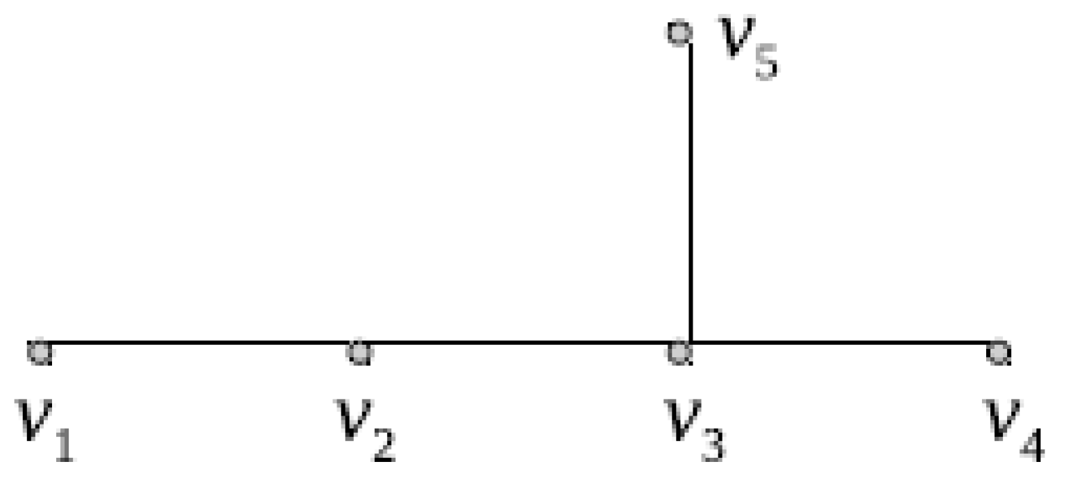
By a chemical tree, we mean a tree which has all vertices of degree less than or equal to 4.

Example 3.

In Figure 1, we depicted a chemical tree of order $n=5$.

The distance matrix of T is

$$D(T)=\left(\begin{array}{ccccc}0& 1& 2& 3& 3\\ 1& 0& 1& 2& 2\\ 2& 1& 0& 1& 1\\ 3& 2& 1& 0& 2\\ 3& 2& 1& 2& 0\end{array}\right).$$

Let ${\mu }_1,\dots ,{\mu }_5$ be the distance eigenvalues of the tree T. Then one can easily see that ${\mu }_1=7.46$, ${\mu }_2=-0.51$, ${\mu }_3=-1.08$, ${\mu }_4=-2$ and ${\mu }_5=-3.86$. Note that, as $D_0(T)=D(T)$, taking $\alpha =0$ in Theorem 8, then for $n=5$ we get $-6\sqrt{\frac{k-1}{6-k}}\le {\mu }_k\le 6\sqrt{\frac{5-k}{k}}$, for any $1\le k\le 5$. For example, $-6\le {\mu }_1\le 12$ and $-3\le {\mu }_2\le 7.3$.

4. Conclusions

Motivated by an article entitled “Merging the A- and Q-spectral theories” by V. Nikiforov [33], recently, Cui et al. [15] dealt with the integration of spectra of distance matrix and distance signless Laplacian through elegant convex combinations accommodating vertex transmissions as well as distance matrix. For $\alpha \in [0,1]$, the generalized distance matrix is known as $D_{\alpha }(G)=\alpha Tr(G)+(1-\alpha )D(G)$. Our results shed light on some properties of $D_{\alpha }(G)$ and contribute to establishing new inequalities (such as lower and upper bounds) connecting varied interesting graph invariants. We established some bounds for the generalized distance spectral radius for a connected graph using various identities like the number of vertices n, the diameter, the minimum degree, the second minimum degree, the transmission degree, the second transmission degree and the parameter $\alpha$, improving some bounds recently given in the literature. We also characterized the extremal graphs attaining these bounds. Notice that the current work mainly focuses to determine some bounds for the spectral radius (largest eigenvalue) of the generalized distance matrix. It would be interesting to derive some bounds for other important eigenvalues such as the smallest eigenvalue as well as the second largest eigenvalue of this matrix.